Bearing Fault Diagnosis with Hybrid CNN-RNN: A Unified-Loop Hyperparameter Optimization Framework via Surrogate-Based Bayesian Optimization

1  Introduction

The transition to Industry 4.0 has underscored the strategic importance of PHM in various industries [1]. In particular, rolling element bearings are critical components of rotating machinery, which serve as the core power source for modern manufacturing and power generation facilities [2]. Bearing failures account for 45%–55% of all rotating machinery breakdowns [3–6], leading to unexpected downtime and increased maintenance costs [7,8]. Therefore, the ability to detect bearing anomalies early and diagnose them accurately is a fundamental technology for ensuring system reliability and safety of rotating machinery.

Conventional approaches to bearing fault diagnosis have relied on handcrafted features derived from expert knowledge, typically extracted through signal processing techniques such as envelope analysis and frequency band selection [9]. Early studies employed classical machine learning classifiers, including Support Vector Machines (SVM) and shallow Artificial Neural Networks (ANN), to learn from these engineered features [10]. For instance, Ribeiro et al. [11] proposed a technique to identify rotating machinery faults using similarity-based modeling, and Marins et al. [12] presented an improved model operation procedure to enhance the bearing classification accuracy. However, such approaches depend heavily on expert heuristics, introducing the risk of information loss and systematic bias [13], and tend to generalize poorly under varying operating conditions [14].

These limitations have accelerated the adoption of Deep Learning (DL)-based end-to-end models, which are capable of learning discriminative features directly from raw data. By eliminating the need for manual feature engineering, DL-based methods have fundamentally shifted the diagnostic paradigm [15,16], and hybrid models that simultaneously utilize time and frequency information have shown particularly outstanding performance [17,18]. In addition, recent studies have demonstrated that robust fault identification is possible even under variable conditions using pre-training and transfer learning techniques [19]. More recently, large language model (LLM)-based approaches have begun to be applied to bearing fault diagnosis, ranging from parameter-efficient fine-tuning of pre-trained LLMs on vibration signals [20] to multimodal frameworks that unify vibration signals and textual prompts within a single model [21]. While such foundation-model approaches represent a complementary direction oriented toward cross-domain transfer and representation reuse, the present study focuses on the integrated optimization of physically motivated preprocessing and supervised hybrid CNN–RNN diagnosis, and LLM-based methods are therefore noted here as concurrent research progress rather than direct comparison targets.

Despite these advances, most existing studies still optimize preprocessing, Hyper Parameter Optimization (HPO), and decision fusion as isolated stages [22], leaving three methodological gaps unaddressed. First, the absence of inter-stage coupling limits the global optimality of the overall system, as preprocessing choices, model hyperparameters, and fusion strategies are tuned without explicit awareness of one another. Second, inconsistent management of data splitting, normalization standards, and execution environments across stages undermines research reproducibility. Third, when new datasets or operating conditions are introduced, the absence of a shared optimization context requires costly retuning of the entire pipeline, limiting the practical efficiency of model development. Addressing these three gaps requires a framework with three capabilities: explicit information propagation between stages, consistent execution under shared normalization boundaries and random seeds, and reuse of the same optimization setup across datasets or operating conditions without per-stage reconstruction.

Existing approaches, including end-to-end pipeline optimization, HPO combined with late-stage stacking, prior hybrid time-domain and time-frequency domain bearing diagnostic frameworks [17], and modern AutoML systems, address parts of these requirements. However, they still leave physically motivated preprocessing screening, branch-level HPO, and decision-level fusion only partially coupled.

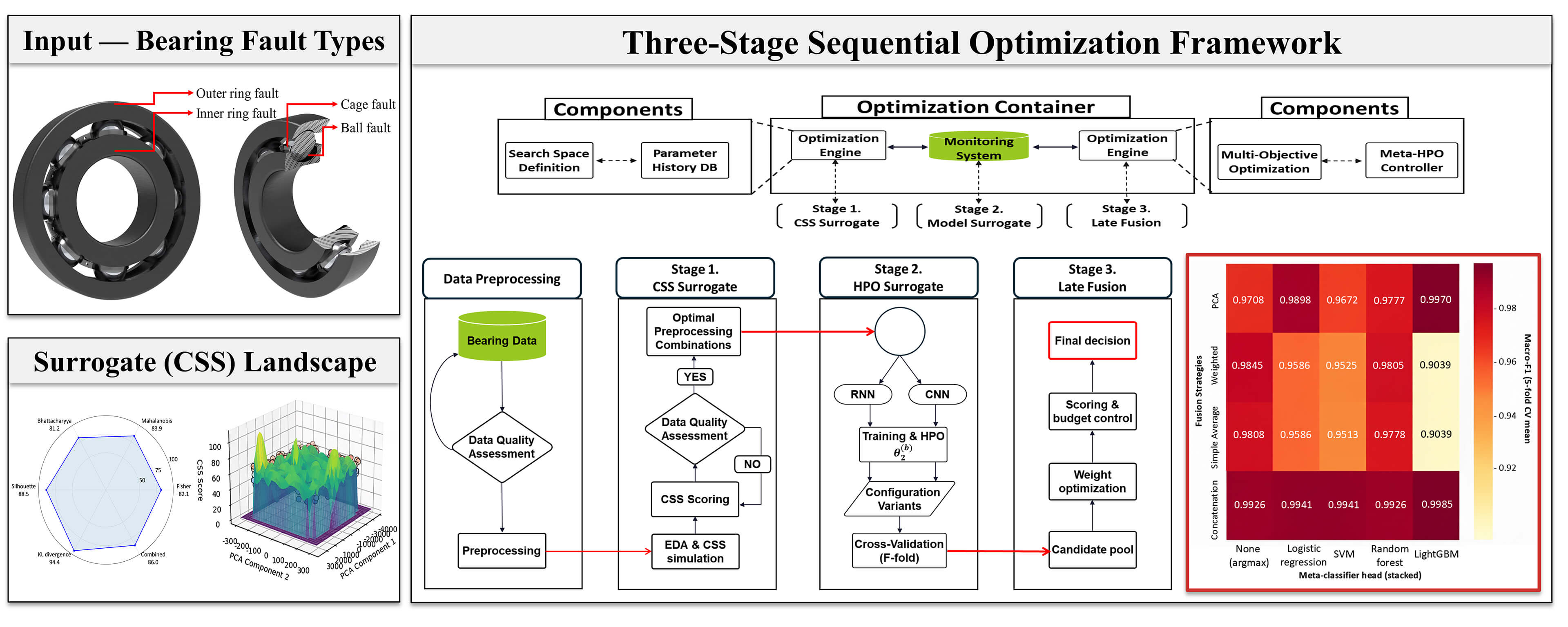
To meet these requirements, this study proposes an integrated global optimization framework encompassing preprocessing, model training, and decision fusion. The proposed ‘Three-Stage Sequential Optimization Framework’ screens preprocessing candidates that reflect the physical characteristics of bearing faults using the CSS metric in a training-free manner (Stage 1), propagates them as optimization inputs for the time/frequency branch models (Stage 2), and integrates the resulting branch outputs into an Out-Of-Fold (OOF)-based weighted late-fusion module (Stage 3), thereby restoring the inter-stage coupling missing in conventional pipelines. All these processes were consistently performed on a single optimization container composed of LHS [23]–KRG(EI) [24]–BOHB [25], under shared normalization boundaries and fixed random seeds, so that the same container can be reused across datasets and operating conditions without per-stage reconstruction. This unified execution simultaneously secures research reproducibility and reduces the retuning cost incurred by fragmented pipelines.

To validate the proposed framework, a two-step experimental approach was adopted. First, a sanity check was conducted on the CWRU [26] dataset to verify that the integrated optimization of preprocessing, model training, and fusion operated correctly with cohesive inter-stage outputs. Second, the primary evaluation was performed on the MAFAULDA [27] dataset to assess generalization across diverse operational conditions, including speed, load, and noise. Detailed quantitative results are presented in the confusion matrices, the fusion heatmap, and the stability box plot in Sections 3.3 and 4.

The primary contributions of this study are as follows: First, the three diagnostic stages—preprocessing screening, dual-branch HPO, and decision fusion—are integrated within a single surrogate-based optimization container; the contribution lies not in the individual components but in the way they are orchestrated: LHS [23] distributes the initial exploration points evenly across the design space, KRG(EI) [24] guides the exploration through a surrogate model, and BOHB [25] allocates computational budget across multiple fidelity levels so that inferior candidates are eliminated early, and this three-stage search structure operates identically across all three diagnostic stages. This structure is operated under shared normalization boundaries and fixed random seeds, directly addressing the inter-stage decoupling, reproducibility, and retuning-cost gaps identified above. Second, the training-free CSS metric brings preprocessing selection—conventionally treated as a pre-hoc step—into the optimization loop itself. Specifically, preprocessing candidates are constructed to reflect the characteristic fault frequencies of outer race, inner race, rolling element, and cage defects, and are screened by CSS without model training, substantially reducing the exploration cost in Stage 1. Third, the out-of-fold posteriors collected from the top-K configurations obtained by Stage 2 HPO in each branch are passed as inputs to a stacking meta-classifier in Stage 3, so that the complementary information of the heterogeneous time-frequency CNN and time-domain GRU branches is exploited at the decision level without additional model training costs.

The remainder of this paper is organized as follows. Section 2 describes the main methodological components of the proposed framework, including bearing fault characteristics, training-free CSS, hybrid branch models, and decision fusion. Section 3, “Proposed Three-Stage Sequential Optimization Framework”, presents the optimization formulation and sequential procedure of the integrated container and includes framework verification on the CWRU dataset. Section 4 reports the main performance evaluation results on the MAFAULDA dataset, including a comparative analysis and stability assessment. Finally, Section 5 concludes this paper.

2  Proposed Methodology

This section presents the core methodological components of the proposed framework, which systematically combines physical domain knowledge with data-driven evaluation metrics. Section 2.1 describes the physical basis of the bearing fault signals and introduces the Class Separability Score (CSS) for training-free preprocessing evaluation. Section 2.2 describes the hybrid model architecture comprising the time-domain and time–frequency-domain branches. Section 2.3 presents the decision-level fusion strategy, and Section 2.4 describes the unified optimization container. The three stages are not optimized simultaneously; rather, they are processed sequentially within the container, while Latin Hypercube Sampling (LHS), Kriging with Expected Improvement (EI), and BOHB are coordinated under a shared execution environment.

2.1 Problem Definition and Bearing Priors

Structural defects in bearings occur as localized damage to the outer race, inner race, ball, or cage (Fig. 1). Each time a rolling element traverses a defect site, a repetitive impulse is generated that excites the structural resonances and produces Amplitude-Modulated (AM) vibration responses [9,26]. Consequently, distinct periodic components and modulation patterns emerge in the time and time–frequency domains for each defect type. Therefore, preserving and accentuating these physical signatures through appropriate preprocessing is a critical determinant of diagnostic performance.

Figure 1: Schematic of bearing structural components and characteristic fault frequencies (BPFO, BPFI, BSF, and FTF).

Bearing fault components manifest as characteristic—Ball Pass Frequency of the Outer race (BPFO), Ball Pass Frequency of the Inner race (BPFI), Ball Spin Frequency (BSF), and Fundamental Train Frequency (FTF)—determined by the shaft rotational frequency and the bearing’s geometric structure, as well as their sidebands (Fig. 1). The present study incorporates these physical priors into the preprocessing design space by parameterizing the center frequency and bandwidth of bandpass filters such that fault-related frequency bands are reliably isolated in the time–frequency representation. Robust scaling was further applied to mitigate the spectral distortion arising from energy-scale differences across frequency intervals. Once the preprocessing parameters and normalization boundaries were determined, they were frozen for all subsequent stages, ensuring a consistent input format across model optimization and decision-level fusion. Despite this design, in real-world operating environments—particularly those involving variable speeds—temporal drift and asymmetric sideband spreading cause the effectiveness of fixed-band preprocessing to vary across conditions, thereby altering the inter-class separation and covariance structure of the feature space. Therefore, it is essential to establish a systematic procedure for comparing and selecting optimal preprocessing candidates. Because the preprocessing design space, which includes the band center, bandwidth, normalization method, and other parameters, is combinatorially large, validation through deep learning training is computationally prohibitive.

Accordingly, Stage 1 performs training-free screening by quantifying the class separability induced by each preprocessing candidate θ1, independently for each branch θ1,RNN and θ1,CNN. Here, θ1 denotes a candidate set of preprocessing parameters, such as filter cutoff frequencies, center frequency, bandwidth, and normalization settings, and is optimized independently for the RNN and CNN branches. To avoid confusing this screening step with the final model input, the preprocessed segments are represented only by lightweight proxy descriptors composed of seven amplitude- and distribution-related statistics: mean, standard deviation, kurtosis, skewness, peak value, peak-to-peak value, and root mean square (RMS). These descriptors are not used as the final inputs to the CNN or GRU models; rather, they summarize candidate-induced changes in signal energy, impulsiveness, dispersion, and distributional asymmetry, enabling the diagnostic relevance of each preprocessing candidate to be evaluated at low computational cost. The CSS is then computed over all available segments of the target dataset, without balanced sub-sampling or condition-wise reweighting, and is used to rank preprocessing candidates according to their class-separation capability under the naturally observed operating-condition distribution. Consequently, the original class proportions and the full range of operating conditions are preserved; the number of segments may differ across classes, and the resulting CSS represents condition-aggregated separability over the full dataset rather than separability optimized for a specific operating regime. Specifically, normalized scores zk,t are computed using five metrics—Mahalanobis Distance (DM), Kullback–Leibler Divergence (DKL), Silhouette Score (Ss), Bhattacharyya Distance (DB), and Fisher’s Discriminant Ratio (RF) (see Appendix A for detailed definitions)—and are linearly aggregated with equal weights (wk=0.2) to define the final CSS as follows:

CSSt= ∑k=15wkzk,t(1)

here, wk denotes the equal weight assigned to each of the five metrics and zk,t represents the normalized score of the k-th metric evaluated on the feature space induced by preprocessing candidate θ1,m, and ∀m∈{RNN,CNN}. In this study, equal weights are assigned to the five metrics, wk = 0.2, to keep the Stage-1 screening criterion simple and training free. Adaptive or non-uniform metric weighting may further improve dataset or branch specific separability assessment, but it would require an additional optimization layer and is therefore left for future work.

The preprocessing search is conducted independently for the RNN and CNN branches because each branch uses a different input representation. The RNN branch operates on time-domain signals, whereas the CNN branch uses time-frequency representations. Accordingly, each branch has its own Stage 1 preprocessing variable θ1,m, and the optimal branch-specific preprocessing candidate is selected by maximizing the corresponding CSS:

θ1,m∗=argmaxθ1,mCSSm(θ1,m)(2)

here, θ1,m denote the branch-specific preprocessing search spaces spanning band center, bandwidth, and normalization parameters. The resulting θ1,m∗ are then frozen as the input specifications for Stage 2. By fixing the preprocessing before model training, the framework eliminates a major source of combinatorial complexity and ensures that all subsequent optimizations operate on a stable, physically grounded feature space.

2.2 Architecture of the Hybrid Diagnostic Model

Because bearing fault signals simultaneously contain impulse signatures in the time domain and modulation patterns in the frequency and time–frequency domains [9,26], single-domain representations are insufficient to capture the entire range of fault-related information. Accordingly, this study proposes a hybrid architecture comprising an RNN branch for time-domain inputs and a CNN branch for time–frequency inputs, enabling the dedicated learning of complementary domain-specific features. In this study, the RNN branch is implemented using a GRU (Section 2.2.1) and the CNN branch using EfficientNetV2 (Section 2.2.2).

Following the sequential optimization strategy of this framework, the optimal preprocessing parameters determined in Stage 1, θ1,RNN∗ and θ1,CNN∗ are applied in a fixed (frozen) manner during the input-generation step of each branch. In Stage 2, the branch-specific model hyperparameters θ2,m are optimized to retain the top-K high-performing model configurations. The OOF posterior probabilities produced by each candidate model during cross-validation are then used as key inputs for the decision-level fusion described in Section 2.3.

2.2.1 GRU Branch for Temporal-Domain Impulse Signatures

The GRU branch models the temporal dependencies of defect-induced impulses and the resulting transient decay patterns [9,28]. As illustrated in Fig. 2, a raw vibration segment is converted into a standardized six-axis time-series input through the fixed preprocessing specification θ1,RNN∗ determined in Stage 1. Defining the input for sample n as xn,RNN∈RT×ch, where T denotes the number of time steps and ch denotes the total number of sensor measurement channel. The preprocessed input takes the following form:

xn,RNN=gRNN(sn;θ1,RNN∗)(3)

here, sn denotes the raw signal segment for sample n, gRNN denotes the deterministic preprocessing operator comprising segmentation, filtering, and robust scaling. The resulting sequence is processed by a multi-layer GRU stack [28], and a class-posterior probability vector is produced based on the final hidden state hT:

pn,RNN=softmax(fRNN(xn,RNN;θ2,RNN)),pn,RNN∈ΔC−1(4)

here, fRNN denotes the mapping function comprising the GRU backbone and a fully connected classification head, and ΔC−1 represents the probability simplex over classes. In Stage 2, BOHB-based HPO explores while fixing θ1,RNN∗, using the mean cross-validation performance score FCV (e.g., Macro-F1 score), as the objective:

{θ2,RNN,k∗}k=1K=Top−Kθ2,RNN∈Θ2,RNN(FCV((θ2,RNN|θ1,RNN∗))).(5)

Figure 2: Overview of GRU branch processing time-series input via GRU backbone.

Rather than selecting a single optimum, the Top−K hyperparameter configurations are retained (K=5 in this study) based on the mean cross-validation score. These retained configurations serve as candidate models for Stage 3, where branch-specific posterior outputs are further compared and only the selected branch-wise outputs are used in the final late-fusion step.

Each candidate model MRNN,k generates posteriors for the validation samples in each fold, which are concatenated across all samples to form the OOF posterior matrix:

MRNN,k=MRNN(θ2,RNN,k∗).(6)

2.2.2 EfficientNetV2 Branch for Spatial–Spectral Modulation Patterns

In the frequency domain, bearing faults manifest as complex spectral patterns composed of characteristic frequencies like BPFO and BPFI, their harmonics, and sidebands [9]. The EfficientNetV2 branch is designed to learn both local features and global patterns from time–frequency representations via convolution operations [29]. As shown in Fig. 3, sn is transformed into a Short-Time Fourier Transform (STFT)-based energy map through the fixed preprocessing specification θ1,CNN∗. Spectrograms are concatenated along the channel dimension to form an input tensor xn,CNN∈R224×224×ch:

xn,CNN=gCNN(sn;θ1,CNN∗)(7)

here gCNN denotes the deterministic preprocessing operator that converts the raw signal into STFT-based spectrograms with robust scaling, and the two sensor groups correspond to distinct triaxial measurement channels concatenated along the channel axis. A mapping function fCNN, consisting of the EfficientNetV2 backbone and a classification head, produces the class-posterior probability vector from the input tensor:

pn,CNN=softmax(fCNN(xn,CNN;θ2,CNN)),pn,CNN∈ΔC−1.(8)

Figure 3: Overview of the EfficientNetV2 branch processing of the spectrogram input via the CNN backbone.

The same Stage 2 protocol as the GRU branch is applied to explore the hyperparameter space θ2,CNN. The Top−K model configurations are retained, and the OOF posterior probability matrix for each candidate is stored as:

MCNN,t=MCNN(θ2,CNN,t∗).(9)

The final outputs of Stage 2 are the branch-wise OOF posterior probability sets derived from Eqs. (6) and (9). These cached posteriors are passed to Stage 3 as its sole branch-side inputs (Section 3.2.3).

2.3 Decision-Level Fusion with OOF Posteriors

The Top−K models retained from Stage 2 encode complementary fault signatures across the time and frequency domains. To preserve this complementary information while avoiding the curse of dimensionality inherent in the early fusion of heterogeneous feature spaces, this study adopted late fusion at the posterior level (Fig. 4) [22]. The only inputs at this stage are the OOF posterior sets cached in Stage 2, which provide unbiased training data for deriving generalized combination rules [20]. For each RNN–CNN candidate pair (k, t), the posterior-level late fusion and the corresponding simplex-constrained weight optimization are formulated as follows:

pfused,(k,t)=ωRNN,(k,t)pRNN,k+ωCNN,(k,t)pCNN,t,ωm,(k,t)∗=arg maxωm,(k,t)(FCV(pfused,(k,t)(ωm,(k,t))))(10)

here, pRNN,k and pCNN,t denote the OOF posterior sets produced by the k-th RNN candidate model and the t-th CNN candidate model, respectively. The weight vector ωm,(k,t), consisting of ωRNN,(k,t) and ωCNN,(k,t), determines the relative contributions of the two branch-specific posterior outputs. For each candidate pair (k, t), this weight vector is optimized under nonnegative sum-to-one constraints to maximize the cross-validation objective FCV, which is measured by Macro-F1 in this study.

Figure 4: Schematic of the decision-level fusion. The OOF posteriors from Top−K models are integrated via simplex-constrained weighting.

After obtaining the optimal weight vector for each candidate pair, the final RNN-CNN candidate pair is selected by maximizing the validation performance of the fused OOF posterior as follows:

(k∗,t∗)=arg max(k,t)(FCV(pfused,(k,t)(ωm,(k,t)∗))).(11)

In Stage 3, the fusion weights ω are optimized under the simplex constraint using the same unified optimization container described in Section 2.4, completing the three-stage pipeline.

2.4 Unified Optimization Container

The entire pipeline—preprocessing (Stage 1), model HPO (Stage 2), and decision fusion (Stage 3)—is executed within a single unified optimization container, as illustrated in Fig. 5. Although each stage involves distinct design variables and objective functions, a shared search mechanism ensures consistency and maintainability across the pipeline. Specifically, the container sequentially optimizes the preprocessing parameters θ1,m, the branch-specific model hyperparameters θ2,m, and the fusion weights ω under a unified protocol.

Figure 5: Unified optimization container components utilizing LHS, Kriging, and BOHB protocols.

The container consists of a History DB module, an optimization engine, and a monitoring system. The History DB serves as a shared repository for evaluated configurations and their corresponding outcomes across all stages. The optimization engine is implemented using the following search components:

•   LHS (Latin Hypercube Sampling): which generates an unbiased, space-filling candidate set in the initialization stage [23].

•   Kriging (Gaussian Process) with EI: this approximates the objective landscape from observed data and proposes promising candidates via the Expected Improvement (EI) acquisition function, balancing exploration and exploitation [24,30].

•   BOHB (Bayesian Optimization and Hyperband): which allocates resources in a multi-fidelity manner, performs early stopping for unpromising candidates, and promotes top configurations [25].

Within the proposed unified optimization container, all three stages are processed sequentially under a shared execution environment. The container coordinates Latin Hypercube Sampling (LHS), Kriging with Expected Improvement (EI), and BOHB across the three stages, while maintaining a common search-space definition, evaluation protocol, monitoring system, and parameter history. Importantly, the proposed container does not imply a fully dynamic co-optimization process or an all-at-once global optimization scheme in which all stages are updated simultaneously. Instead, Stage 1 first evaluates preprocessing candidates using the CSS-based separability criterion, the selected preprocessing configuration is then fixed and propagated to Stage 2 for branch-level HPO, and the OOF posterior probabilities obtained from the selected top-K branch models are finally used in Stage 3 for fusion-weight optimization.

The History DB is defined as a shared repository that stores evaluated configurations and their corresponding results across all stages. Specifically, it records preprocessing candidates, CSS scores, selected preprocessing settings, data split indices, normalization boundaries, random seeds, branch-level HPO records, selected top-K model information, OOF posterior probabilities, and fusion weights. Therefore, inter-stage consistency is not achieved through dynamic knowledge transfer between optimizers, but through the reuse of the shared History DB records. This design ensures that the subsequent stages are executed under the same data handling conditions and optimization history, thereby improving reproducibility and maintaining controlled information propagation across the sequential pipeline.

For implementation, the common optimization settings were fixed across all stages. The Kriging surrogate used a Matérn 5/2 kernel as the default covariance function, while an RBF kernel was used when the number of observations was small. A WhiteKernel noise term and response normalization were included to improve numerical stability. In BOHB, the reduction factor was set to η = 3. The search was terminated when the best-so-far objective improved by less than ε=1×10−3 over 5 consecutive trials, unless the predefined per-stage trial budget was reached first. A master random seed was shared across all stages to ensure reproducible candidate generation, data splitting, and optimization behavior.

To accommodate the differing computational costs across stages, the BOHB-controlled resource axis is defined stage-specifically: the number of signal segments for CSS evaluation in Stage 1, the number of training epochs in Stage 2, and the number of cross-validation folds for fusion weight assessment in Stage 3. In Stage 3, the search target is a fusion weight vector rather than a scalar; the container identifies the optimal weight combination under the simplex constraint while improving the evaluation reliability as the fold budget increases.

3  Proposed Three-Stage Sequential Optimization Framework

This section formulates the bearing diagnosis pipeline as a constrained optimization problem and describes its solution under practical computational budget constraints. The key insight is that jointly optimizing all variables is intractable; instead, the problem is decomposed into three sequential sub-problems—preprocessing, model HPO, and fusion—where each stage inherits frozen outputs from its predecessor, progressively narrowing the search space while preserving inter-stage consistency. All stages are executed within the unified optimization container introduced in Section 2.4. Section 2 introduced the individual components, including CSS-guided preprocessing screening, surrogate-based branch HPO, and posterior-level decision fusion. In contrast, this section focuses on how these components are orchestrated into a unified three-stage sequential pipeline, emphasizing inter-stage information flow, stage-wise optimization variables, and budget allocation.

3.1 Optimization Formulation and Sequential Procedure

The performance of the bearing fault diagnosis model is governed by the coupled interactions among preprocessing parameters θ1, model hyperparameters θ2, and decision-fusion weights ω. Since this study selects the top-K models per branch and combines their OOF posteriors via simplex-constrained weighted late fusion, the overall optimization problem is formulated as maximizing the generalization performance FCV over the joint search space of these variables. Here, FCV denotes the average generalization performance (e.g., Macro-F1) estimated by cross-validation on the dataset sn:

θ∗=arg maxθ∈ΩtotalFCV(sn;θ),(12)

here, Ωtotal=ΩRNN×ΩCNN×Ωfused denotes the joint search space under a hypothetical all-at-once (AAO) optimization setting. The branch-specific spaces are defined as ΩRNN=Ω1,RNN×Ω2,RNN and ΩCNN=Ω1,CNN×Ω2,CNN, where Ω1,RNN and Ω1,CNN denote the preprocessing design spaces for the RNN and CNN branches, respectively. In the present implementation, 77 preprocessing candidates were considered for the RNN branch and 26 candidates for the CNN branch, resulting in 103 preprocessing-related candidates in total, including signal segmentation and filtering settings. The spaces Ω2,RNN and Ω2,CNN denote the branch-specific model hyperparameter spaces, including network depth, width, learning rate, batch size, dropout, optimizer, and scheduler. In addition, Ωfused denotes the simplex-constrained fusion-weight space. In principle, an AAO strategy that jointly explores all variables may provide a more globally coordinated solution. However, the combinatorial growth of the joint search space and the need to retrain deep models for each candidate configuration make AAO computationally impractical [31]. Therefore, the proposed framework adopts a sequential decomposition strategy, in which the selected output of each stage is fixed before the next stage begins. Under this strategy, the practical optimization burden is described by an additive stage-wise budget, Btotal=B1,RNN+B2,RNN+B1,CNN+B2,CNN+Bfused, rather than by exhaustive exploration of the full joint search space. Accordingly, the overall problem is decomposed into three sequential sub-problems. To ensure that this decomposition remains valid, compatibility constraints are imposed to prevent information leakage across stages and to align the input/output formats.

•   Stage 2 Constraint: Model optimization is performed on the frozen feature space generated by the confirmed preprocessing θ1,m*(m∈{RNN,CNN}) from Stage 1.

•   Stage 3 Constraint: Decision fusion uses only the OOF posteriors generated in Stage 2 as inputs, and the base model parameters θ2 are not retrained.

Each decomposed stage has an independent objective function and budget axis and is optimized. The overall execution procedure is summarized in Algorithm 1 [19,31].

3.2 Sequential Execution Procedure

This subsection describes the optimization procedure with reference to the flowchart in Fig. 6. The proposed framework consists of three sequential loops—preprocessing (Stage 1), model HPO (Stage 2), and decision fusion (Stage 3)—where each loop explicitly defines its data flow and outputs to maintain pipeline transparency.

Figure 6: Proposed three-stage sequential optimization framework.

3.2.1 Stage 1: Preprocessing Design Loop (Training-Free)

Because preprocessing defines the input representation for all downstream components, it is optimized first. The first loop (Fig. 6, left) determines the optimal preprocessing strategy prior to model training. Candidate preprocessing configurations θ1 are generated by LHS, and their feature-space separability is quantified using the CSS defined in Section 2.1 as the objective function. The optimization container focuses the search on high-CSS regions, whereas BOHB controls the budget by varying the number of signal segments used for CSS evaluation. Because Stage 1 is conducted without training deep learning models, it removes a major computational bottleneck from the overall pipeline. The converged preprocessing parameters θ1,m* are then finalized and passed to the subsequent stage as frozen input specifications.

3.2.2 Stage 2: Branch HPO Loop (Model Surrogate)

With the preprocessing parameters frozen, the central loop (Fig. 6, center) optimizes the architecture and training hyperparameters θ2,m of each branch (RNN and CNN) on the fixed input representations from Stage 1. Candidate configurations are evaluated by Cross-Validation (CV) performance, whereas BOHB treats the number of training epochs as the budget and applies early stopping to terminate underperforming trials. Unlike conventional HPO that returns a single best configuration, Stage 2 retains the top-K validated configurations per branch and caches their OOF posteriors as the only inputs to Stage 3.

3.2.3 Stage 3: Late Fusion Loop (Decision Level)

Following the posterior-level fusion formulation introduced in Section 2.3, Stage 3 optimizes the simplex-constrained fusion weights using the cached OOF posteriors produced by the top-K branch candidates in Stage 2, without retraining the base models. For each RNN–CNN candidate pair (k,t), the fused posterior is computed as a weighted combination of the corresponding RNN and CNN OOF posterior vectors. The fusion weights are constrained to be non-negative and sum to one, and the optimal candidate pair and its corresponding weights are selected by maximizing the cross-validation objective.

The Stage 3 loop follows the same convergence rule defined in Section 3.1, with ε=1×10−3, k = 5, while the predefined budget cap serves as the upper limit when the convergence criterion is not satisfied. In this stage, the budget controls the reliability of the OOF-based fusion evaluation rather than additional base-model training. The selected fusion weights are then applied to the final decision module to combine the complementary outputs of the time-domain RNN and time-frequency CNN branches.

3.2.4 Budget Schedule and Early-Stopping Policy

All three stages define a stage-specific budget axis within the same optimization container and maintain the search efficiency through multi-fidelity promotion and early stopping policies [31]. The key outputs are propagated sequentially to compose the pipeline: Stage 1 yields the branch-wise optimal preprocessing θ1,m*; Stage 2 yields the top-K configurations and the corresponding OOF posterior sets for each branch; and Stage 3 yields the optimal fusion weights ω* satisfying the simplex constraint, completing the overall optimization. The objective function, budget axis, maximum budget, promotion, and stopping criteria for each stage are summarized in Table 1, and the final selection criterion is illustrated as follows:

θ1,RNN∗,θ1,CNN∗⟶Stage 2MRNN(θ2,RNN,k∗),MCNN(θ2,CNN,t∗)⟶Stage 3{ωRNN,(k∗,t∗)∗,ωCNN,(k∗,t∗)∗},pfused.(13)

3.3 Framework Verification on CWRU

This subsection verifies that the proposed framework operates reliably as designed and that the stage-wise interfaces are consistently integrated into the framework. A sanity check was conducted on the CWRU dataset, which is a widely used benchmark for bearing fault diagnosis. The dataset comprises four classes: Normal, Outer, Inner, and Ball faults. To ensure reproducibility, the data split protocol and normalization boundaries were fixed for all experiments in accordance with Sections 2.1 and 3.2.4, respectively. In particular, normalization was applied within each fold using statistics computed exclusively from the corresponding training set, thereby preventing data leakage into the validation data.

3.3.1 Effect of Training-Free Preprocessing Optimization (Stage 1)

In Stage 1, branch-wise preprocessing is optimized independently to improve the quality of the resulting feature space. The radar chart in Fig. 7a summarizes the CSS component scores after applying optimized preprocessing parameters. All indicators—Fisher’s discriminant ratio (82.1), Mahalanobis distance (83.9), Bhattacharyya distance (81.2), silhouette score (88.5), and KL divergence (94.4)—remained consistently high, yielding a combined score of 86.0. These results indicate that the selected preprocessing candidate improved multiple aspects of class separability, including distance-based separation, distributional discrepancy, and local cluster cohesion, rather than relying on a single metric.

Figure 7: (a) CSS radar chart on CWRU after Stage 1; (b) PCA projection of the optimized feature space.

The Principal Component Analysis (PCA) projection in Fig. 7b, which visualizes the high-dimensional feature space on its two leading principal components, further supports this trend. The Global Candidate selected by Stage 1 is located within a broad high-CSS region rather than on an isolated peak, indicating that the chosen preprocessing configuration is robust to local perturbations in the design space. Although the projection provides only a low-dimensional visualization, the observed landscape suggests that the selected preprocessing parameters preserve fault-relevant variations that are useful for subsequent model training. Overall, these results indicate that CSS-based criteria can screen promising preprocessing candidates without model training. The selected parameters are then frozen as the input specifications for Stage 2, establishing a fixed feature space for subsequent branch-specific model optimization.

3.3.2 Stage 2: Branch-Wise HPO Convergence and Top-5 Selection

The Stage 2 HPO process, conducted on the finalized preprocessed inputs, illustrates the efficiency of BOHB. In the optimization trace shown in Fig. 8a, the initial exploration phase (Trials 0–20) evaluates diverse hyperparameter combinations and exhibits large performance variability. As BOHB progressively filters out low-performing candidates and allocates more resources to promising configurations, the later trials show a tendency toward stable high validation performance. Quantitatively, the trace satisfied the convergence criterion introduced in Section 3.1, indicating that the search reached a stable plateau before exhausting the predefined budget. This plateau behavior reflects the budget–performance trade-off inherent in multi-fidelity search: most of the improvement in validation Macro-F1 was achieved during the early-to-mid trials, whereas subsequent evaluations provided only marginal gains. This supports the use of an explicit budget cap together with the convergence criterion to control the search cost.

Figure 8: (a) BOHB optimization trace on CWRU; (b) hyperparameter importance ranking on CWRU.

The parameter-importance analysis in Fig. 8b indicates that the dropout (0.302) and learning rate (0.284) contribute most to validation performance, suggesting that regularization strength and learning dynamics are the dominant factors in Stage 2 model optimization. The remaining hyperparameters show comparatively smaller importance values within the explored ranges, indicating that the selected search region is not dominated by a single secondary hyperparameter. The selected top-K models generate OOF posteriors on the validation data, which are passed to Stage 3. To balance the combinatorial search cost in Stage 3 with the performance stability, K was fixed to 5. These OOF posteriors, together with the frozen preprocessing from Stage 1, formed the complete input for the final fusion stage.

3.3.3 Stage 3: Effect of Late Fusion

In the final stage, decision-level fusion was performed using the OOF posteriors. Fig. 9a–c compares the confusion matrices of the single-branch baselines (Fig. 9a: GRU, Fig. 9b: EfficientNetV2) with the proposed late fusion (Fig. 9c). The GRU baseline shows noticeable cross-confusion between the ball and inner faults, and EfficientNetV2 exhibited a similar tendency. This result suggests that the two single-branch models capture partially overlapping but not identical fault-discriminative information.

Figure 9: (a) confusion matrix of the GRU baseline on CWRU; (b) confusion matrix of the EfficientNetV2 baseline on CWRU; (c) confusion matrix of the proposed late fusion method on CWRU.

In contrast, late fusion substantially reduces these cross-confusions and produces a more concentrated diagonal structure in the confusion matrix. This improvement indicates that combining the time-domain information captured by the GRU branch and the time-frequency information captured by the CNN branch provides complementary decision evidence. Unlike a heuristic average, the fusion weights are optimized using the validation objective, allowing the relative contributions of the two branches to be adjusted according to their OOF posterior performance. Overall, the CWRU validation results show that the proposed decision-level fusion improves the classification consistency over the individual branch models. In Section 4, the framework is further evaluated on the more challenging MAFAULDA dataset.

4  Performance Evaluation and Results

After verifying the pipeline integrity on the CWRU dataset, this section evaluates the diagnostic performance and stability of the proposed framework on the MAFAULDA dataset, which poses more challenging conditions, including variable operating regimes (load and speed variations) and class imbalance. The evaluation proceeds in the following order: definition of the experimental environment and protocol, performance comparison across the fusion strategies, and stability analysis.

4.1 Evaluation Setup

To ensure fairness and reproducibility, all experiments in this section strictly followed the normalization principles and fixed initialization strategies established in Sections 2.1 and 3.2.4. The dataset used was MAFAULDA, with four fault classes identical to those used in the CWRU verification (Normal, Outer Race, Inner Race, and Ball). To account for data spanning various rotational speeds and load conditions, all samples were randomly shuffled, and five-fold cross-validation was performed. To prevent data leakage, normalization parameters were estimated only from the training split in each fold and applied identically to the corresponding validation/test split.

To clearly control variables in comparative experiments, all models keep the outputs from Stages 1–2 fixed (preprocessing parameters and top-K OOF posteriors), and only the decision fusion strategy in Stage 3 is varied to analyze performance differences. Here, top-K refers to the model configurations selected based on Macro-F1 in Stage 2, and in this study is fixed to 5. For evaluation, five-fold cross-validation was repeated three times with different random seeds to compute the mean and standard deviation. The performance metrics include the Macro-F1 score (robust to class imbalance) and accuracy. To verify statistical significance, a Wilcoxon signed-rank test (α=0.05) is performed using paired Macro-F1 scores within the same fold as samples, ensuring the reliability of the results [32].

4.2 Baselines and Comparative Performance

Five fusion rules methods, namely simple average, weighted average, and PCA-based projection, were combined with five meta-classifier heads: none/argmax, logistic regression, SVM, random forest, and LightGBM. Here, the argmax head corresponds to a non-learning fusion baseline, in which the final class is determined by the maximum posterior score without using an additional meta-classifier. Single-branch baselines, including GRU-only and EfficientNetV2-only models obtained from the same Stage 1–2 outputs, were also evaluated for reference. Fig. 10 visualizes the performance distribution across these fusion strategies in the form of a heatmap.

Figure 10: Classifier performance by fusion strategy on MAFAULDA. Best result: Concatenation + LightGBM (Macro-F1 0.9985).

Linear combination rules, such as simple average and weighted average, yielded relatively low performance in some combinations, for example weighted average and LightGBM with a Macro-F1 of 0.9039. This suggests that simple linear mixing may not sufficiently preserve the complementary posterior information produced by the CNN and RNN branches. In contrast, the proposed concatenation-based stacking strategy achieved consistently strong performance across meta-classifiers and obtained the best result when combined with LightGBM, reaching a Macro-F1 of 0.9985. This result indicates that concatenation can be effective because it preserves the branch-specific posterior outputs as an input feature vector for the meta-classifier, allowing the meta-model to learn heterogeneous posterior patterns that may not be captured by simple averaging rules.

However, this performance gain is accompanied by increased computational cost. Concatenation-based stacking requires an additional learning-based meta-classifier and therefore introduces extra training, validation, and model-selection overhead at the fusion stage. Thus, while concatenation and LightGBM provides an upper-performance reference among the evaluated fusion strategies, it is less attractive when computational efficiency and pipeline simplicity are prioritized. In this regard, the simplex-constrained weighted late fusion used in the proposed framework offers a more cost-effective alternative by combining branch-level posterior outputs without introducing a high-complexity meta-classifier.

This combination also showed an improvement over the next-best non-learning baseline, Argmax, which achieved a Macro-F1 of 0.9926, with a performance gap of Δ=0.0059. Overall, these results suggest that learning-based fusion can improve classification performance by exploiting complementary posterior information from the CNN and RNN branches, whereas non-learning fusion rules provide a simpler but less flexible decision mechanism.

4.3 Stability Analysis

The reliability of a diagnostic system depends not only on its accuracy but also on its stability across data variation. Here, stability is quantified as the standard deviation of the Macro-F1 across five-fold cross-validation folds. Fig. 11 presents the distribution of the cross-validation standard deviation (Macro-F1) for each fusion strategy using a box plot. Among the strategies evaluated, the concatenation strategy achieved the lowest standard deviation (median ≈ 0.008), demonstrating the strongest stability. This suggests that directly passing concatenated OOF posteriors from the top-5 models of each branch to LightGBM preserves the discriminative information and yields more robust convergence under local data noise and split-induced variation. Overall, the proposed framework achieves both the highest diagnostic accuracy (Macro-F1 = 0.9985) and the strongest reproducibility by combining concatenation-based stacking with LightGBM under five-fold cross-validation.

Figure 11: Performance stability by fusion method (CV standard deviation of Macro-F1).

5  Conclusion

This study proposed a three-stage sequential optimization framework that unifies preprocessing, model optimization, and decision fusion into a single coherent workflow, addressing the persistent fragmentation in bearing fault diagnosis pipelines. The framework reduced the early exploration cost by screening preprocessing candidates using the training-free CSS index, which reflects the physical characteristics of bearing faults. Within the resulting fixed feature space, it then performed efficient hyperparameter optimization for the time- and time–frequency-branch models and finalized decisions via late-fusion weight optimization using the OOF posteriors of the top-K models. Moreover, by adopting multi-fidelity BOHB inside a unified optimization container, the framework explicitly controlled the computation budget and mitigated inefficiencies during the search.

Experimental validation on the CWRU and MAFAULDA datasets showed that the proposed framework including the training-free CSS-based preprocessing screening stage, achieved reliable diagnostic performance under controlled benchmark conditions, suggesting its practical promise for laboratory-scale diagnostics, test-bench monitoring, and other industrial settings in which sensing conditions are relatively stable and representative fault patterns are sufficiently captured. In particular, the strong performance on MAFAULDA indicates that the proposed stage-wise design can provide highly reproducible fault identification when the signal environment is well structured. These results suggest that the proposed framework can serve as a practical basis for reducing reliance on manual tuning and supporting a more systematic and reproducible diagnostic pipeline under controlled sensing conditions.

These results demonstrate strong potential, while full field readiness requires further validation under deployment-relevant conditions, including non-stationary speed profiles with rapid transients, cross-domain variability across machines and sensing setups, limited availability of real fault samples, and computational constraints in online or edge environments. Future work will address these aspects by incorporating order tracking and cyclostationary analysis for nonstationary operation, domain adaptation to mitigate cross-domain performance loss, and few-shot learning to enable reliable diagnosis with scarce fault data. Deployment-oriented design guidelines will also be developed to enhance reproducibility, robustness, and inference efficiency in practical PHM systems. In addition, extending the framework to transformer-based and other modern deep learning backbones will allow direct comparison with state-of-the-art methods and evaluate the backbone-agnostic generality of the proposed pipeline. Through these targeted extensions, the proposed framework is expected to evolve into a practical diagnostic pipeline that enhances field reliability and supports maintenance decision-making.

Acknowledgement: Not applicable.

Funding Statement: This work was supported by the National Research Foundation of Korea (NRF) grant funded by the Korea government (MSIT) (RS-2025-24535535) and (RS-2025-25415734).

Author Contributions: The authors confirm contribution to the paper as follows: Jaewan Lee: Conceptualization; Methodology; Software; Validation; Formal analysis; Investigation; Data curation; Writing—original draft preparation; Writing—review and editing; Visualization. Seonghwan Park: Software; Validation; Investigation; Data curation; Writing—review and editing. Junghwan Kook: Conceptualization; Methodology; Validation; Resources; Writing—review and editing; Supervision; Project administration. All authors reviewed and approved the final version of the manuscript.

Availability of Data and Materials: The data that support the findings of this study are available from the corresponding author upon reasonable request.

Ethics Approval: Not applicable.

Conflicts of Interest: The authors declare no conflicts of interest.

Appendix A Supplementary Details for CSS (Class Separability Score)

This appendix provides the mathematical definitions of the key metrics that constitute the CSS proposed in Section 2.1 of the main text, along with the rationale for their academic adoption. To quantitatively assess the quality of the feature space without the training process of machine learning models, this study systematically integrates and utilizes the following five complementary metrics.

Appendix A.1 Mahalanobis Distance (DM): The Mahalanobis distance between two classes i and j, with mean vectors μi,μj and a common covariance matrix Σ, is defined as follows [33]:

DM(μi,μj)=(μi−μj)⊤Σ−1(μi−μj)(A1)

DM is robust to data scaling and correlation structure. As preprocessing highlights defective components and stabilizes the covariance structure, its value typically increases. Although effective for evaluating global mean separation, it relies on unimodal and elliptical distribution assumptions; therefore, it is complemented by combining it with the silhouette score or Bhattacharyya distance.

Appendix A.2 Kullback–Leibler Divergence (DKL): The divergence that represents the structural difference between two probability distributions p(x) and q(x) is defined as follows [34]:

DKL(p|q)=∑x∈Xp(x)ln⁡(p(x)q(x))(A2)

DKL captures high-dimensional differences in distributional shape—such as asymmetry, tail behavior, and multimodality—beyond mean and variance. Because it has a wide dynamic range and is sensitive to density estimation, this study ensured stability via an ln(1+x) prior transformation and robust normalization.

Appendix A.3 Silhouette Score (Ss): The silhouette coefficient s(i) for a data point i is computed using the average intra-cluster distance a(i) and the average distance to the nearest neighboring cluster b(i), as follows [35]:

s(i)=b(i)−a(i)max{a(i),b(i)},S=1N ∑i=1Ns(i)(A3)

It remains valid under nonlinear decision boundaries, and a higher S indicates tighter clustering in the feature space. Unlike global statistical indicators, it focuses on local cluster cohesion and detects subtle contaminations near class boundaries.

Appendix A.4 Bhattacharyya Distance (DB): For two distributions defined by (μ1,Σ1) and (μ2,Σ2), the Bhattacharyya distance is computed as [36], and its commonly used closed-form for Gaussian assumptions is often presented with related divergence treatments [37]:

Σ=12(Σ1+Σ2),DB=18(μ1−μ2)TΣ−1(μ1−μ2)+12ln(detΣdetΣ1detΣ2)(A4)

DB quantifies the degree of overlap between distributions by accounting for both the shift in mean vectors and differences in covariance spread.

Appendix A.5 Fisher’s Discriminant Ratio (RF): Fisher’s ratio represents the ratio of between-class scatter to within-class scatter, and a larger RF implies better separability. Using the between-class scatter matrix SB and within-class scatter matrix SW, it is defined as [38]:

SB= ∑k=1Cnk(μk−μ)(μk−μ)⊤,SW= ∑k=1C ∑x∈Ck(x−μk)(x−μk)⊤,RF=tr(SB)tr(SW)(A5)

By condensing multidimensional information into a single scalar, it is efficient for rapidly screening large candidate pools. It is robust for linear boundaries and, when combined with DKL and Ss in nonlinear settings, provides complementary insights.

Appendix A.6 Summary and Integration Procedure: In summary, DM and RF reflect global mean separation, DB quantifies overlap due to variance differences, DKL captures distributional differences between classes, and Ss represents local cluster quality. Since these indicators have different numerical ranges and unit scales, and because DKL has no fixed upper bound, all distance or divergence based metrics are first log-transformed where applicable using ln⁡(1+x). Subsequently, for each metric, Min–Max normalization is performed over the preprocessing candidate pool so that the normalized score lies in the common [0, 1] range. The normalized metrics are then linearly aggregated to compute the final CSS.

References

1. Lee J, Kao HA, Yang S. Service innovation and smart analytics for industry 4.0 and big data environment. Procedia CIRP. 2014;16(4):3–8. doi:10.1016/j.procir.2014.02.001. [Google Scholar] [CrossRef]

2. Latil D, Ngouna RH, Medjaher K, Lhuisset S. Robust data-driven fault diagnostics for rotating machinery operating under varying working conditions. In: Proceedings of the 2023 9th International Conference on Control, Decision and Information Technologies (CoDIT); 2023 Jul 3–6; Rome, Italy. p. 1912–7. [Google Scholar]

3. Chen X, Yang R, Xue Y, Huang M, Ferrero R, Wang Z. Deep transfer learning for bearing fault diagnosis: a systematic review since 2016. IEEE Trans Instrum Meas. 2023;72(1):3508221. doi:10.1109/TIM.2023.3244237. [Google Scholar] [PubMed] [CrossRef]

4. Sun B, Sheng Z, Song P, Sun H, Wang F, Sun X, et al. State-of-the-art detection and diagnosis methods for rolling bearing defects: a comprehensive review. Appl Sci. 2025;15(2):1001. doi:10.3390/app15021001. [Google Scholar] [CrossRef]

5. Liu Q, Dai Z, Lai H, Chen M, Huang H, Fu J, et al. A noval RUL prediction method for rolling bearing: TcLstmNet-CBAM. Sci Rep. 2025;15(1):14055. doi:10.1038/s41598-025-98845-9. [Google Scholar] [PubMed] [CrossRef]

6. Lei C, Wan H, Yu Y, Miao C, Feng R. Fault diagnosis method of rolling bearing under variable operating conditions based on MFCCNN. Proc Inst Mech Eng Part C J Mech Eng Sci. 2025;239(7):2637–48. doi:10.1177/09544062241303382. [Google Scholar] [CrossRef]

7. Singh J, Azamfar M, Li F, Lee J. A systematic review of machine learning algorithms for prognostics and health management of rolling element bearings: fundamentals, concepts and applications. Meas Sci Technol. 2020;32(1):012001. doi:10.1088/1361-6501/ab8df9. [Google Scholar] [PubMed] [CrossRef]

8. Rigas S, Papachristou M, Sotiropoulos I, Alexandridis G. Explainable fault classification and severity diagnosis in rotating machinery using Kolmogorov–Arnold networks. Entropy. 2025;27(4):403. doi:10.3390/e27040403. [Google Scholar] [PubMed] [CrossRef]

9. Randall RB, Antoni J. Rolling element bearing diagnostics—a tutorial. Mech Syst Signal Process. 2011;25(2):485–520. doi:10.1016/j.ymssp.2010.07.017. [Google Scholar] [CrossRef]

10. Yan X, Jia M. A novel optimized SVM classification algorithm with multi-domain feature and its application to fault diagnosis of rolling bearing. Neurocomputing. 2018;313:47–64. doi:10.1016/j.neucom.2018.05.002. [Google Scholar] [CrossRef]

11. Ribeiro F, Marins MA, Netto SL, Silva E. Rotating machinery fault diagnosis using similarity-based models. In: Proceedings of the XXXV Simpósio Brasileiro de Telecomunicações e Processamento de Sinais (SBrT 2017); 2017 Sep 3–6; São Pedro, Brazil. [Google Scholar]

12. Marins MA, Ribeiro FML, Netto SL, da Silva EAB. Improved similarity-based modeling for the classification of rotating-machine failures. J Frankl Inst. 2018;355(4):1913–30. doi:10.1016/j.jfranklin.2017.07.038. [Google Scholar] [CrossRef]

13. Peng J, Kimmig A, Wang D, Niu Z, Fan Z, Wang J, et al. A systematic review of data-driven approaches to fault diagnosis and early warning. J Intell Manuf. 2023;34(8):3277–304. doi:10.1007/s10845-022-02020-0. [Google Scholar] [CrossRef]

14. Zhang Q, Zhao Z, Zhang X, Liu Y, Sun C, Li M, et al. Conditional adversarial domain generalization with a single discriminator for bearing fault diagnosis. IEEE Trans Instrum Meas. 2021;70:3514515. doi:10.1109/TIM.2021.3071350. [Google Scholar] [PubMed] [CrossRef]

15. Zhao R, Yan R, Chen Z, Mao K, Wang P, Gao RX. Deep learning and its applications to machine health monitoring. Mech Syst Signal Process. 2019;115(1):213–37. doi:10.1016/j.ymssp.2018.05.050. [Google Scholar] [CrossRef]

16. Lei Y, Yang B, Jiang X, Jia F, Li N, Nandi AK. Applications of machine learning to machine fault diagnosis: a review and roadmap. Mech Syst Signal Process. 2020;138:106587. doi:10.1016/j.ymssp.2019.106587. [Google Scholar] [CrossRef]

17. Han K, Wang W, Guo J. Research on a bearing fault diagnosis method based on a CNN-LSTM-GRU model. Machines. 2024;12(12):927. doi:10.3390/machines12120927. [Google Scholar] [CrossRef]

18. Shao S, McAleer S, Yan R, Baldi P. Highly accurate machine fault diagnosis using deep transfer learning. IEEE Trans Ind Inform. 2019;15(4):2446–55. doi:10.1109/TII.2018.2864759. [Google Scholar] [PubMed] [CrossRef]

19. Che C, Wang H, Fu Q, Ni X. Deep transfer learning for rolling bearing fault diagnosis under variable operating conditions. Adv Mech Eng. 2019;11(12):1687814019897212. doi:10.1177/1687814019897212. [Google Scholar] [CrossRef]

20. Tao L, Liu H, Ning G, Cao W, Huang B, Lu C. LLM-based framework for bearing fault diagnosis. Mech Syst Signal Process. 2025;224(3):112127. doi:10.1016/j.ymssp.2024.112127. [Google Scholar] [CrossRef]

21. Peng H, Liu J, Du J, Gao J, Wang W. BearLLM: a prior knowledge-enhanced bearing health management framework with unified vibration signal representation. Proc AAAI Conf Artif Intell. 2025;39(19):19866–74. doi:10.1609/aaai.v39i19.34188. [Google Scholar] [CrossRef]

22. Mohandes M, Deriche M, Aliyu SO. Classifiers combination techniques: a comprehensive review. IEEE Access. 2018;6:19626–39. doi:10.1109/ACCESS.2018.2813079. [Google Scholar] [PubMed] [CrossRef]

23. McKay MD, Beckman RJ, Conover WJ. A comparison of three methods for selecting values of input variables in the analysis of output from a computer code. Technometrics. 2000;42(1):55–61. doi:10.1080/00401706.2000.10485979. [Google Scholar] [CrossRef]

24. Martin JD, Simpson TW. Use of Kriging models to approximate deterministic computer models. AIAA J. 2005;43(4):853–63. doi:10.2514/1.8650. [Google Scholar] [CrossRef]

25. Falkner S, Klein A, Hutter F. BOHB: robust and efficient hyperparameter optimization at scale. arXiv:1807.01774. 2018. [Google Scholar]

26. Case Western Reserve University. Bearing data center: seeded fault test data [Internet]. Cleveland, OH, USA: Case School of Engineering; 1997[cited 2024 Nov 4]. Available from: https://engineering.case.edu/bearingdatacenter. [Google Scholar]

27. Signals, Multimedia and Telecommunications Laboratory (SMTCOPPE/Poli/UFRJ. MAFAULDA: machinery fault database [Internet]. Rio de Janeiro, Brazil: Federal University of Rio de Janeiro (UFRJ); [cited 2024 Nov 4]. Available from: http://www02.smt.ufrj.br/~offshore/mfs/page_01.html. [Google Scholar]

28. Chung J, Gulcehre C, Cho K, Bengio Y. Empirical evaluation of gated recurrent neural networks on sequence modeling. arXiv:1412.3555. 2014. [Google Scholar]

29. Tan M, Le QV. EfficientNetV2: smaller models and faster training. In: Proceedings of the 38th International Conference on Machine Learning; 2021 Jul 18–24; Virtual. [Google Scholar]

30. Jones DR, Schonlau M, Welch WJ. Efficient global optimization of expensive black-box functions. J Glob Optim. 1998;13(4):455–92. doi:10.1023/A:1008306431147. [Google Scholar] [CrossRef]

31. Martins JRRA, Lambe AB. Multidisciplinary design optimization: a survey of architectures. AIAA J. 2013;51(9):2049–75. doi:10.2514/1.J051895. [Google Scholar] [CrossRef]

32. Wilcoxon F. Probability tables for individual comparisons by ranking methods. Biometrics. 1947;3(3):119–22. doi:10.2307/3001946. [Google Scholar] [CrossRef]

33. Xiang S, Nie F, Zhang C. Learning a Mahalanobis distance metric for data clustering and classification. Pattern Recognit. 2008;41(12):3600–12. doi:10.1016/j.patcog.2008.05.018. [Google Scholar] [CrossRef]

34. Kullback S, Leibler RA. On information and sufficiency. Ann Math Stat. 1951;22(1):79–86. doi:10.1214/aoms/1177729694. [Google Scholar] [CrossRef]

35. Rousseeuw PJ. Silhouettes: a graphical aid to the interpretation and validation of cluster analysis. J Comput Appl Math. 1987;20:53–65. doi:10.1016/0377-0427(87)90125-7. [Google Scholar] [CrossRef]

36. Bhattacharyya A. On a measure of divergence between two statistical populations defined by their probability distribution. Bull Calcutta Math Soc. 1943;35:99–110. [Google Scholar]

37. Kailath T. The divergence and bhattacharyya distance measures in signal selection. IEEE Trans Commun Technol. 1967;15(1):52–60. doi:10.1109/TCOM.1967.1089532. [Google Scholar] [PubMed] [CrossRef]

38. Fisher RA. The use of multiple measurements in taxonomic problems. Ann Eugen. 1936;7(2):179–88. doi:10.1111/j.1469-1809.1936.tb02137.x. [Google Scholar] [CrossRef]