Physics-Informed Machine Learning Framework for Sulphide Mineralization Mapping in Maitengwe Greenstone Belt Northeastern Botswana

1  Introduction

Greenstone belts are economically significant repositories of mineral deposits and commonly host copper, nickel, iron, manganese, chromite, and gold mineralization [1–4]. The Maitengwe greenstone belt forms part of the Francistown granite–greenstone complex on the Zimbabwe craton [5]. Together with the Matsitama, Tati, and Vumba belts, it belongs to the northeastern Botswana exposure of this cratonic terrane [6]. In the adjacent belts of the Zimbabwe craton, economically important gold, nickel, and copper deposits are commonly associated with sulphides and are frequently localized within shear zones and fault-controlled structures. Examples include the Tekwane, Selkirk, and Phoenix Cu/Ni deposits, as well as the Map Nora, Gold Eagle, Signal Hill, and Mupane gold deposits in the Tati belt [7,8]. Comparable structurally controlled mineralization has also been reported in the Vumba belt and in several nickel sulphide deposits in Zimbabwe, including Damba, Hunters Bay, Trojan, and Shangani [9]. Geological evidence of these adjacent terranes suggests that structurally controlled sulphide deposits might be present, even though no large economic sulphide deposits have been found in the Maitengwe belt. Recent studies have successfully applied machine learning algorithms, particularly random forest, for mineral prospectivity mapping in greenstone belts, comparing fertile and less fertile terrains to identify key geological and structural controls on metal endowment [10].

Geophysical exploration offers an efficient way to study potential sulphide mineralization in greenstone belts where outcrops are scarce and sulphide mineralization is structurally controlled. Aeromagnetic surveys help map lithological boundaries, dykes, folds, faults and shear zones, while induced polarization-electrical resistivity imaging (IP-ERI) surveys complement this data by providing information on chargeability and resistivity anomalies related to sulphides, alteration and lithology. However, traditional advances to inversion (interpretation) are tormented by non-uniqueness, smoothing and noise, especially in complex terrain. This makes it difficult to make the transition from big geophysical anomalies to mineralization plans.

Advances in the field of machine learning have been shown to improve geophysical interpretation, particularly lithological mapping from magnetic, anomaly detection from electrical and electromagnetic data, respectively [11,12]. However, most of the current studies are based on data-driven models, single geophysical data sets, or synthetic benchmarks which are not representative of the geological complexity of the actual exploration scenario [13–15]. Advanced machine learning techniques, including contrastive representation learning and dimensionality reduction, have recently been shown to enhance mineral prospectivity mapping by effectively handling high-dimensional geospatial data and addressing class imbalance challenges [16]. In addition, most such approaches treat geophysical observations as abstract predictors without explicitly constraining the learning process using the spatial behaviour of the underlying physical-property fields.

Physics-informed machine learning offers a more structured alternative by embedding domain knowledge within the model architecture or objective function [17]. In geophysical applications, this can improve stability, support geologically plausible predictions, and reduce the dependence on purely empirical correlations. However, existing physics-informed ML studies in geosciences have focused mainly on forward modelling, seismic inversion, or hydrological systems, with limited application to integrated aeromagnetic and IP–ERI datasets for sulphide exploration. Applications to disseminated sulphide systems in African greenstone belts remain particularly limited. In Fig. 1, location map of the study area showing the Maitengwe Greenstone Belt within the Francistown granite–greenstone complex, northeastern Botswana.

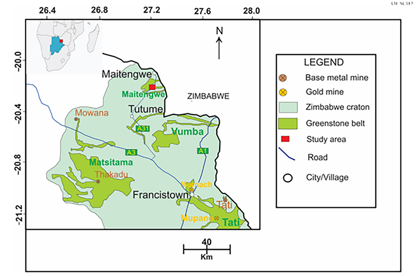
Figure 1: Location of the study area and the regional geology modified from [18], showing the greenstone belts of the Francistown granite–greenstone complex on the southwestern part of the Zimbabwe craton extending into Botswana. Various base-metal and gold mines occur within the Tati and Matsitama greenstone belts.

This study addresses this gap through GeoPhysML, a physics-informed machine-learning framework for sulphide mineralization mapping in the Maitengwe Greenstone Belt, northeastern Botswana. The workflow integrates four main stages: (1) inversion of aeromagnetic and IP–ERI data to establish the structural and physical-property framework; (2) construction of collocated magnetic and electrical features; (3) supervised prediction of mineralization likelihood using a feed-forward neural network with auxiliary resistivity and chargeability outputs constrained by Laplacian smoothness and gradient-based regularization; and (4) uncertainty estimation and geological validation using borehole MTW4. The objective is not to supplant geophysical inversion, but to enhance inversion-based interpretation with the use of physical-property fields, structural attributes, and borehole control in the context of a probabilistic mineralization mapping.

1.1 Geophysical Techniques and Methods

This learning used aeromagnetic and IP-ERI data to determine if the interpreted sulphide mineralization in the Maitengwe Greenstone Belt is structurally controlled. In the detection stage, lithological contacts, magnetic lineaments and structurally potential target zone were identified based on aeromagnetic data. The electrical response of resistivity and chargeability associated with modification and sulphides was described using the ground-based geophysical method of IP-ERI. These methods combine regional scale structural information and local scale electrical property information to aid in geological interpretation and uncertainty in target recognition.

Conventional and enhanced aeromagnetic data were used to map structures and other weak magnetic information that may be significant for mineralization. This increases resolution of subtle anomalies, accentuates structural features, and aids in the interpretation of faults, shear zones, dykes and lithological boundaries. Aeromagnetic data play an important role in mineral exploration and mapping subsurface structures. The use of magnetic data in detecting basement tectonics was demonstrated by Abu El-Ata et al. in Eastern Yemen [19]. Al-Ibiari et al. [20] employed aeromagnetic data for Wadi Zeidun region in Egypt, emphasizing the potential of magnetic techniques in mapping contacts and discontinuities. The authors, Anand and Rajaram [21] were successful in using aeromagnetic data to locate hidden deposits of uranium in the Singhbhum province, in India, for mineral exploration targeting purposes. Leseane et al. [22] used regional aeromagnetic data to develop an aeromagnetic model for structural overprinting criteria in the Hill End Trough, East Gondwana. Robertson et al. [23] interpreted aeromagnetic data in the Franklin area, northern New Zealand, for the purposes of mapping structural features. Rodríguez et al. [24] analysed the Sabinas Basin geotectonic regime using aeromagnetic data and GIS. Basement structures in the northwestern offshore, Abu Dhabi were mapped by Salem and Ali [25] from high-resolution aeromagnetic data. Together these studies clearly show the ability of the aeromagnetic technique to provide useful information to aid in understanding subsurface structural frameworks for mineral exploration.

The IP-ERI method was adopted because, while resistivity might not be sufficient to map the presence of disseminated sulphides, induced polarization will be sensitive to charge storage effects from metallic mineralization. Revil et al. [26] showed this effect clearly, and illustrated how induced polarization was better able to detect the location of pyrite mineralization than electrical conductivity. This is because conductivity is highly sensitive to the amount and connectivity of conductive minerals in the host rock [27]. Thus, in this study, IP–ERI was used to map subsurface resistivity and chargeability to interpret the anomaly zones in terms of the lithological, alteration and structural environment [28].

Inverted IP–ERI responses were analysed as pseudo-2D profiles and as a pseudo-3D stack of parallel profiles. Pseudo-2D sections are useful to detect vertical and horizontal anomalies along individual profiles but they are less effective to infer off-line and 3D features [29]. To overcome this limitation, a pseudo-3D reconstruction was used to enhance the interpretation of anomaly shapes and relationships between profiles. Even so, geophysical interpretation remains affected by non-uniqueness, particularly in potential-field and inversion problems [30]. To reduce this ambiguity, the geophysical results were interpreted jointly with prior geological knowledge, historical geochemical and geophysical information, and borehole constraints from the study area.

1.2 Geological Setting

The Maitengwe greenstone belt is located in the north-eastern part of Botswana. The study area lies south of Maitengwe Village, close to the main tarred road to the village, at approximately 20.00025∘ S and 27.20348∘ E. The terrain is relatively flat and characterized by limited surface exposure.

The Maitengwe greenstone belt forms part of the Francistown granite–greenstone complex situated on the southwestern margin of the Zimbabwe craton, which extends into Botswana. Archaean granitoids and gneissic rocks, together with the greenstone sequences, constitute the crystalline basement. The supracrustal component of the greenstone belt is dominated by mafic and ultramafic metavolcanic rocks. These lithologies have been correlated with the Upper Bulawayan greenstones. The granitoids of the Francistown complex consist mainly of variably foliated tonalite–trondhjemite–granite (TTG) gneisses, with lesser late-kinematic granodiorite, monzonite, and granite [6]. These greenstones have been metamorphosed from low-grade greenschist to amphibolite facies and are strongly deformed and sheared.

Litherlands [31] divided the Maitengwe Group into the lower Maitengwe Banded Iron Formation (BIF), overlain by the Maitengwe Ultramafic Formation. The Maitengwe greenstone belt comprises three main sequences of metasedimentary and metavolcanic rocks, namely the Mpapho banded ironstone formation, the Mazuwe amphibolite, and the Sokwane quartz sericite schist [32]. These lithologies are readily recognized on the aeromagnetic map because of their strong magnetic response. They show relatively limited tectonic disruption, remaining uniformly banded over several hundreds of metres along strike. The ironstones are associated with serpentinite, marble, calci-silicate, iron-free chert, and minor ultramafic schist. Amphibolite becomes more distinctly intercalated with the ironstones toward the upper part of the formation. The Mazuwe Amphibolite unit consists predominantly of amphibolite and ultramafic schist, interbedded with thin ironstone, calcsilicate, serpentinite, and marble/carbonate horizons. The presence of Sokwane quartz sericite schist was confirmed from drillhole information because no outcrop of this unit was observed in the study area [32].

Based on this lithological and structural framework, several geophysical-to-geological associations are expected to constrain the GeoPhysML interpretation:

•   Banded Iron Formation (BIF) and ultramafic rocks → high total magnetic intensity (TMI) and RTP responses

•   Shear zones and faults with dominant NE–SW orientation → strong tilt derivative (TDR) response and linear magnetic anomalies

•   Disseminated sulphides in altered amphibolite → elevated chargeability (mc) with variable resistivity depending on silicification and alteration intensity

•   Quartz–carbonate veins containing sulphides → elevated resistivity and elevated chargeability, corresponding to zones C and III

•   Weathered chloritic amphibolite → low resistivity and low chargeability, corresponding to zones A and I

Drillhole information provides important subsurface constraints for understanding lithological variation and sulphide mineralization in the Maitengwe Greenstone Belt. Borehole data were therefore used to support geophysical interpretation and to validate mineralized zones identified from inversion and machine-learning analysis.

Mineralization is largely hosted in strongly hydrothermally altered amphibolite and ultramafic rocks. It is concentrated within possible shear zones that likely acted as conduits for hydrothermal fluids. Gold values of 0.01–0.65 ppm were reported in hole MTW 1 over the depth interval 110–160 m. The mineralization is disseminated and occurs as blebs, smears, and stringers along carbonate and quartz veins. The available drillholes are shown in Fig. 2.

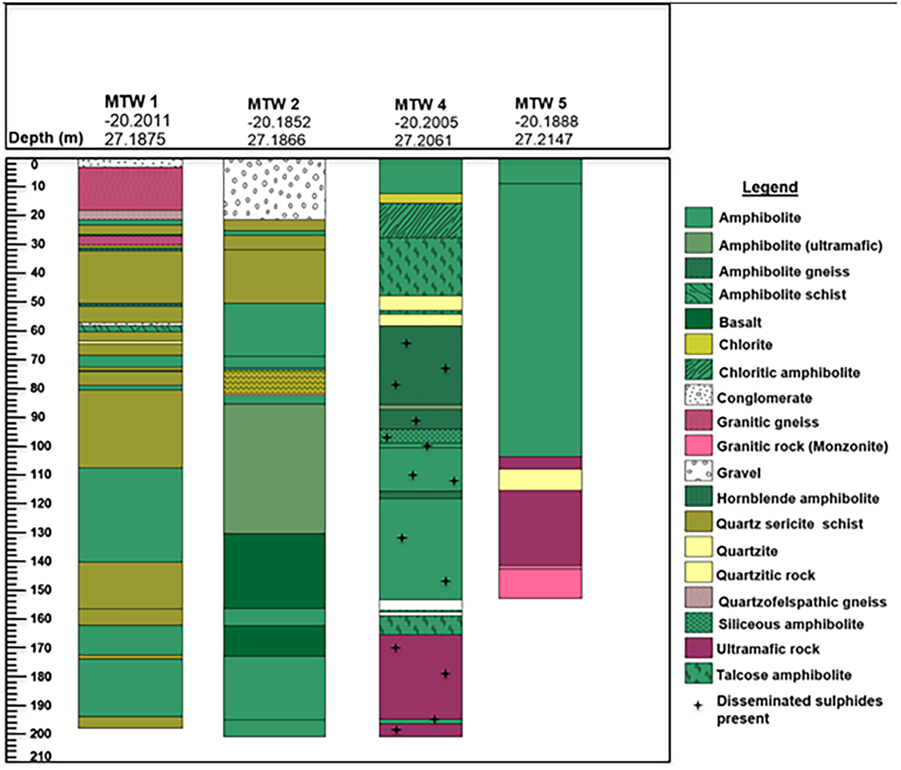
Figure 2: Drill boreholes in the study area showing the stratigraphy of the Maitengwe greenstone belt, modified from [32]. Borehole MTW 4 is closest to the survey area and is therefore used in geological interpretation.

Thin section petrography and X-ray diffraction (XRD) analysis were not available for this study. Sulphide identification is therefore based on borehole logs and geophysical response. This limitation is acknowledged, and future work should include mineralogical characterization.

2  Methodology

The complete workflow comprises four sequential stages. First, aeromagnetic data were processed to extract structural lineaments using total magnetic intensity (TMI), reduced-to-pole (RTP), first vertical derivative (1VD), and tilt derivative ratio (TDR) transformations, while induced polarization–electrical resistivity imaging (IP–ERI) data were inverted to obtain resistivity and chargeability models. Second, all geophysical attributes were co-located onto a common three-dimensional grid with voxel dimensions of 25m×25m×10m. Third, borehole MTW4 provided positive labels corresponding to mineralized intervals and negative labels corresponding to barren intervals, which were assigned to the respective grid cells. Fourth, the GeoPhysML model was trained using 247 labelled cells to predict the probability of mineralization across the entire survey area.

Fig. 3 integrated workflow of the GeoPhysML framework showing data inputs, processing stages, feature fusion, spatial data splitting, model architecture, physics-informed regularization, prediction with uncertainty quantification, and independent validation using borehole MTW4.

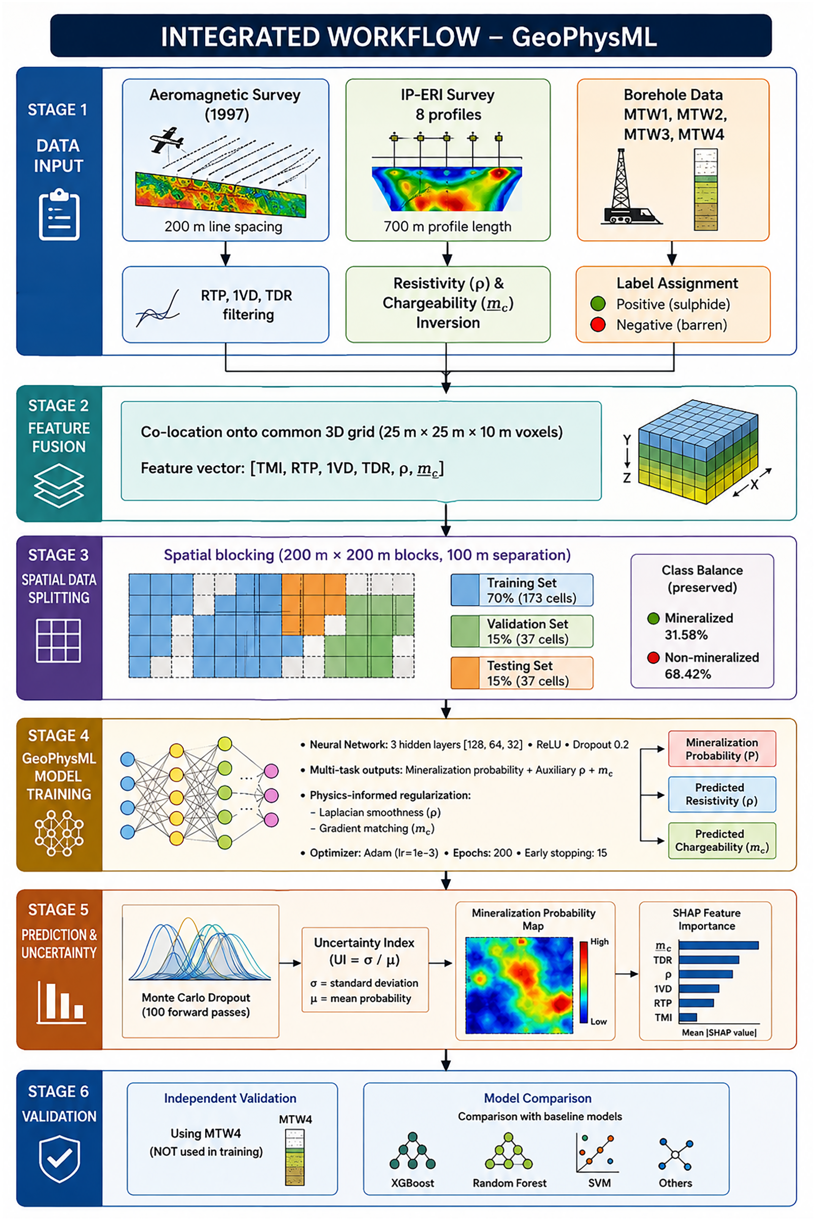
Figure 3: Integrated workflow of the GeoPhysML framework.

2.1 Aeromagnetic Data Processing

The aeromagnetic data used in this study have been provided by the Botswana Geoscience Institute. It is part of the aeromagnetic survey of the Northeast zone, carried out in 1997 by Compagnie Générale Géophysique [33]. The area surveyed was approximately 5520 km2 and the survey consisted of 33,655 km of flight lines flown at a nominal terrain clearance of 80 m. The flight lines had a spacing of 200 m, and the tie lines were flown at an azimuth of 215∘ and spaced at 2000 m. The final product was delivered on a 50 m × 50 m grid in the World Geodetic System 1984 (WGS 84) datum.

Aeromagnetic enhancement was conducted to bring out subtle features of the magnetic field and aid in the mapping of lithological contacts, dykes, shear zones and other important structural features. Recent advances in unsupervised machine learning have provided new approaches for imaging geological structures from aeromagnetic data, complementing traditional derivative-based interpretation methods [34]. The interpretation of the magnetic data used both the intensity and geometric properties of the magnetic response, such as the texture, shape, continuity, orientation, truncation, and offset of anomalies that might represent structural distortion or cross-cutting. Beginning with the Total Magnetic Intensity (TMI) grid, a series of conventional processing steps were undertaken using Geosoft Oasis Montaj version 9.9.1. These enhancement operations involved reduction to the pole (RTP), first vertical derivative (1VD) and tilt derivative (TDR) filtering. These were combined to enhance anomaly edges, to reduce the effect of geomagnetic field-induced positional offset, and to enhance the delineation of lineaments of interest for mineral exploration targeting. These magnetic attributes were also used in the set of features that were incorporated into the GeoPhysML structure.

2.1.1 Geological Interpretation of Magnetic Lineaments

The N–S and subordinate E–W lineaments may represent secondary fracture systems that locally enhanced rock permeability and facilitated fluid migration. Consequently, the intersection zones between the NE–SW and N–S lineaments are interpreted as the most prospective targets for structurally controlled sulphide mineralization, owing to their enhanced potential for fluid focusing, mineral deposition, and ore accumulation.

2.2 Magnetic Data Processing and Interpretation

Magnetic processing was performed to amplify anomaly patterns relevant to the study of structural features and to obtain attributes that are more sensitive to the presence of lithological boundaries, dykes, shear zones and fault-controlled discontinuities in the area than the total magnetic intensity (TMI) anomaly field itself. Let T(x,y) represent the gridded magnetic anomaly field over the area of interest, with x and y being the horizontal coordinates of the map plane. This study has adopted the processing sequence of reduction to the pole (RTP), first vertical derivative (1VD), and tilt derivative (TDR). These operators were chosen to progressively enhance anomaly centering, boundary sharpening and the continuity of structures, which are important for geological interpretation and feature extraction.

Reduction to the Magnetic Pole (RTP)

Magnetic anomalies are usually asymmetric when measured away from the geomagnetic poles since the inducing geomagnetic field is inclined instead of vertical. This means that the maximum magnetic response occurs at a distance from the magnetic cause and that the anomaly shape is not only a function of the geometry and magnetization contrast of the body, but also of the inclination and the declination of the ambient field [35,36]. This asymmetry complicates structural interpretation, especially when anomaly maxima must be related to geological contacts or narrow linear bodies.

The RTP transformation reprojects the observed magnetic response to the equivalent anomaly that would be produced if both the inducing field and the magnetization direction were vertical. In the Fourier domain, the RTP operator may be expressed as

T~RTP(kx,ky)=T~(kx,ky)Lp(kx,ky)Lobs(kx,ky),(1)

where T~(kx,ky) is the Fourier transform of the observed magnetic field T(x,y), (kx,ky) are the horizontal wavenumbers, Lobs is the directional response of the observed inducing field, and Lp is the equivalent response for a vertical field at the magnetic pole. The inverse Fourier transform of T~RTP yields the RTP grid TRTP(x,y).

Essentially, RTP moves the magnetic anomaly closer to the source and helps to reduce the skew effect due to inclined magnetization. This greatly facilitates the interpretation of linear features, contacts and truncations. In this study, the RTP was used as the reference magnetic field to enhance the magnetic anomaly using derivatives and interpret lineaments.

First Vertical Derivative (1VD)

In order to enhance shallow magnetic anomalies and reduce regional effects, the RTP grid was processed by the first vertical derivative (1VD). The first vertical derivative is the rate of change of the magnetic field in the vertical direction and as such highlights high-frequency components related to shallow or structurally abrupt features [25].

Let TRTP(x,y) denote the reduced-to-pole magnetic field. The first vertical derivative is defined as

1VD(x,y)=∂TRTP(x,y)∂z,(2)

where z is the vertical coordinate taken positive downward or upward according to the adopted sign convention. In frequency-domain implementation, differentiation with respect to z is equivalent to multiplication by the radial wavenumber k, where

k=kx2+ky2.(3)

Hence, the first vertical derivative in the Fourier domain is written as

1VD~(kx,ky)=kT~RTP(kx,ky),(4)

with the sign depending on the software convention used for the vertical axis. The inverse transform then gives the spatial-domain derivative field [25,37].

The 1VD reduces the regional effects and amplifies the effect of sharp lateral changes in susceptibility. As a result, contacts, dyke-like features and fault-bounded contrasts are more prominent than the RTP grid. Derivative calculations also enhance the noise, so the 1VD product was interpreted in conjunction with the RTP and TDR grids.

Tilt Derivative (TDR)

While the first vertical derivative is suitable for the enhancement of shallow edges, the dynamic range of the first vertical derivative can be dominated by strong anomalies, obscuring weaker but important anomalies. To counter this effect, the tilt derivative was calculated from the RTP grid. The tilt derivative (also known as the local phase) is the ratio of the vertical gradient to the total horizontal gradient and can be used to enhance the continuity of structural features (lineaments) and to equalise the response of large and small anomalies [38,39].

The total horizontal derivative of the RTP field is first defined as

THDR(x,y)=(∂TRTP∂x)2+(∂TRTP∂y)2,(5)

where ∂TRTP/∂x and ∂TRTP/∂y are the horizontal gradients in the easting and northing directions, respectively. The tilt derivative is then given by

TDR(x,y)=tan−1⁡(∂TRTP∂z(∂TRTP∂x)2+(∂TRTP∂y)2).(6)

Thus, Eq. (6) may also be written compactly as

TDR(x,y)=tan−1(1VD(x,y)THDR(x,y)).(7)

By definition, the tilt angle is bounded within

−π2≤TDR(x,y)≤π2.(8)

A key advantage of the tilt derivative is that the zero contour,

TDR(x,y)=0,

Approximately marks the boundaries of magnetic sources or abrupt variations in susceptibility. Typically, positive values are found over the source and negative values outside it. This makes TDR an excellent method for mapping linear contacts and lineaments in a study area, even when anomalies may have different amplitudes [26,40].

Interpretational Role of the Magnetic Derivatives

The three magnetic grids were interpreted together. The RTP grid was used to better position anomalies over their source, and to delineate the overall regional structure. The 1VD grid was used to identify narrow, shallow magnetic sources, such as lithological contacts, dykes and disturbed magnetic fabric. The TDR Grid was used primarily for the detection of lineaments and continuity as this type of grid permits strong and weak features to be displayed on a similar scale.

The joint processing method was especially useful in the Maitengwe Greenstone Belt for the detection of truncations of magnetic units and the identification of curvilinear high-amplitude magnetic bands construed as iron-rich lithologies and linear magnetic discontinuities interpreted as faults, fractures, or shear zones. They were then combined with the IP-ERI output in the GeoPhysML framework for structurally constrained mineralization mapping.

The enhanced map in Fig. 4a was used to produce a lineament map and was complemented by the 1VD and TDR grids, Fig. 4b and Fig. 4c, respectively. The RTP image shows well developed textural variations in the basement, where the magnetic high (55.9 to 112.0 nT) is interpreted as a broad band of banded ironstones and ultramafic rocks, and the magnetic low (−193.9 to −12.8 nT) is interpreted as a broad cover of sedimentary rocks with smooth magnetic texture. Derivative products were presented in greyscale to enhance visibility of structural discontinuities and thus used for lineament extraction.

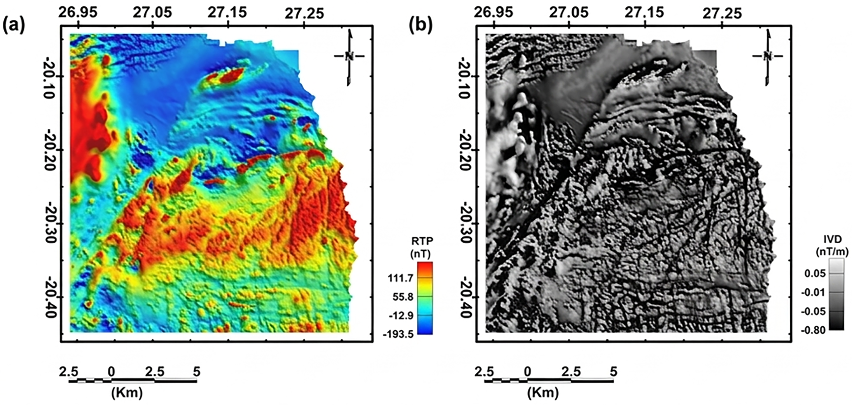
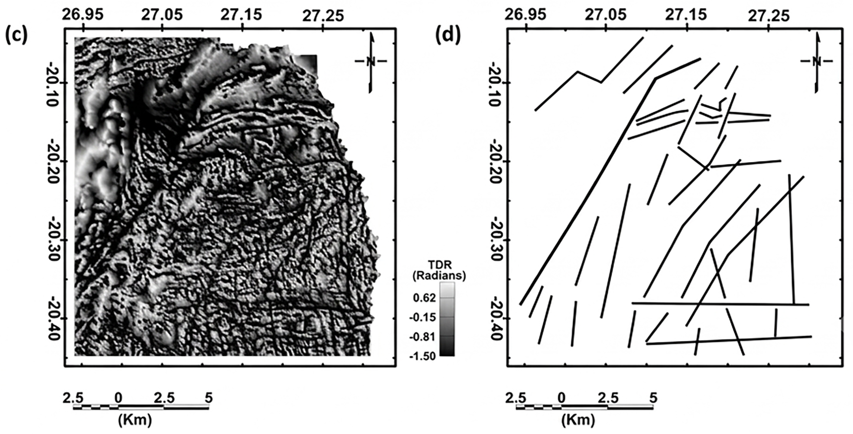
Figure 4: Enhanced aeromagnetic maps after applying the various filters: (a) Reduce to pole (RTP), (b) first vertical derivative of RTP, (c) tilt derivative of RTP, and (d) delineated lineaments showing a major trend in NE–SW direction.

The mapped maps reveal that the predominant structural trend is NE–SW, with N–S, and a lesser E–W, trend. The narrow linear magnetic anomalies have been interpreted as dyke-like features, and darker discontinuities on the derivative maps as faults, shear zones and fractures. The termination of a distinct NE–SW high magnetic domain of the Maitengwe greenstone belt against an evident major NE–SW shear structure is highlighted in Fig. 4a [41]. The same truncation patterns are seen in the northern part of Fig. 4a–c, with a possible dextral displacement. Further, non-magnetic lineaments trending towards the northeast cut across the magnetic units and are seen as the sharp junctions between magnetic bands, suggesting fault or fracture zones as possible pathways for the movement of hydrothermal fluids and related mineralisation. The anomalies with broad curvilinear high amplitude are believed to be ironstone units while the circular magnetic highs are considered to be basic and ultrabasic intrusive bodies [41].

After the interpretation, the lineaments were digitized with map tool extension of the software Oasis Montaj. The final interpretation of the structural lineament map is presented in Fig. 4d and this interpretation was used to select the exploration target shown in Fig. 5.

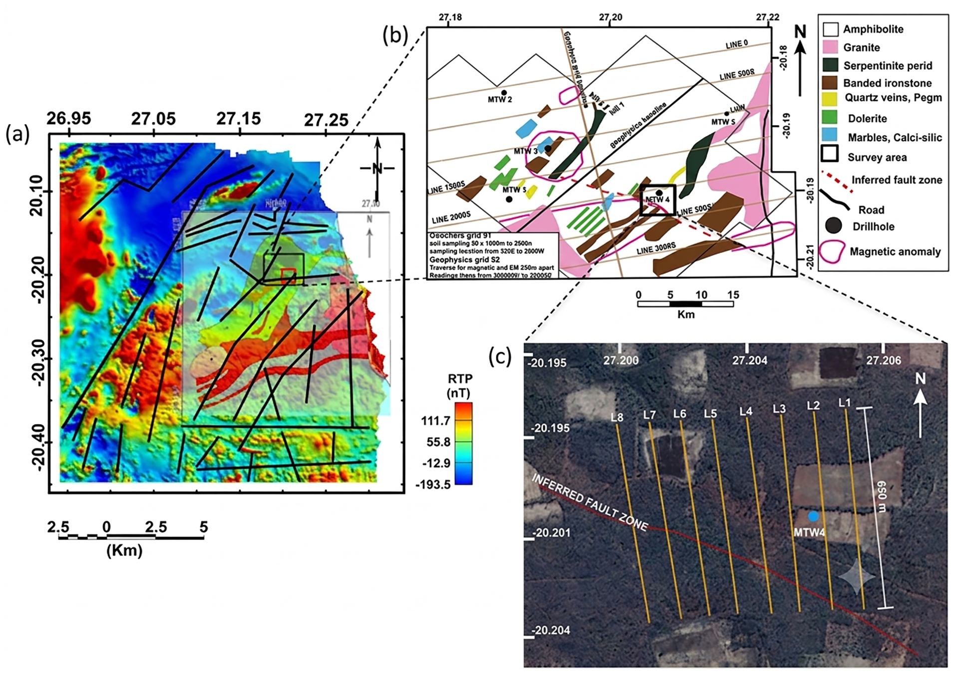
Figure 5: Survey design (a) reduced-to-pole (RTP) aeromagnetic map showing the present survey area (red rectangle) and the previous survey area (black rectangle). (b) Previous geophysical survey grids and drillhole locations (black dots), including borehole MTW4 within the selected study area. (c) Induced polarization–electrical resistivity imaging (IP–ERI) survey lines (L1–L8) oriented in the NW–SE direction.

The lineament digitisation was done by hand by using the map tool extension in Oasis Montaj software. Manual interpretation added some subjectivity, but the dominant NE-SW trend was interpreted by many interpreters and only lineaments that were clearly expressed on all three derivative grids (RTP, 1VD, and TDR) were kept for analysis.

2.3 IP–ERI Data Acquisition and Processing

The Induced Polarization–Electrical Resistivity Imaging (IP–ERI) method was used to characterize subsurface electrical resistivity and chargeability simultaneously. In this method, current is injected into the ground through a pair of current electrodes, while the resulting potential difference is measured between non-polarizable potential electrodes. Apparent resistivity (ρa) is then determined from Ohm’s law using the measured potential difference, injected current, and the geometric factor of the electrode array [42,43]. Because sulphide mineralization may produce a weak resistivity contrast but a distinct polarization response, the joint use of resistivity and chargeability provides a more reliable basis for identifying mineralized zones than resistivity alone [44,45]. Machine learning approaches have recently been developed for efficient inversion of induced polarization parameters, significantly reducing computational cost while producing reliable inversion results comparable to traditional methods [46]. Table 1 summarizes the acquisition and inversion parameters used for the IP–ERI survey, including survey geometry, instrumentation, data acquisition settings, and inversion specifications.

In this study, IP measurements were acquired in the time domain, where the decay of secondary voltage is recorded after current cut-off. During current injection, the measured primary voltage (VP) is used in resistivity estimation, whereas after interruption of the current, the decaying secondary voltage reflects the temporary storage and release of electrical charge within the subsurface [44]. Since voltage cannot be measured reliably at the exact instant of current interruption due to switching transients [43], the decay response is sampled over a finite time window after cut-off. The apparent chargeability is therefore defined from the normalized area under the decay curve over the interval (t1,t2), as illustrated in Fig. 6, and may be written as

mc=1VP∫t1t2Vtdt(9)

where Vt is the measured decay voltage at time t, and mc has units of time, commonly reported in milliseconds [47].

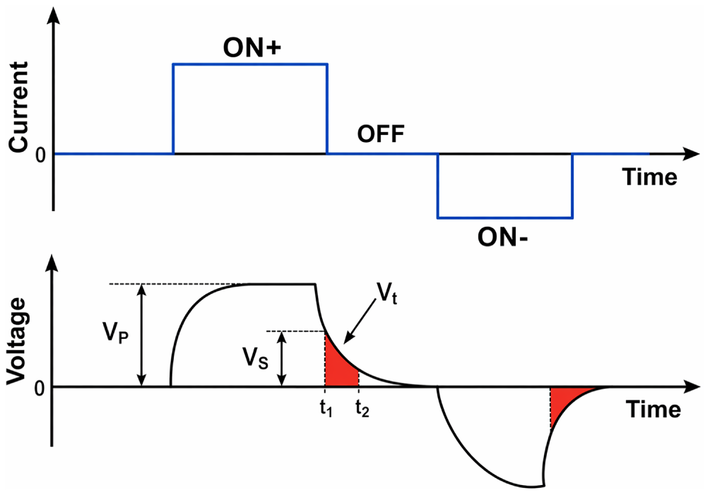
Figure 6: Time domain waveform [47].

Note: In this study, all chargeability values are reported in millivolts per volt (mV/V). For the time-domain induced polarization (IP) system employed (VIP 5000 with a 4 s ON–OFF waveform and an initial delay time of 0.2 s), 1 mV/V is equivalent to 1 ms of integrated decay voltage normalized to the primary voltage. Consequently, the chargeability range of 1.8–10.7 mV/V reported in this study corresponds to 1.8–10.7 ms.

The IP–ERI survey was carried out using a VIP 10,000 three-phase voltage-regulated motor generator coupled to a VIP 5000 current-regulated time-domain transmitter and an Elrec Pro 10-channel receiver in Fig. 7. The same system was used to acquire both apparent resistivity and apparent chargeability data. Current was injected through stainless-steel electrodes, and saltwater was applied around the current electrodes to reduce electrode–ground contact resistance. The potential difference was measured using non-polarizable porous-pot electrodes filled with saturated Copper II sulphate solution because of their low and stable electrode polarization response [45,48]. The ground resistance around the receiving electrodes was maintained below 1 kΩ using wet muddy soil where necessary.

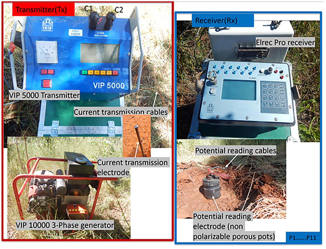
Figure 7: IP–ERI geophysical equipment was employed in the survey.

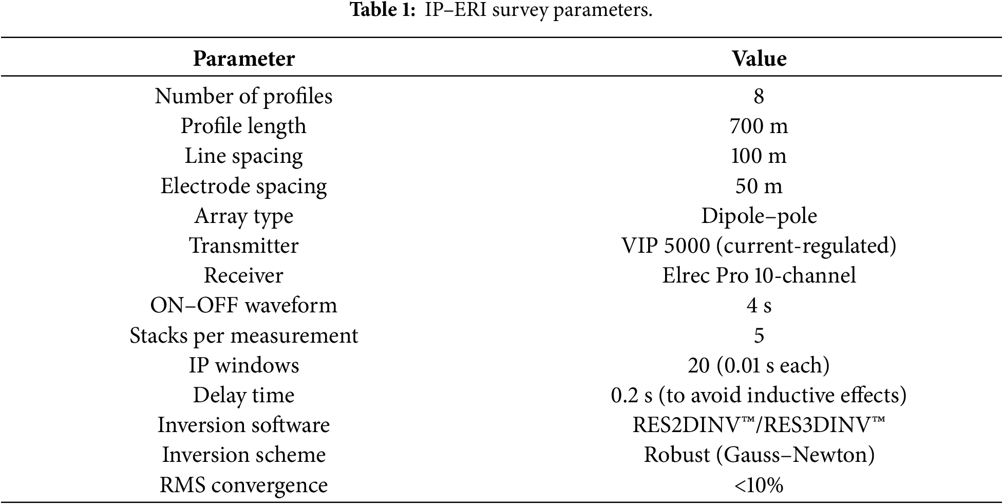
To reduce capacitive and inductive coupling, current and potential cables were separated by at least 1 m or crossed at right angles where required [49,50]. The survey consisted of eight profiles, each 700 m long, with 100 m line spacing and 50 m electrode spacing in Fig. 5. The lines were oriented NW–SE to cut across the main lithological trend. A dipole–pole array was selected because of its favorable depth of investigation, lateral coverage, and lower sensitivity to telluric noise [42]. The current electrode was positioned with a −50 m offset from the first potential electrode, while the potential electrodes were connected to the receiver through a multi-electrode cable.

Acquisition parameters were: 4 s ON—OFF waveform, 5 stacks per measurement, and 20 IP windows, each 0.01 s long. Only the decay part of the response after a delay of 0.2 s was used for the chargeability analysis to avoid the early-time inductive effects. Outliers due to instrumental effects and background noise were filtered from the acquired data in the software Prosys II. The filtered data sets were then inverted using RES2DINV™ and RES3DINV, which discretize the subsurface into rectangular cells and discretely estimate distributions of resistivity and chargeability values that are compatible with the measured data [51].

The standard Gauss–Newton least-squares scheme was used for model inversion in double precision according to [51,52]. Initial damping factor was set to 0.1 and the minimum damping factor was set to 0.007, and a first-layer damping factor was used to suppress near surface rippling which was caused by sparse coverage, which was set to 5.0. A good inversion algorithm was chosen to enhance the representation of sharp electrical contrasts in the subsurface [53]. Since topographic correction was not needed the fine-mesh finite-difference forward model was adopted and a maximum of 7 iterations was used with a convergence limit of 1%. The models were evaluated by the root mean square (RMS) misfit between measured and calculated responses and models whose RMS error is less than 10% were considered as acceptable models.

2.4 Physics-Informed Machine Learning Framework (GeoPhysML)

The inversion results were subsequently used to create the GeoPhysML framework to estimate the probability of sulphide mineralization based on combined aeromagnetic and IP–ERI attributes. In this workflow, geophysical inversion is used to complement machine learning. The inversion stage is used to obtain the spatial distribution of physical properties, mainly resistivity and chargeability, whereas the learning stage is employed to discover patterns of physical properties, including the magnetic derivatives, related to mineralized zones. The goal is not to replace the inversion, but to incorporate its outputs into a predictive model that is based on geophysical behaviour. Physics-informed neural network frameworks have recently been validated for solving both forward and inverse geophysical problems, supporting regularization approaches in geophysical inversion [54].

The prediction mission was defined as a managed binary classification process of mineralized and non-mineralized grid units. The labels on the training were associated with the interval of the borehole, and a geophysical cell was associated with each spatial label. Intervals where sulphide mineralization was confirmed were identified as positive and intervals without evidence of sulphide mineralization were identified as negative. This enabled the model to learn the geophysical signature of mineralized zones but also to have direct geophysical control from borehole observations.

GeoPhysML aimed to capture the nonlinear relationship between fused geophysical attributes and the mineralization likelihood and to bias the prediction based on physically meaningful regularization terms. The framework therefore combines spatially collocated magnetic and IP–ERI features, borehole-based supervision, and geophysical constraints within a single prediction model for sulphide targeting.

2.4.1 Model Architecture

Let the labelled dataset be defined on a common spatial grid as

𝒟={(xi,yi,ρi,mc,i)}i=1n,(10)

where n is the number of labelled grid cells, xi∈Rd is the feature vector at the i-th cell, yi∈{0,1} is the binary mineralization label, ρi is the inverted resistivity, and mc,i is the inverted chargeability. In this study, the input vector is

xi=[Ti, TRTP,i, T1VD,i, TTDR,i, ρi, mc,i]⊤,(11)

where Ti denotes the total magnetic intensity, TRTP,i is the reduced-to-pole response, T1VD,i is the first vertical derivative, and TTDR,i is the tilt derivative at the same spatial location.

For compact notation, the feature matrix and target vectors are written as

X=[x1⊤x2⊤⋮xn⊤]∈Rn×d,y=[y1y2⋮yn]∈Rn,(12)

with analogous vectors ρ∈Rn and mc∈Rn for resistivity and chargeability [55].

GeoPhysML was formulated as a feed-forward neural network with a shared hidden representation and three output branches. The shared encoder maps each input vector xi into a latent representation hi(l) through successive affine transformations and nonlinear activations:

hi(0)=xi,(13)

hi(l)=ϕ(W(l)hi(l−1)+b(l)),l=1,2,…,L,(14)

where W(l) and b(l) are the weight matrix and bias vector of the l-th hidden layer, respectively, and ϕ(⋅) is the rectified linear unit (ReLU),

ϕ(z)=max(0,z).(15)

The final shared hidden state hi(L) is then passed to three separate output heads [55]. The first head estimates the mineralization probability

p^i=σ(wp⊤hi(L)+bp),(16)

where σ(⋅) is the sigmoid activation function,

σ(z)=11+e−z,(17)

so that 0≤p^i≤1. The quantity p^i is interpreted as the predicted probability that the i-th grid cell belongs to a mineralized zone.

The second and third heads estimate auxiliary physical fields:

ρ^i=wρ⊤hi(L)+bρ,(18)

m^c,i=wm⊤hi(L)+bm.(19)

Accordingly, the network maps each feature vector into the triplet

fθ:xi↦(p^i,ρ^i,m^c,i),(20)

where θ denotes the set of all trainable parameters in the shared encoder and the three output branches. This is prominent as the mineralization probability is the primary target, whereas ρ^i and m^c,i are the auxiliary physically restricted outputs that regularize the common representation [55].

Note on Auxiliary Outputs: Although resistivity (ρ) and chargeability (mc) are included as input features, the auxiliary prediction heads serve a fundamentally different purpose. The input values represent observed physical properties obtained from geophysical inversion, whereas the auxiliary outputs correspond to the network’s predictions of these same properties. By minimizing the data-misfit terms (Lρ,data and Lm,data) together with the spatial regularization terms (Lρ,smooth and Lm,grad), the shared encoder is encouraged to learn latent representations that are not only discriminative for mineralization prediction but also consistent with the spatial behavior of the underlying geophysical fields. This approach is not circular; rather, it represents a form of multi-task learning in which the auxiliary tasks act as regularizers, guiding the shared representation toward geophysically plausible solutions and improving model generalization.

2.4.2 Physics-Informed Regularization

The restraints were applied to the auxiliary outputs of resistivity and chargeability, moderately than to the individual mineralization label completely. This approach maintains the distinction between the two goals of classification and geophysical regularization. Specifically, the resistivity and chargeability are supposed to be smooth within a geological domain but may present singular variations at the boundaries of structures and alteration zones. The regularization, therefore, was constructed to suppress implausible spatial variability while being able to capture spatial variation consistent with the inversion results.

For the mineralization branch, the prediction loss was defined using binary cross-entropy:

ℒcls=−1n∑i=1n[yilog⁡(p^i)+(1−yi)log⁡(1−p^i)].(21)

To constrain the auxiliary resistivity prediction, a data-misfit term and a Laplacian smoothness term were introduced [56]. The resistivity data-misfit is

ℒρ,data=1n∑i=1n(ρi−ρ^i)2(22)

Let Ω denote the spatial grid over the survey area. The Laplacian operator applied to the predicted resistivity field ρ^(s), with s=(x,y,z), is

∇2ρ^=∂2ρ^∂x2+∂2ρ^∂y2+∂2ρ^∂z2.(23)

The associated smoothness penalty is written as

ℒρ,smooth=1|Ω|∑s∈Ω(∇2ρ^(s))2,(24)

which suppresses spurious short-wavelength fluctuations in the learned resistivity field [57].

For chargeability, the regularization was defined using a gradient-matching term rather than a divergence term, because chargeability is treated here as a scalar field. The chargeability data-misfit is

ℒm,data=1n∑i=1n(mc,i−m^c,i)2,(25)

and the spatial gradient of the predicted chargeability field is

∇m^c=[∂m^c∂x,∂m^c∂y,∂m^c∂z]⊤.(26)

The gradient-consistency penalty is then defined as

ℒm,grad=1|Ω|∑s∈Ω‖∇mc(s)−∇m^c(s)‖22.(27)

Combining Eqs. (21)–(27), the total objective function becomes

ℒ(θ)=ℒcls+α1ℒρ,data+α2ℒρ,smooth+α3ℒm,data+α4ℒm,grad,(28)

where α1,α2,α3,α4≥0 are weighting coefficients controlling the contribution of the auxiliary physical constraints relative to the classification objective [58–60].

The structure of Eq. (28) follows a clear sequence. The term ℒcls forces the network to separate mineralized from non-mineralized cells. The terms ℒρ,data and ℒm,data ensure that the auxiliary outputs remain consistent with the inverted resistivity and chargeability fields. The spatial regularization terms ℒρ,smooth and ℒm,grad encourage spatial smoothness of the auxiliary fields, and therefore stabilise the feature space learned by the shared encoder. Thus, the model is not only trained on the class labels, but also on the spatial behaviour of the underlying geophysical fields that are used to determine the labels.

The geological context is also imposed by the borehole-driven labels, structural interpretation of the magnetic derivatives and the co-located resistivity and chargeability data. As a result, the regularization is not applied in a vacuum, but in conjunction with the training set that already takes into account the lithological and structural context of the Maitengwe Greenstone Belt. Table 2 summarizes the architecture, training parameters, software environment, and computational resources used for the development and optimization of the GeoPhysML model.

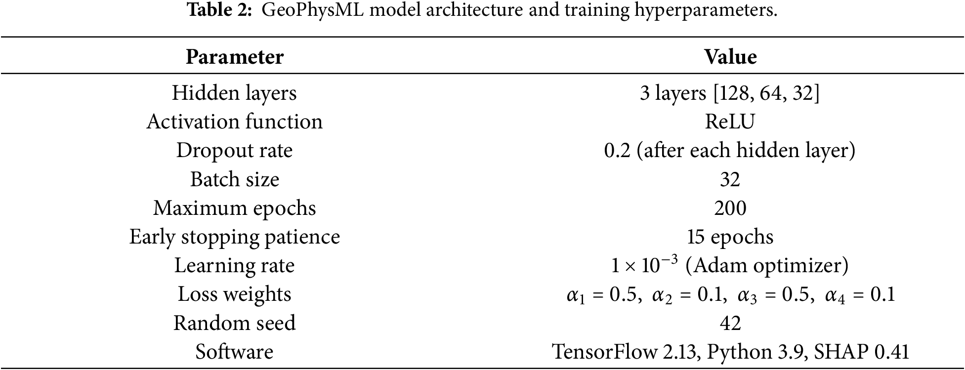
2.4.3 Spatial Blocking for Data Splitting

To prevent spatial autocorrelation from artificially inflating model performance metrics, a spatial blocking strategy was implemented during dataset partitioning. The survey area was divided into blocks measuring 200m×200m, and each block was assigned exclusively to either the training, validation, or test dataset. A minimum separation distance of 100m was maintained between training and test blocks to minimize spatial dependence between the datasets.

This approach ensures that neighboring grid cells, which may exhibit similar geophysical responses due to spatial continuity, are not simultaneously included in both training and testing datasets. Consequently, the resulting performance metrics provide a more realistic assessment of the model’s ability to generalize to previously unseen areas. The spatial block assignments used for dataset partitioning are summarized in Table 2.

The grid was defined using a common three-dimensional (3D) geophysical framework shared by both borehole and spatial datasets, consisting of voxels measuring 25m×25m×10m. Labelled grid cells were generated by spatially intersecting borehole mineralization logs with the common 3D geophysical grid. A voxel was assigned a positive label (mineralized) only when the corresponding depth interval intersected a sulphide-bearing zone containing ≥5% disseminated pyrite and quartz–carbonate veining (MTW1: 110–160 m; MTW2: 118–153 m). Voxels overlapping barren intervals, defined as containing no sulphides or less than 1% trace sulphides, were assigned negative labels. No horizontal buffer was applied during the labelling process; only voxels directly intersected by the borehole trajectory were assigned labels. Borehole MTW4 was excluded from the training dataset and reserved exclusively for independent model validation. To maintain a conservative labelling strategy, ambiguous intervals and zones exhibiting only weak mineralization were classified as negative samples.

2.4.4 Training Algorithm

Model training was carried out using mini-batch optimization with the Adam algorithm and learning rate η=10−3. At each iteration, the network received a batch of collocated geophysical features and produced three outputs: the mineralization probability p^, the auxiliary resistivity prediction ρ^, and the auxiliary chargeability prediction m^c. The trainable parameters θ were then updated by backpropagation to minimize the total objective function in Eq. (28).

For a mini-batch ℬ⊂𝒟, the update step can be written as

θ(t+1)=θ(t)−ηAdam(∇θℒℬ(θ(t))),(29)

where ℒℬ denotes the batch-wise form of the total loss and t is the iteration index. The batch loss consists of the classification term together with the auxiliary resistivity and chargeability penalties:

ℒℬ=ℒclsℬ+α1ℒρ,dataℬ+α2ℒρ,smoothℬ+α3ℒm,dataℬ+α4ℒm,gradℬ.(30)

Training was performed for a maximum of Nepochs epochs. During each epoch, the mini-batches were processed sequentially, the batch loss was evaluated, and gradients were propagated through both the shared encoder and the three output branches [61,62]. Validation performance was monitored after each epoch, and the learning rate was reduced when the validation loss plateaued. The final model parameters correspond to the checkpoint with the lowest validation loss.

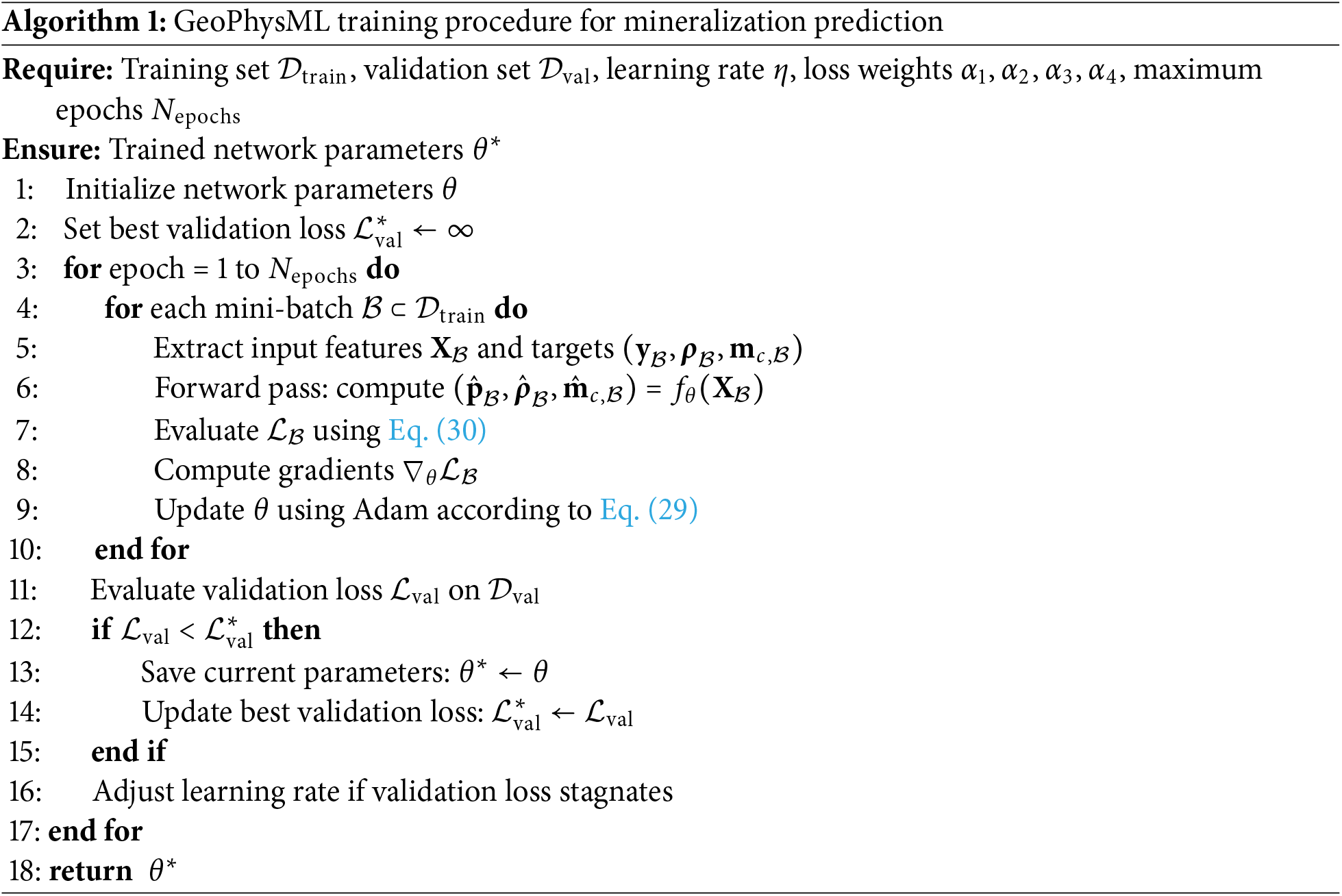
The complete GeoPhysML training procedure is summarized in Algorithm 1, which outlines the forward pass, loss computation, gradient backpropagation, and validation monitoring steps.

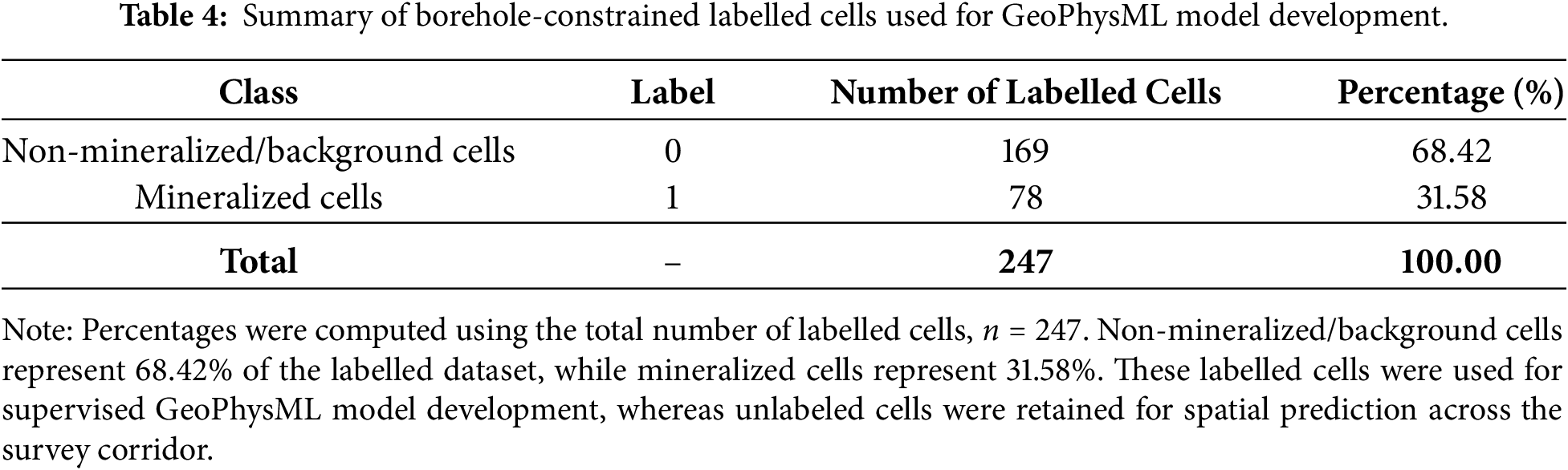
To evaluate predictive generalization, the labelled dataset was divided into training and test subsets using a stratified split so that the proportion of mineralized and non-mineralized cells was preserved in both sets. In addition, the partition was checked spatially to reduce direct neighbourhood overlap between training and test samples, thereby limiting performance inflation caused by short-range spatial autocorrelation. Model evaluation was then carried out only on the held-out test set using classification-based performance measures. Table 3 summarizes the borehole-constrained labelled cells used for GeoPhysML model training.

Borehole MTW4 was used ONLY for independent validation of the final model predictions. It was NOT included in the training set. The positive labels are derived from MTW1 and MTW2. This ensures independence between training and validation.

Training/Validation/Test Split (Spatial Blocking):

•   Training set: 173 cells (70%)

•   Validation set: 37 cells (15%)

•   Testing set: 37 cells (15%)

Supervised labels were assigned from borehole-constrained mineralization intervals between mineralization intervals within the mineralization target stratigraphic units of the study area. Cells that intersected intervals where sulphide mineralization was confirmed were considered positive, while cells that intersected intervals where there was no evidence of sulphide mineralization were considered negative. The labels were moved to the common geophysical grid at cell level to yield the set of samples that were mineralized and non-mineralized to develop and test the model. Table 4 provides a summary of the borehole labeling scheme.

Intermissions with the greatest combined evidence for sulphide enrichment, alteration, and structurally controlled veining were supposed positive labels, and intervals with only trace to moderate sulphides were not assigned to the positive class to avoid overestimation.

The data partitioning approach was a combination of two complementary approaches. To reduce the spatial effect, the survey area was divided into 200 m × 200 m blocks and the minimum separation distance between the training and test blocks was set to be 100 m. This procedure will reduce the impact of spatial autocorrelation and avoid over-optimistic results due to the spatial overlap of samples.

Second, stratified sampling was used within the spatially defined subsets to ensure the mineralized cells (31.58%) and non-mineralized cells (68.42%) are represented at a similar proportion in the training, validation and test sets. The two-stage partitioning strategy maintains both spatial independence and class balance of the 70/15/15 dataset split reported in the abstract, which gives a better sense of performance of the model in generalizing.

2.4.5 Data Fusion and Feature Matrix Construction

The aeromagnetic and IP–ERI datasets were fused on a common spatial framework to produce the input matrix used by GeoPhysML. All datasets were first projected to WGS 84 UTM Zone 35S to ensure positional consistency. The aeromagnetic grids, originally provided at 50 m resolution, were then resampled to match the spatial support adopted for the IP–ERI model.

The IP–ERI inversion outputs, namely resistivity ρ and chargeability mc, were exported from RES3DINV as XYZ data referenced by easting, northing, and depth. These values were interpolated within the survey limits onto a regular three-dimensional grid with voxel size 25 m×25 m×10 m using nearest-neighbour assignment. Once the IP–ERI grid had been established, the aeromagnetic attributes were collocated at the same voxel locations. The resulting feature vector at each grid cell was defined as

xi=[Ti, TRTP,i, T1VD,i, TTDR,i, ρi, mc,i]⊤,(31)

where Ti is the total magnetic intensity, TRTP,i is the reduced-to-pole response, T1VD,i is the first vertical derivative, TTDR,i is the tilt derivative, and ρi and mc,i are the collocated resistivity and chargeability values, respectively.

To place all variables on a comparable scale before training, each feature was standardized using the statistics of the training subset only:

xnorm=x−μxσx,(32)

where μx and σx denote the mean and standard deviation of feature x computed from the training data [55]. This prevented leakage of information from the test set into the normalization stage. Grid cells lying outside the IP–ERI survey extent were excluded from the fused dataset. The small number of remaining cells with incomplete feature values (<0.1%) were imputed using k-nearest neighbours with k=3 based on spatial proximity.

The final feature matrix X therefore had dimension N×6, where N is the number of valid grid cells within the survey area. Of these, 247 cells were labelled from borehole-controlled intervals and 1284 remained unlabeled for subsequent spatial prediction.

Ablation Study Design

To isolate the contribution of the physics-informed components of GeoPhysML, an ablation study was designed using three neural-network variants trained and evaluated under the same data partition and optimization settings. The first variant was a baseline multilayer perceptron (MLP) trained only for binary mineralization classification from the fused geophysical feature set. The second variant extended the baseline network by introducing auxiliary resistivity and chargeability output branches, but without physics-informed regularization. The third variant was the full GeoPhysML model, which included both the auxiliary physical-property outputs and the physics-informed loss terms defined in Eq. (28). This staged comparison was intended to distinguish the effects of the base neural architecture, the auxiliary multi-output structure, and the physics-informed regularization on predictive performance.

2.5 Limitations of Pseudo-3D Interpolation

The pseudo-3D interpolated reconstruction was constructed by combining eight parallel 2D profiles, spaced 100 m apart. While such a model can be used to illustrate lateral continuity, it is important to consider the interpretational constraints.

First, the cross-line resolution is limited by the 100 m line-spacing. This means that structures less than about 50–70 m in that direction might not be adequately resolved. Second, the pseudo-3D reconstruction is somewhat based on interpolation between profiles. The resistivity and chargeability between lines were interpolated by a minimum-curvature approach, which can result in blurring of boundaries and apparent continuity where there are no measurements. Third, the survey layout is anisotropic: the spatial resolution is higher along the profiles (electrode spacing is 50 m) than across them (line spacing is 100 m). As such, features trending NE–SW, which are more parallel to the survey geometry, are likely to be better interpreted than those that are perpendicular to the profiles. Finally, the effective resolution of the 700 m-long spread is about 200 m depth, which is consistent with the primary mineralised zone in borehole MTW4 at 118–153 m depth.

These factors indicate caution while estimating geometric continuity outward from the profiles, but they are not sufficient to rule out the results of pseudo-3D interpretation. Therefore, instead of being employed exclusively for geological analysis, the pseudo-3D findings were combined with drill data, magnetic structure, and machine-learning prediction.

3  Results and Discussion

The results are presented in two steps. First, resistivity and chargeability inversions are discussed to establish the geoelectrical setting of the area surveyed, and its correlation with the MTW4 borehole log. Then, the machine learning results are examined to assess whether the integrated GeoPhysML approach enhances spatial delineation of interpreted mineralization. Thus, the focus of discussion is the geoelectrical properties of the subsurface zones, their relation to the borehole control, and the influence of the predictive model on improving geological target delineation.

Interpretation of the inverted sections was aided by the stratigraphy of borehole MTW4 (Fig. 8), which is near the survey lines and is the primary subsurface control for correlation of lithology and mineralization. In the inverted sections, the resistivity ranges from 15.6 to 3053 Ω m and the chargeability from 1.8 to 10.7 mV/V. The 2D and pseudo-3D reconstruction together reveal three electrical domains that are common throughout the sections: a shallow low-response zone, an intermediate zone of moderate electrical contrast and a deep zone of high resistivity and chargeability. These regions show a vertical transition between weathered and weakly mineralised rocks at the surface to more altered and sulfur-bearing rocks at deeper levels.

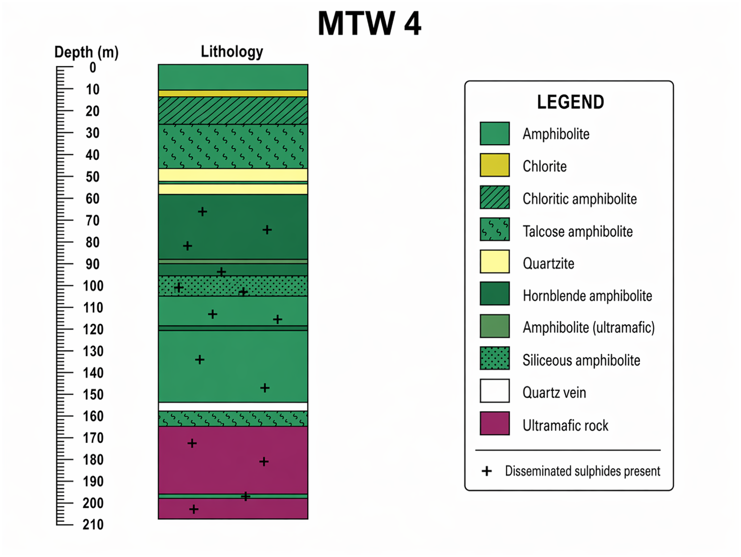
Figure 8: Borehole log MTW4 is located in the vicinity of the survey lines in the study area. A weathered zone extends from the surface into the chloritic amphibolite. Quartzite and hornblende amphibolite are observed from depths of 27 to 95 m; the latter exhibits minor alteration, quartz and carbonate veining, and disseminated sulphides occurring as blebs, smears, and stringers along fractures enriched with quartz veins. At a depth of 99 m, the amphibolite contains high (5%) disseminated sulphides (pyrite and pyrrhotite). Extensive alteration, indications of folding and shear zones, and disseminated sulphides enriched along veins are noted between 118–153 m. A possible fracture or fault is observed at a depth of 156 m [32].

For consistency, the anomalies in chargeability are referred to as zones A–C and those in resistivity as zones I–III. Low to moderate chargeability (zones A–B) and low to moderate resistivity (zones I–II) represent weathered chloritic and talcose amphibolite. Zones B and II–III are moderate chargeability and resistivity and have been determined as dense quartzite/hornblende rich rocks containing disseminated sulphides. The most significant is the overlap of zone C and zone III showing high chargeability with high resistivity. This is more likely to be a highly silicified amphibolite with quartz–carbonate veining and disseminated metallic sulphides as opposed to barren resistive formations in the geology of the Maitengwe Greenstone Belt. This is confirmed by the MTW4 borehole record which reflects alteration, veining and enrichment of sulphides in the deeper interval shown in Fig. 8.

Eight 2D resistivity and chargeability inversions of the IP-ERI profiles were compiled in RES2DINV and a pseudo-3D ERI/IP volume was constructed in RES3DINV, stacking the parallel 2D sections. The pseudo-3D horizontal sections (Figs. 9–12) were used to assess the continuity and geometry of the inverted anomalies that may be obscured in the 2D sections [63]. To simplify the discussion, we only selected four representative profiles (Profiles 4, 5, 6 and 8) for discussion (Figs. 9 and 11), whereas the other profiles are included in the pseudo-3D reconstruction (Figs. 10 and 12). The depth of the 2D sections is up to about 215 m, and inversion errors are acceptable, with RMS errors for resistivity less than 8% and for chargeability less than 0.6%.

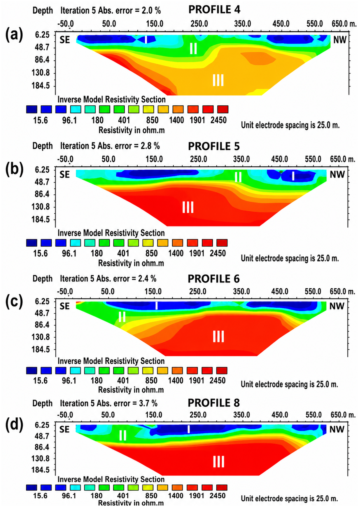
Figure 9: 2D resistivity inverted models: Profile 4 (a), Profile 5 (b), Profile 6 (c), and Profile 8 (d). Vertical and horizontal axes represent depth and distance along the profile, respectively. The colour scale below the profiles represents different resistivity values.

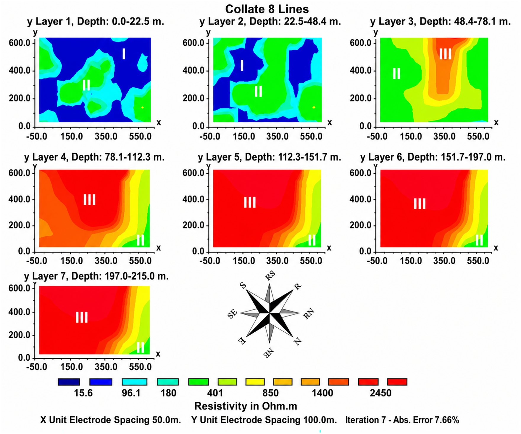
Figure 10: Horizontal (x–y) depth slices of the pseudo-3D resistivity model produced by collation of 2D profiles and interpolation of resistivity data. The depth of view is indicated at the top of each plane, and the compass shows the orientation of the profiles and their anomalies.

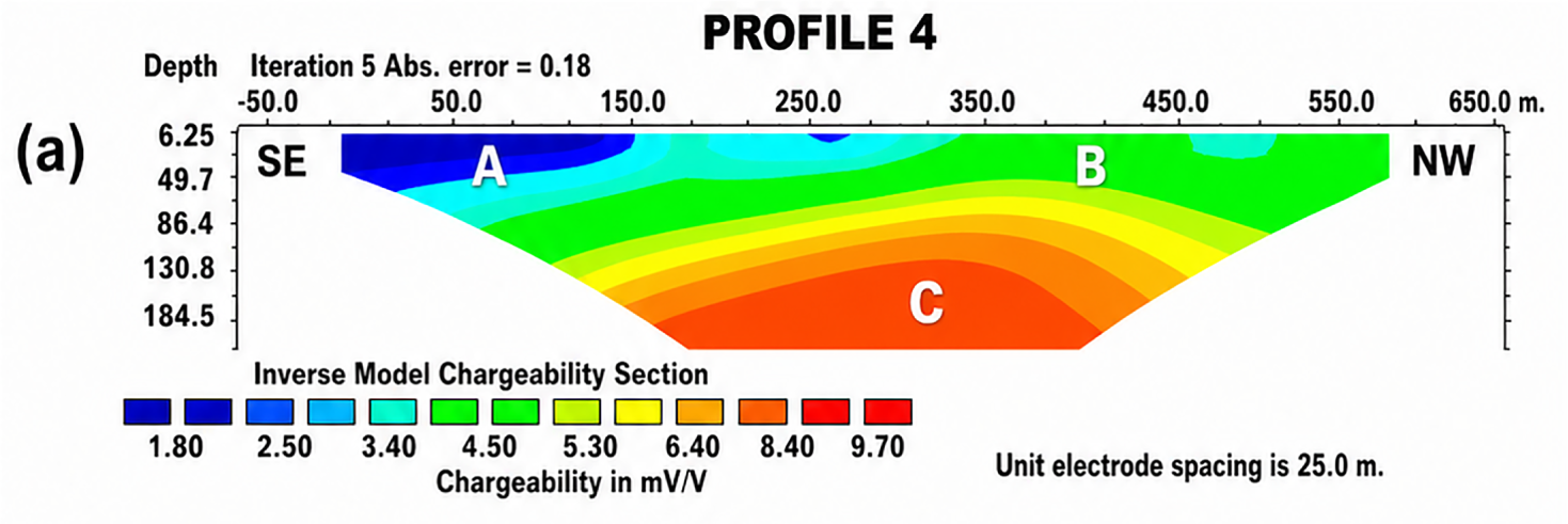
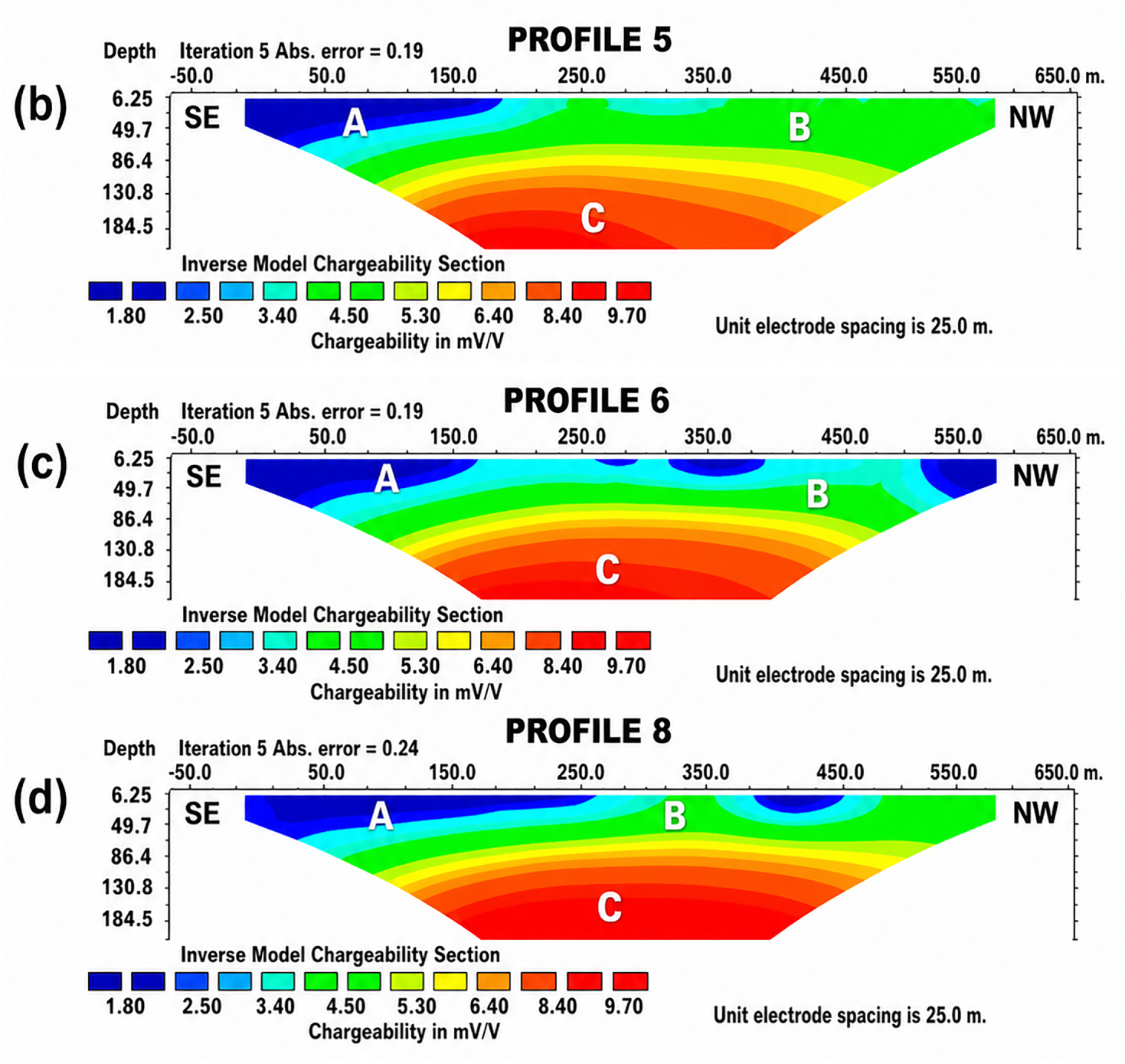
Figure 11: 2D IP inverted models: Profile 4 (a), Profile 5 (b), Profile 6 (c), and Profile 8 (d). Vertical and horizontal axes represent depth and distance along the profile, respectively.

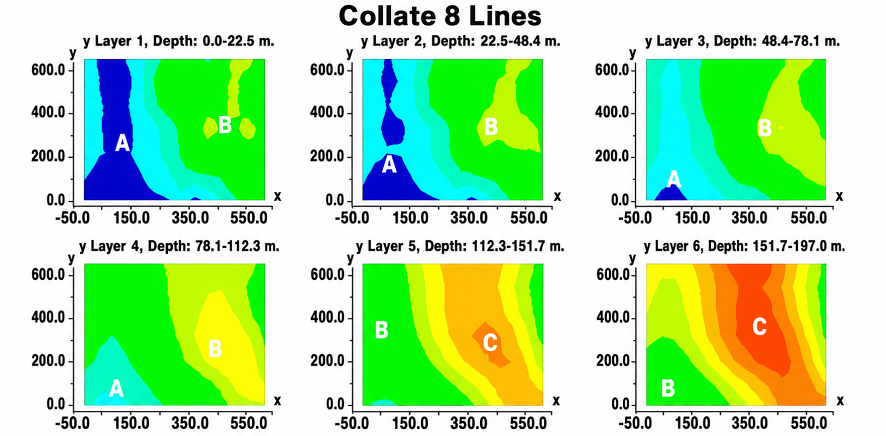
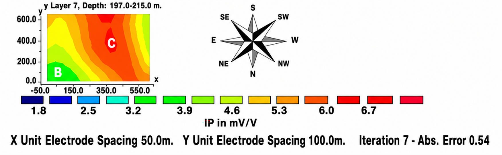
Figure 12: Horizontal (x–y) depth slices of the pseudo-3D chargeability model produced by collation of 2D profiles and interpolation of resistivity data. The depth of view is indicated at the top of each plane, and the compass shows the orientation of the profiles and their anomalies.

Zone I (blue; 15–96 Ω⋅m) is weathered chloritic amphibolite close to the surface. The fractured and moderately altered amphibolite is in Zone II (green–yellow; 180–850 Ω⋅m). Zone III (red; >1400 Ω⋅m) is silicified and competent bedrock and relates to quartz–carbonate veining.

The contrast in resistivity (vertical transition from Zone I to Zone III) is greatest on Profile 5 (Fig. 9b) with a sharp resistivity contrast seen. This sudden change is seen as a fault-bounded contact whereby it is believed that lithological variation and fluid movement in the study area was structurally controlled.

3.1 Interpretation of Electrical Domains

Three reoccurring electrical domains are defined in the resistivity inversion result. Zone III (1400–3053 Ω m) is the deeper, resistive zone, Zone II (180–850 Ω m) is an intermediate zone, and Zone I (15.6–96.1 Ω m) is the shallow, conductive zone. In Fig. 9, the general trend is that resistivity generally increases with depth, with Zone I located in the shallow subsurface, Zone II varying in thickness and at depth and Zone III laterally continuous on most profiles. While there is variability in the geometry of the features across the sections, it is overall consistent with vertical electrical zones and lateral variations in the subsurface. Vertical and lateral variations in the depth and continuity of Zones II and III indicate changes in lithology, alteration and deformation. To better understand the orientation and geometry of these features, pseudo-3D resistivity depth-slice maps were produced, since the 2D sections do not clearly define the features between survey lines.

Horizontal slices of the pseudo-3D resistivity model are shown in Fig. 10. The uppermost slices, layers 1 (0–22.5 m) and 2 (22.5–48.4 m) are dominated by low resistivity (zone I) with only small areas of moderate resistivity. In layer 3 (48.5–78.1 m), the moderate resistivity (zone II) dominates, and a SW-NE trending high-resistivity zone appears at the edge of x=350 m and y=200–600 m. At deeper levels, from layer 4 (78.1–112.3 m) to layer 7 (197.0–215.0 m), a wide zone of high resistivity (III) dominates, and occupies most of the y-axis and mainly within x=0–500 m~, with a thin band of moderate resistivity remaining in the far NW corner. This suggests the lower part of the model is dominated by a laterally extensive resistive feature, implying a structurally-controlled and potentially mineralized subsurface.

Two-dimensional chargeability models are shown in Fig. 11 for Profiles 4, 5, 6, and 8, complementing the resistivity sections in Fig. 9a–d. All sections display a shallow low-chargeability zone (A) of 1.8–2.5 mV/V, which is generally more developed toward the SE parts of the profiles, although local variations occur in Fig. 11c,d. Beneath this, a moderate-chargeability zone (B) of 3.4–5.3 mV/V is present, particularly in the upper portions of Fig. 11a,b. At greater depth, a high-chargeability zone (C) of 6.4–10.7 mV/V appears below about 86.4 m and extends laterally across most of the profiles. This deeper and more continuous response is the most significant chargeability feature in the dataset and, when interpreted together with the resistivity models, is consistent with a laterally persistent sulphide-bearing zone.

Pseudo-3D chargeability depth slices are shown in Fig. 12. The shallow levels, corresponding to layers 1–3 (0–78.1 m), are dominated in the SE part of the model by low chargeability (zone A) with values below 2.5 mV/V. Over the same depth range, moderate chargeability values of about 3.2–5.3 mV/V occur from the central part of the model toward the NW end. At greater depth, layers 4 (78.1–112.3 m) and 5 (112.3–151.7 m) are characterized mainly by a moderately chargeable domain (zone B), which forms a SW–NE-trending band in the NW part of the profiles. In the deepest slices, layers 6 (151.7–197.0 m) and 7 (197.0–215.0 m), a high-chargeability zone (C) becomes more distinct. This zone is mainly restricted to x-distances greater than 250 m and is oriented in the SW-NE direction.

The chargeability observations suggest that the most favorable target is not in the shallow low-chargeability region, but the deeper and laterally broad anomaly, which is outlined by zone C. Combined with the resistivity model, the high chargeability and high resistivity response is important. One might expect sulphide-rich zones to be less resistive in many mineral systems, but, due to hydrothermal alteration and silicification, resistive but chargeable zones are found where quartz–carbonate veins host disseminated metallic sulphides [64,65]. In this study, the coincident zones C and III are therefore interpreted as altered and silicified mineralized zones rather than barren resistive units.

This interpretation is consistent with borehole observations from the Maitengwe greenstone belt. Borehole MTW4 (Fig. 8) records hydrothermal alteration, quartz–carbonate veining, and structurally disturbed amphibolitic units, with sulphide occurrence beginning from about 58 m depth and more intense alteration between 118 and 153 m [32]. The deeper chargeability high is therefore compatible with a structurally controlled mineralized corridor rather than diffuse background polarization. The shallower zones, which exhibit low or moderate values of resistivity and chargeability, are more consistent with weathered chloritic and talcose amphibolite with little or no sulphide deposits [47,64].

The pseudo-3D chargeability reconstruction also helps to understand the distribution of the anomaly. Although the 2D sections (Figs. 9 and 11) suggest that there is deeper chargeable material, the slices in Fig. 12 reveal that the anomaly is a linear trend that is mainly confined to the NW part of the survey area. This trend is consistent with the NE-SW structural fabric inferred from the aeromagnetic data (Fig. 5), suggesting that the sulphide mineralization is related to a shear zone. In this respect, the pseudo-3D chargeability model offers the best geophysical image of the interpreted mineralized zone.

The response is also consistent with other studies that show induced polarization (IP) is more diagnostic of mineralization than resistivity. High-resistive but chargeable vein systems have been observed in metalliferous and hydrothermally altered environments, such as quartz-carbonate veins, and alteration halos around ore bodies [27,48,66–68]. The Maitengwe results are also consistent with this pattern: resistivity defines the host environment and alteration, while chargeability is the stronger diagnostic for disseminated sulphide mineralization in the structurally-defined target area.

3.2 Machine Learning Integration

The 2D and pseudo-3D inversion models were kept as the geophysical reference. The major resistivity and chargeability fields were identified and their association with alteration and sulphide-rich sectors. But the inversion alone did not sufficiently define and “edge” spatial variations in the potential for mineralization for target prioritization, especially where structural complexity and smoothing effects mask local trends. For this reason, the resistivity and chargeability derived from the inversion models were combined with the aeromagnetic attributes and were input into the GeoPhysML models.

3.2.1 Machine Learning-Enhanced Prediction Maps

GeoPhysML was trained on the integrated geophysical attributes, total magnetic intensity (TMI), reduced-to-pole response (RTP), first vertical derivative (1VD), tilt derivative (TDR), resistivity (ρ) and chargeability (mc). The output of the model was a probability map, P(mineralization), across the study area. Fig. 13a shows the mineralization probability map overlaid on the aeromagnetic background map and Fig. 13b shows the uncertainty map in terms of the Uncertainty Index (UI). This combined presentation allows the predicted target corridor to be evaluated together with the spatial stability of the model response.

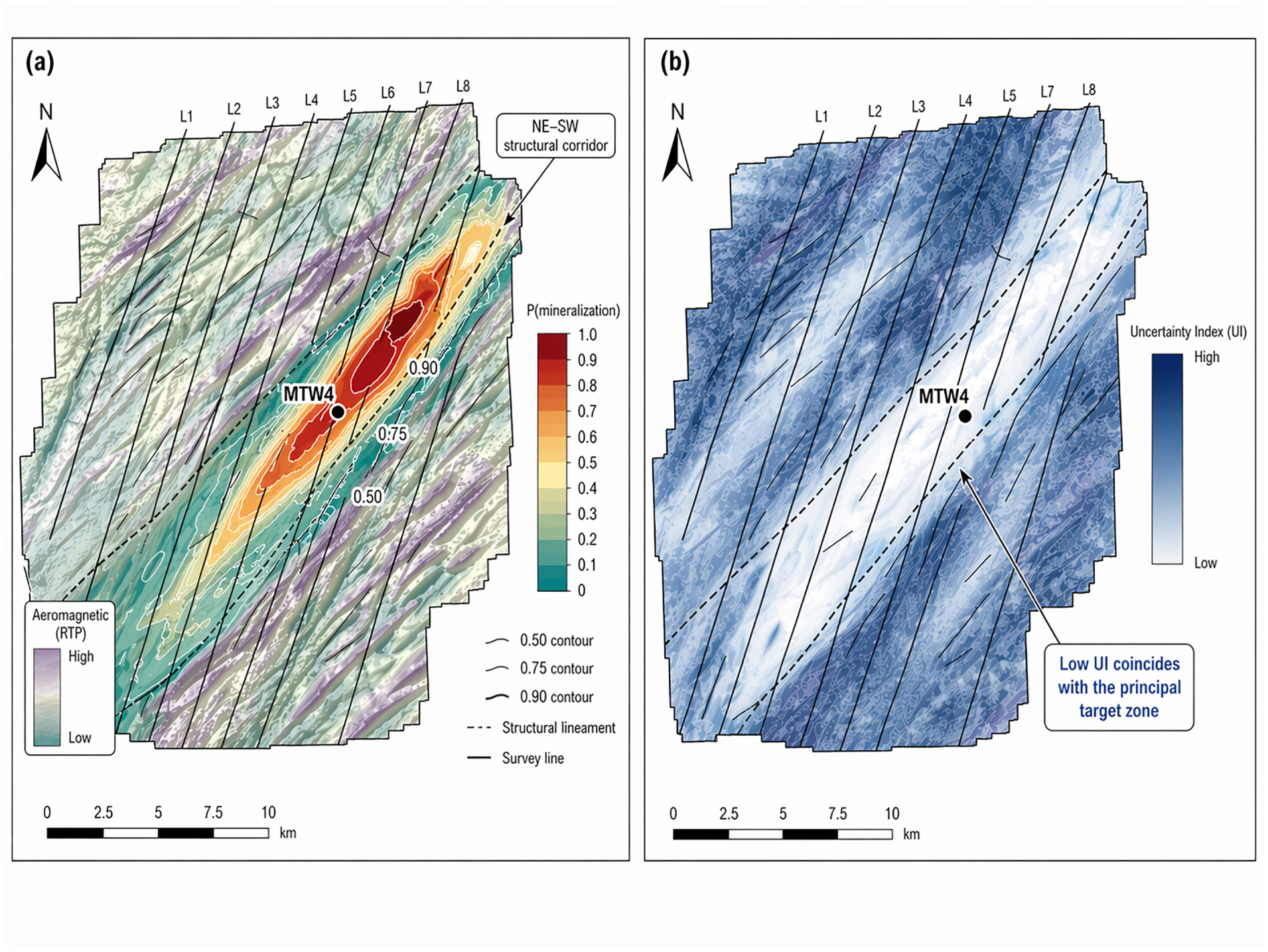
Figure 13: GeoPhysML prediction outputs for Maitengwe greenstone belt. (a) Mineralization prospect map based on the incorporated aeromagnetic and IP–ERI feature set, revealing the main NE-SW target corridor and the position of borehole MTW4. The progressive concentration of the mineralized zone is shown by probability contours. (b) Uncertainty map presented as the uncertainty index (UI), illustrating the relative level of uncertainty in the area of the main mineralization zone compared to the rest of the area of uncertainty.

The magnetic derivatives showed the dominant NE–SW structural grain, with the corresponding high probability zones for mineralization (shown as P(mineralization)>0.75) including the MTW4 location. This spatial agreement suggests that favourable structural setting and geophysical anomaly patterns, not just resistivity or chargeability responses, are the controls on the model response. The probability map thus optimizes the interpretation by the inversion and translates the broad zone of anomalies to mineralization corridors in ranked order. It is important to note that the uncertainty is relatively low in the principal target zone, while the areas around it are likely to contain high uncertainty, and the interpretation of these areas must be made with caution and prudence, as illustrated in Fig. 13b.

The uncertainty map (Fig. 13b) uses the Uncertainty Index (UI), defined as the coefficient of variation the ratio of the standard deviation to the mean of the predicted mineralization probabilities. For each grid cell, UI is computed as:

UI=σdropoutμpred(33)

where σdropout is the standard deviation of the predicted probabilities from 100 stochastic forward passes with dropout enabled, and μpred [69]. The corresponding mean predicted probability is denoted by p^. This ratio normalizes the variability by the magnitude of the prediction, making UI a scale-independent measure of model stability. Lower values (e.g., UI<0.15) indicate high prediction confidence, while higher values reflect greater uncertainty. This formulation is consistent with the coefficient of variation (Eq. (34)) and avoids ambiguity by explicitly stating the division.

3.2.2 Correlation with Borehole Data

The MTW4 borehole log as well as lithology and sulphide data were used to validate the GeoPhysML predictions. The principal high-probability zone (HPZ) (Fig. 13a) is the area where the mineralization prediction probability P(mineralization) is at least 0.75, and it is spatially associated with the MTW4 location and runs along the same NE–SW structural corridor identified through the aeromagnetic interpretation. This target zone is very well correlated to the mineralised borehole interval, which is defined by hydrothermal alteration, quartz-carbonate veins and 5% disseminated sulphides. This local match of the predicted probability anomaly with the borehole controlled mineralized zone provides a local evidence for the GeoPhysML result.

The probability map also helps to focus the interpretation of the geophysical anomaly into a target zone. The model highlights the quadrant in which the favourable electrical responses co-exist with the interpreted structure not just the resistivity or chargeability anomalies. In line with the geological thinking that sulphide mineralization in the Maitengwe belt is structurally controlled and locked up into shear related zones.

The ambiguity map in Fig. 13b is additional piece of evidence that reinforces the spatial confidence of this interpretation. The uncertainty is relatively small in the target corridor around MTW4, implying that the best target area is one of the least uncertain model predictions. Where uncertainty is higher, but still within the main corridor, that indicates an area the prediction is not as well constrained and further IP–ERI coverage or infill drilling would be necessary before the same exploration priority can be given. Fig. 13a,b demonstrates that the mineralization zone predicted by the borehole study and the comparatively well constrained zone are both good contenders.

3.2.3 Uncertainty Index (UI)

The Uncertainty Index (UI) is defined as

UI=σμ(34)

In this case, it is the standard deviation of the mineralization probabilities predicted from 100 Monte Carlo dropout forward passes and the mean predicted probability. Lower UI values (e.g., UI<0.15) signify greater prediction stability and high certainty in the model output, while higher UI values suggest greater uncertainty and may need much more geological, geophysical or drilling information to ensure that the prediction is more reliable.

3.3 Quantitative Model Performance

The accuracy, precision, recall, F1-score, and ROC-AUC were mainly used to evaluate the model’s performance in the classification setting. To quantify the difference between predicted probabilities and a binary label, probability-based error measures were also calculated because GeoPhysML outputs probabilities of mineralization.

The probability error metrics were defined as

MAE=1n∑i=1n|yi−p^i|,(35)

MSE=1n∑i=1n(yi−p^i)2,(36)

RMSE=1n∑i=1n(yi−p^i)2,(37)

where yi∈{0,1} denotes the observed mineralization label and p^i∈[0,1] is the predicted probability of mineralization for the i-th sample.

The classification metrics were computed as

Accuracy=TP+TNTP+TN+FP+FN,(38)

Precision=TPTP+FP,(39)

Recall=TPTP+FN,(40)

F1=2⋅Precision⋅RecallPrecision+Recall,(41)

where TP, TN, FP, and FN denote true positives, true negatives, false positives, and false negatives, respectively.

The results in Table 5 illustrate the stability and reliability of the GeoPhysML model when tested with five different cross validation runs. All the evaluation metrics have small standard deviation (less than 0.65%) which shows that the model predictions are stable and reproducible despite the relatively small labelled dataset.

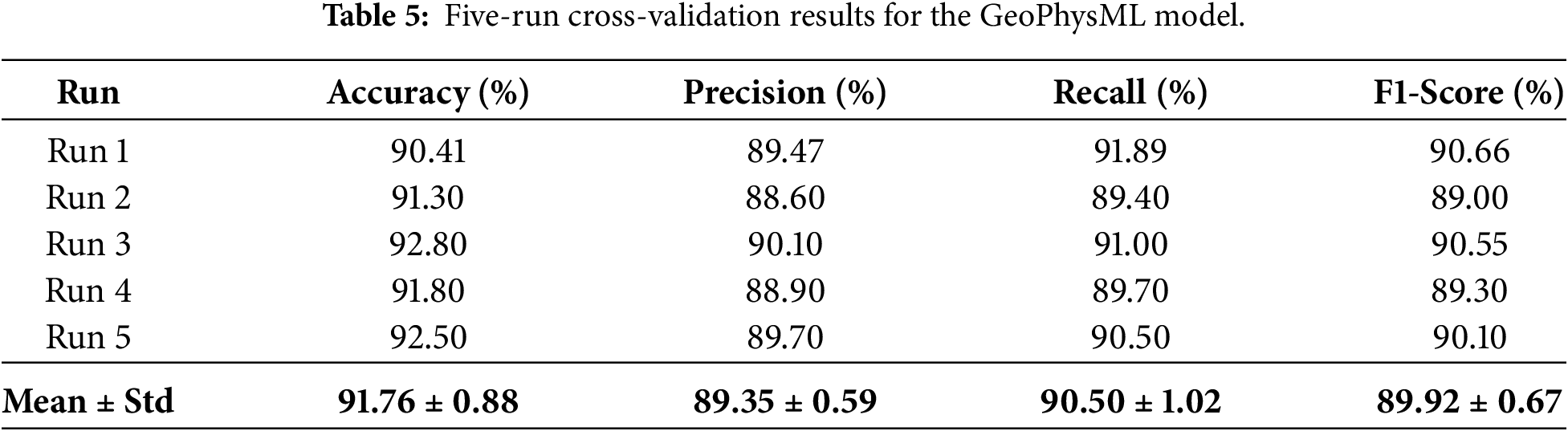
The confusion matrix for Run 1 (Table 6) reveals that there are 3 false negative and 4 false positive in 73 test samples. The results show that the proportion of classification errors is low and that the model can discriminate and classify between mineralized and non-mineralized grid cells. The overall results of the cross-validation analysis demonstrate the high reliability and generalization potential of the GeoPhysML framework of mineral prospectivity mapping.

The performance summary is given in Fig. 14. GeoPhysML achieved an overall accuracy of 90.41%, precision of 89.47%, recall of 91.89%, corrected F1-score of 90.66%, and ROC–AUC of 0.96. The precision and recall reported were used to calculate the corrected F1 score with the formula: F1=2PR/(P+R). The probability-based error measures were MAE =0.042, MSE =0.0031, and RMSE =0.056. These values are representative of low error based on probability from the evaluated set, but should be used with caution, due to the limited amount of data in the labelled set and due to its borehole constrained nature. These results show that the integrated model improves the discrimination of the target and is in agreement with the geophysical structure.

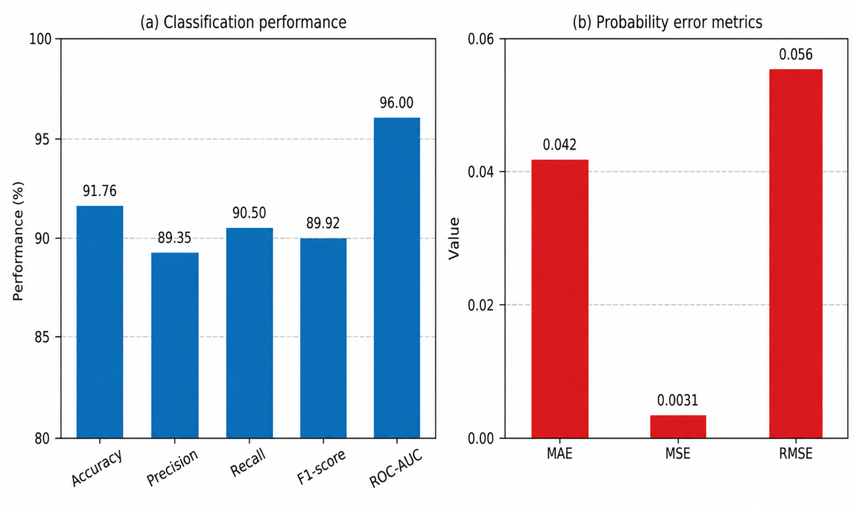
Figure 14: Quantitative performance of GeoPhysML. (a) Classification metrics showing accuracy, precision, recall, F1-score, and ROC–AUC. (b) Probability-based error metrics showing MAE, MSE, and RMSE computed against the observed binary mineralization labels.

3.4 Feature Importance Analysis

In order to understand which geophysical features were important in making the GeoPhysML predictions, we used SHAP (SHapley Additive exPlanations). The mean absolute value of the SHAP was used to rank the importance of features,

Importance(fj)=1n∑i=1n|SHAPi(fj)|,(42)

which represents the average magnitude of the contribution of feature fj across all samples, irrespective of sign.

The feature ranking is shown in Fig. 15. The most important predictor is chargeability (mc), followed by tilt derivative (TDR). Resistivity (ρ) is a secondary predictor, while the first vertical derivative (1VD), reduced to pole (RTP) and total magnetic intensity (TMI) are of minor importance. This hierarchy is in agreement with the mineral system interpretation. The chargeability response is the primary geophysical response to disseminated sulphides, while TDR measures the structural controls on hydrothermal fluid circulation and mineralisation.

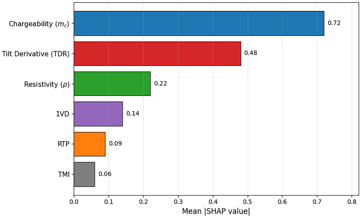
Figure 15: Feature importance ranking based on mean absolute SHAP values. Chargeability (mc) is the dominant predictor, followed by tilt derivative (TDR), resistivity (ρ), 1VD, RTP, and TMI.

The lower ranking of RTP and TMI suggests that amplitude variations are not as indicative as the electrical and structural responses. Overall, the SHAP ranking suggests that GeoPhysML is influenced primarily by the joint occurrence of chargeability anomalies and derivative-based structural attributes, which is consistent with the interpretation that sulphide mineralization in the Maitengwe Greenstone Belt is structurally controlled.

In addition to the ranking of the features, the sign of the SHAP values indicate whether the features tends to increase or decrease the prediction of the model. Mineralization is interpreted as being favoured by increasing chargeability, as borne out by the positive SHAP values, from chargeability associated with disseminated sulphides.

If the SHAP value is positive and near the zero-crossings (TDR≈0), the boundaries are magnetic source boundaries. This observation suggests that the structural contacts, especially the shear zones and fault-controlled boundaries may be favourable fluid pathways for the migration of hydrothermal fluids and later sulphide mineralization.

The model output is more complexly and non-linearly influenced by resistivity. Positive SHAP values are associated with moderate values of resistivity (200–500 Ω⋅m), which are indicative of mineralization favorable conditions. Conversely, very high resistivity values (>1500 Ω⋅m) produce negative SHAP values indicating silicification of the rocks could also reduce rock porosity and permeability, which would limit fluid flow and sulphide deposition. The results show that the GeoPhysML model is able to represent geologically relevant relationships between geophysical characteristics and mineralization processes.

3.5 Ablation Study

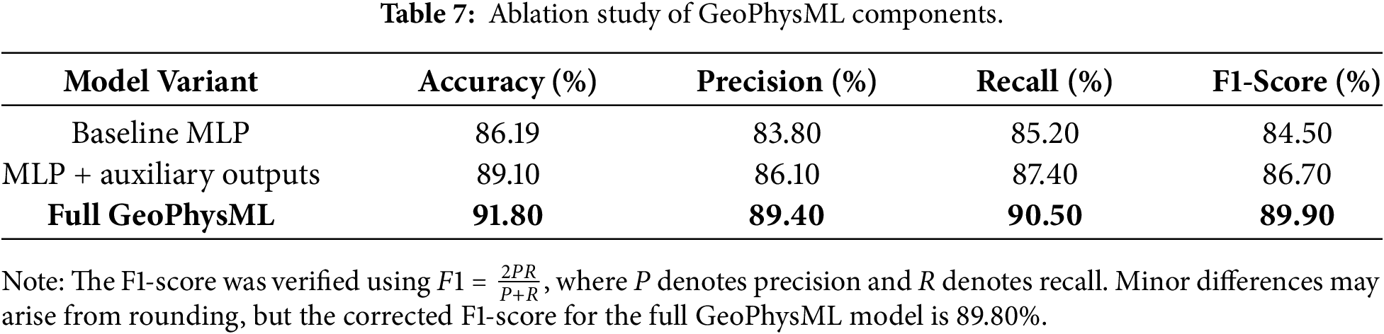
The contribution of the main components of GeoPhysML was evaluated in an ablation study. Three different variants of the model were tested: (i) a baseline MLP that was trained only to classify the mineralization as one of the two classes, (ii) an MLP model with auxiliary outputs of the resistivity and chargeability but without physics-informed loss terms, and (iii) the full GeoPhysML model that combines the auxiliary outputs with the physics-informed loss terms. For all variants, the same set of combined features was used for training, the same train/validation/test split was used for evaluation.

As each component was added, performance improved over time as shown in Table 7. All classification metrics were enhanced when auxiliary resistivity and chargeability outputs were included in the MLP, in comparison to the baseline MLP, indicating that the multi-output formulation helped the network learn a more informative representation of the subsurface. The full GeoPhysML model gave the best results, outperforming the auxiliary-output model in terms of accuracy, precision, recall, and F1 score. This finding indicates that the physics-informed regularization did not just assist with the neural architecture and fused feature set, but also adds value. Combining the ablation results, it is seen that the auxiliary multi-output design and physically constrained optimization contribute to the predictive gain of GeoPhysML and when taken together point to the design of either.

3.6 Comparisons with Baseline Models

The performance of GeoPhysML was evaluated against both geoscience-based and machine-learning baselines to determine whether the proposed framework provides a measurable advantage over conventional interpretation methods and standard predictive models. The geoscience-based baselines comprised a threshold-anomaly approach (mc>8 mV/V, ρ<100 Ω⋅m), a fuzzy weighted-overlay model, and a weights-of-evidence (WoE) model. Machine-learning algorithms used as baselines were logistic regression (LR), support vector machine (SVM), k-nearest neighbour (k-NN), random forest (RF), XGBoost and multilayer perceptron (MLP).

It utilised the same classification metrics for accuracy, precision, recall and F1-score. This comparison sought to determine if the combination of geophysical constraints with empirical supervised learning enhances prediction of mineralization over empirical anomaly mapping, combination of statistical evidence, and traditional machine-learning models. The results are shown in Table 8.

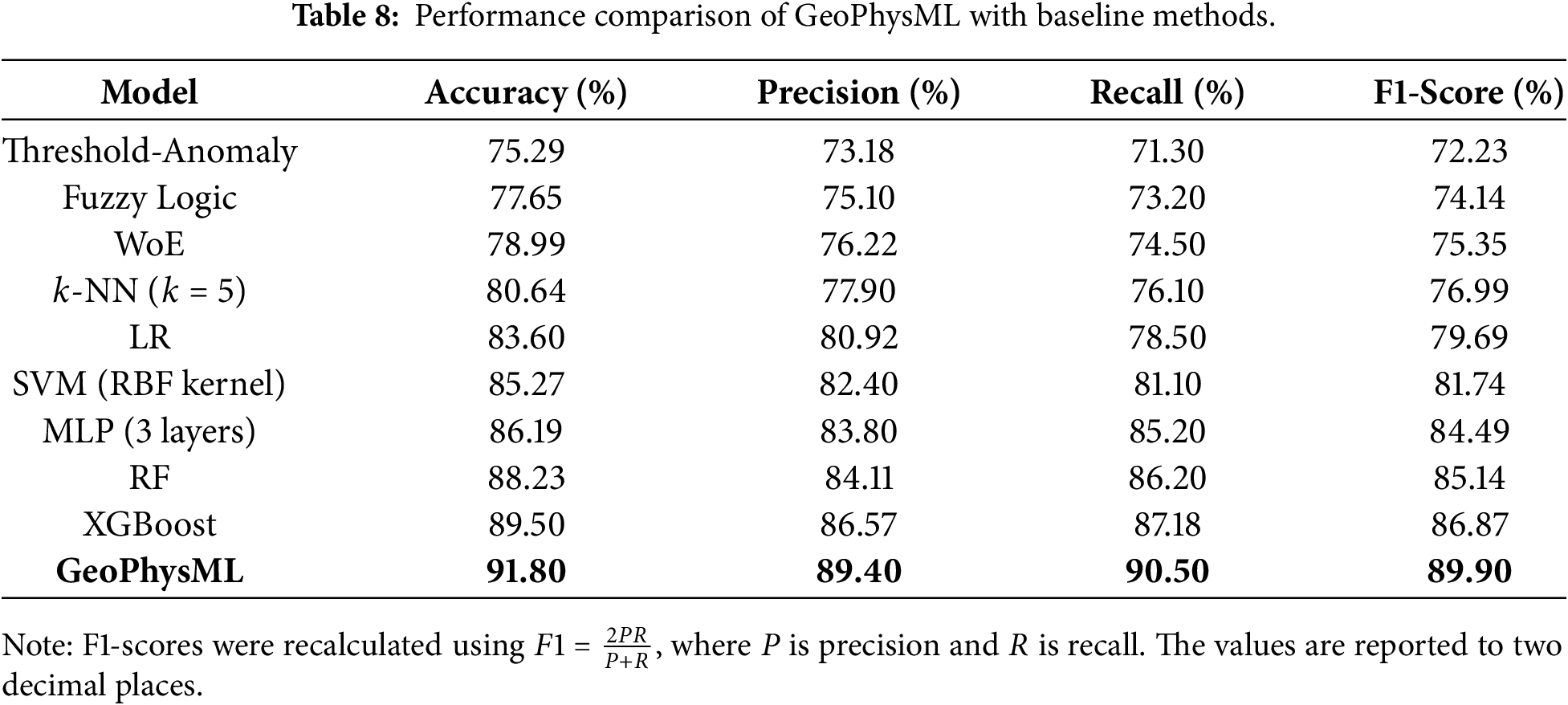
Table 8 shows that GeoPhysML achieved the strongest performance among all evaluated methods, including both geoscience-based and conventional machine-learning baselines. The accuracy values of the geoscience baselines were 75.29%, 77.65%, and 78.99% for the threshold-anomaly, fuzzy logic, and WoE models, respectively, with corrected F1-scores of 72.23%, 74.14%, and 75.35%, respectively. This suggests that empirical anomaly mapping and evidence-combination models capture part of the mineralization pattern, but remain weaker than supervised classifiers.

Among the machine-learning baselines, XGBoost achieved the strongest conventional performance, with 89.50% accuracy, 86.57% precision, 87.18% recall, and a corrected F1-score of 86.87%. GeoPhysML achieved the best overall performance, with 91.80% accuracy, 89.40% precision, 90.50% recall, and a corrected F1-score of 89.90%. Relative to XGBoost, GeoPhysML improved accuracy by 2.60 percentage points, precision by 2.83 percentage points, recall by 3.02 percentage points, and F1-score by 2.93 percentage points. This suggests that the incorporation of geophysical regularization and multi-attribute structure enhanced discrimination between mineralized and non-mineralized areas.

Receiver operating characteristic (ROC) analysis provides a complementary assessment of classifier behaviour across decision thresholds. The corresponding ROC curves and AUC values are shown in Fig. 16.

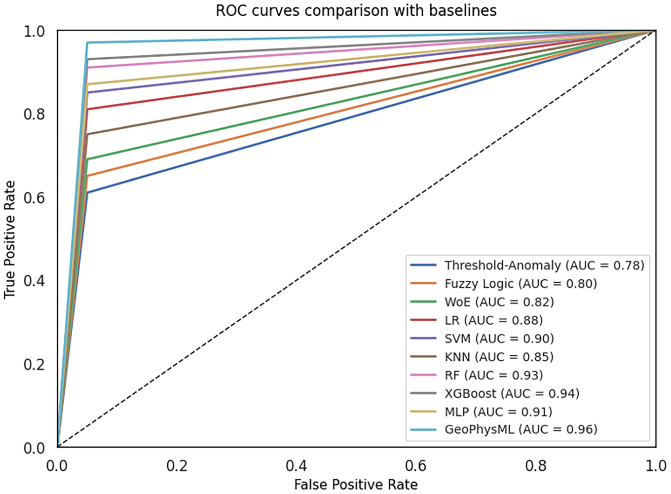
Figure 16: ROC curve comparison of GeoPhysML and the baseline models. GeoPhysML achieves the highest AUC, indicating the strongest discrimination between mineralized and non-mineralized samples across decision thresholds.

Fig. 16 shows that GeoPhysML achieved the highest ROC–AUC value of 0.96, indicating the strongest overall discrimination between mineralized and non-mineralized samples across decision thresholds. Among the baseline models, XGBoost achieved the strongest conventional performance, with 89.50% accuracy, 86.57% precision, 87.18% recall, and a corrected F1-score of 86.87%. GeoPhysML achieved the best overall performance, with 91.80% accuracy, 89.40% precision, 90.50% recall, and a corrected F1-score of 89.90%. Relative to XGBoost, GeoPhysML improved accuracy by 2.60 percentage points and F1-score by 2.93 percentage points as shown in Table 8.

4  Conclusion

4.1 Geological Finding

The integrated geophysical interpretation identified a structurally controlled NE–SW trending target corridor within the Maitengwe Greenstone Belt. Coincident high chargeability values (6.4–10.7 mV/V) and elevated resistivity values (1400–3053 Ω⋅m) characterize altered and silicified amphibolite units containing disseminated pyrite. This geophysical signature is interpreted as indicative of structurally controlled sulphide mineralization rather than barren resistive lithologies.

4.2 Geophysical Finding

IP–ERI inversion delineated three chargeability zones: Zone A (1.8–2.5 mV/V), Zone B (3.4–5.3 mV/V), and Zone C (6.4–10.7 mV/V). Similarly, three resistivity domains were identified: Zone I (15.6–96.1 Ω⋅m), Zone II (180–850 Ω⋅m), and Zone III (1400–3053 Ω⋅m). The deep chargeability anomaly (Zone C) and the deep resistivity anomaly (Zone III) exhibit strong spatial correspondence with the mineralized interval intersected by borehole MTW4 between depths of 118 and 153 m. Furthermore, aeromagnetic derivative analysis revealed NE–SW trending lineaments interpreted as regional shear zones that controlled hydrothermal fluid circulation and sulphide deposition.

4.3 Machine Learning Result

The GeoPhysML framework has an overall classification accuracy of 91.80%, an F1 score of 89.90%, and an ROC-AUC value of 0.96. The classification accuracy of GeoPhysML was 2.60 percentage points higher than the XGBoost benchmark model and the F1-score was improved by 2.93 percentage points. The most influential predictive variables were determined via interpretability analysis using SHAP. Additionally, the uncertainty quantification with Monte Carlo dropout (100 forward passes) found that the most important target zone had a relatively low uncertainty, with the uncertainty index (UI) <0.15, which boosted the confidence in the model predictions.

4.4 Limitations

There are a number of limitations which need to be recognized, but the results are encouraging. First, the model validation relied on borehole MTW4, which was held out from training for independent assessment. The training labels were derived from MTW1 (110–160 m) and MTW2 (118–153 m), which contain disseminated sulphide mineralization with ≥5% pyrite and quartz-carbonate veining. MTW3 did not intersect significant sulphides and was used as a negative sample. Secondly, the size of the labelled dataset is relatively small (247 grid cells) and the performance metrics of the models may still be optimistic even after implementing spatial blocking. Thirdly, the pseudo-3D reconstruction produced with the IP-ERI data suffers from low cross-line resolution as a result of a survey line spacing of 100 m. Lastly, the identified sulphide-bearing zones are regarded as sub-economic and typically comprise pyrite with lesser chalcopyrite, and with less than 0.1% of base metals content and hence are not currently regarded as ore grade mineralisation.

4.5 Future Scope

Independent drilling programs in the future to test the high probability targets that GeoPhysML has predicted outside of the immediate area of borehole MTW4 is a suggested area for further work. Further borehole geochemistry such as X-ray diffraction (XRD) and whole rock geochemistry assays would give better constraints on alteration characteristics and sulphide mineralogy. Furthermore, application of the GeoPhysML framework to other greenstone belts, such as the Tati and Matsitama Greenstone Belts, would provide a robust assessment of the model’s transferability and general applicability for mineral exploration.

Acknowledgement: Not applicable.

Funding Statement: The authors received no specific funding for this study.

Author Contributions: Vae Onalethata led the study, data analysis, geological interpretation, and manuscript drafting. Boniface Kgosidintsi, Bokani Nthaba, and Elisha M. Shemang contributed to geophysical interpretation and manuscript review. Abid Yahya contributed to the machine-learning framework, mathematical formulation, and technical revision. Mohamed Yasin Abdul Salam, Yar Muhammad, Enerst Edozie, and Asiimwe Eva contributed to technical review, validation, and final manuscript refinement. All authors reviewed and approved the final manuscript.

Availability of Data and Materials: The generated dataset used in this study is publicly available on GitHub at https://github.com/Mdnyasin/geogly.git.

Ethics Approval: Not applicable.

Conflicts of Interest: The authors declare no conflicts of interest.

References

1. Kwan K, Johnson I, Legault JM, Khaled K, Prikhodko A. Understanding Archean greenstone-hosted lode gold mineralization in Ontario, Canada through helicopter TDEM data. Explor Geophys. 2019;50(6):1–4. doi:10.1080/22020586.2019.12072985. [Google Scholar] [CrossRef]

2. Chen X, Liu J. Enrichment of iron ores by folding in the BIF-hosted deposit: a case study from the Archean Qian’an iron deposit, North China Craton. Geol J. 2018;53(2):617–28. doi:10.1002/gj.2916. [Google Scholar] [CrossRef]

3. Fayol N, Jébrak M. Archean sanukitoid gold porphyry deposits: a new understanding and genetic model from the Lac Bachelor gold deposit, Abitibi, Canada. Econ Geol. 2017;112(8):1913–36. doi:10.5382/econgeo.2017.4534. [Google Scholar] [CrossRef]

4. Filipa A, Marques A, Barriga FJAS, Scott SD. Sulfide mineralization in an ultramafic-rock hosted seafloor hydrothermal system: from serpentinization to the formation of Cu–Zn–(Co)-rich massive sulfides. Mar Geol. 2007;245(1–4):20–39. doi:10.1016/j.margeo.2007.05.007. [Google Scholar] [CrossRef]

5. Aldiss DT. The motloutse complex and the Zimbabwe craton/limpopo belt transition in Botswana. Precambrian Res. 1991;50(1–2):89–109. doi:10.1016/0301-9268(91)90049-G. [Google Scholar] [CrossRef]

6. McCourt S, Kampunzu AB, Bagai Z, Armstrong RA. The crustal architecture of Archaean terranes in Northeastern Botswana. South Afr J Geol. 2004;107(1–2):147–58. doi:10.2113/107.1-2.147. [Google Scholar] [CrossRef]

7. Key RM. The evolution of the archaean crust of northeast Botswana. Precambrian Res. 1976;3(4):375–413. doi:10.1016/0301-9268(76)90028-0. [Google Scholar] [CrossRef]

8. Maier WD, Barnes SJ, Chinyepi G, Barton JM, Eglington B, Setshedi I. The composition of magmatic Ni-Cu-(PGE) sulfide deposits in the Tati and Selebi-Phikwe belts of eastern Botswana. Miner Depos. 2008;43(1):37–60. doi:10.1007/s00126-007-0143-5. [Google Scholar] [CrossRef]

9. Hofmann A, Bekker A. Comparing orthomagmatic and hydrothermal mineralization models for komatiite-hosted nickel deposits in Zimbabwe using multiple-sulfur, iron, and nickel isotope data. Miner Depos. 2014;49(1):75–100. doi:10.1007/s00126-013-0476-1. [Google Scholar] [CrossRef]

10. Harris J, Strong J, Thurston P, Nymoen K, Haugaard R, Naghizadeh M, et al. Mineral prospectivity mapping and differential metal endowment between two greenstone belts in the Canadian Superior Craton: JR Harris et al. Nat Resour Res. 2025;34(1):97–120. doi:10.1007/s11053-024-10432-3. [Google Scholar] [CrossRef]

11. Li Y, Alkhalifah T, Zhang Z. Deep-learning assisted regularized elastic full waveform inversion using the velocity distribution information from wells. Geophys J Int. 2021;226(2):1322–35. doi:10.1093/gji/ggab162. [Google Scholar] [CrossRef]

12. Wang Z, Zuo R. Intelligent lithological mapping: challenges and future prospective: Wang and Zuo. Nat Resour Res. 2026;35(1):279–312. [Google Scholar]

13. El-Omairi MA, El Garouani A, Abdellatif M, El Garouani M, Boumehdi M, Shebl A. Remote sensing and aeromagnetic data integration for mapping Cu, Mn, Co, Ba, and Fe mineralization: a case study from Aït Semgane, Anti-Atlas, Morocco. Ore Geol Rev. 2025;183(6):106701. doi:10.1016/j.oregeorev.2025.106701. [Google Scholar] [CrossRef]

14. El-Omairi MA, El Garouani M, El Garouani A. Enhanced lithological mapping via remote sensing: employing SVM, random trees, ANN, with MNF and PCA transformations. Egypt J Remote Sens Space Sci. 2025;28:34–52. [Google Scholar]

15. Puzyrev V. Deep learning electromagnetic inversion with convolutional neural networks. Geophys J Int. 2019;218(2):817–32. doi:10.1093/gji/ggz204. [Google Scholar] [CrossRef]

16. Nidhi DK, Chaudhary J, Heikkonen J, Kanth R. Enhancing mineral prospectivity mapping with contrastive representation learning and dimensionality reduction techniques. In: Ali M, Verma AK, Verma OP, Edeh MO, Rajpurohit J, editors. Hybrid intelligence: theories and applications. Singapore: Springer; 2026. p. 13–23. [Google Scholar]

17. Thawon I, Vo D, Bui TQ, Rattanamongkhonkun K, Chamroon C, Tippayawong N, et al. Physics-informed neural networks: current progress and challenges in computational solid and structural mechanics. Comp Model Eng. 2026;146(2):2. doi:10.32604/cmes.2026.077044. [Google Scholar] [CrossRef]

18. Van Waarden C. Prehistoric copper mining in Botswana. In: Selin H, editor. Encyclopaedia of the history of science, technology, and medicine in non-western cultures. Dordrecht, The Netherlands: Springer; 2014. p. 1–13. doi:10.1007/978-94-007-3934-5_9871-1. [Google Scholar] [CrossRef]

19. Abu El-Ata AS, El-Khafeef AA, Ghoneimi AE, Abd Alnabi SH, Al-Badani MA. Applications of aeromagnetic data to detect the Basement Tectonics of Eastern Yemen region. Egypt J Pet. 2013;22(2):277–92. doi:10.1016/j.ejpe.2013.06.007. [Google Scholar] [CrossRef]

20. Al-Ibiari MG, Ismail AAM, El-Khafeef AA, Basheer AA, El-laban AMM, Tarek Y. Analysis and interpretation of aeromagnetic data for Wadi Zeidun area, Central Eastern Desert, Egypt. Egypt J Pet. 2018;27(3):285–93. doi:10.1016/j.ejpe.2017.04.002. [Google Scholar] [CrossRef]

21. Anand SP, Rajaram M. Aeromagnetic data analysis for the identification of concealed uranium deposits: a case history from Singhbhum uranium province, India. Earth Planets Space. 2006;58(8):1099–103. doi:10.1186/BF03352616. [Google Scholar] [CrossRef]

22. Leseane K, Betts P, Armit R, Ailleres L. Structural overprinting criteria determined from regional aeromagnetic data: an example from the Hill End Trough, East Gondwana. Tectonophysics. 2020;797(1):228660. doi:10.1016/j.tecto.2020.228660. [Google Scholar] [CrossRef]

23. Robertson DJ, Vidanovich PNP, Zoellner SK, Meyers JB. Interpretation of aeromagnetic data in the Franklin area, northern New Zealand. N Z J Geol Geop. 2017;60(1):36–50. doi:10.1080/00288306.2016.1256328. [Google Scholar] [CrossRef]

24. Rodríguez JAB, Carmenates Y, González JDM. Interpretation of aeromagnetic data using GIS to evaluate the geotectonic regime of the Sabinas Basin. Earth Sci Res J. 2017;21(4):175–81. doi:10.15446/esrj.v21n4.57924. [Google Scholar] [CrossRef]

25. Salem A, Ali MY. Mapping basement structures in the northwestern offshore of Abu Dhabi from high-resolution aeromagnetic data. Geophys Prospect. 2016;64(3):726–40. doi:10.1111/1365-2478.12266. [Google Scholar] [CrossRef]

26. Revil A, Vaudelet P, Su Z, Chen R. Induced polarization as a tool to assess mineral deposits: a review. Minerals. 2022;12(5):571. doi:10.3390/min12050571. [Google Scholar] [CrossRef]

27. Dusabemariya C, Qian W, Bagaragaza R, Faruwa AR, Ali M. Some experiences of resistivity and induced polarization methods on the exploration of sulfide: a review. J Geosci Environ Prot. 2020;8(11):68–92. doi:10.4236/gep.2020.811004. [Google Scholar] [CrossRef]

28. Zhou B, Khalil I. Electrical resistivity tomography: a subsurface-imaging technique. In: Applied geophysics with case studies on environmental, exploration and engineering geophysics. London, UK: IntechOpen; 2018. p. 1–16. doi:10.5772/intechopen.81511. [Google Scholar] [CrossRef]

29. Loke MH, Chambers JE, Rucker DF, Kuras O, Wilkinson PB. Recent developments in the direct-current geoelectrical imaging method. J Appl Geophys. 2013;95(4):135–56. doi:10.1016/j.jappgeo.2013.02.017. [Google Scholar] [CrossRef]

30. Aster RC, Borchers B, Thurber CH. Parameter estimation and inverse problems. 3rd ed. Amsterdam, The Netherlands: Elsevier; 2018. [Google Scholar]

31. Litherlands M. Geology of Maitengwe area. Lobatse: Geological Surveys Department; 1975. doi:10.14509/15287. [Google Scholar] [CrossRef]

32. Holmes H, Gledhill P, Chatupa J, Akanyang P. Geophysics in the Maitengwe greenstone belt. In: Proceedings of the 3rd SAGA Biennial Conference and Exhibition. European Association of Geoscientists & Engineers; 1993 Apr 14–16; Cape Town, South Africa. p. cp-224. doi:10.3997/2214-4609-pdb.224.048. [Google Scholar] [CrossRef]

33. Smith RA. The lithostratigraphy of the Karoo Supergroup in Botswana. A report on the geophysical and geological results of follow-up drilling to the Aeromagnetic Survey of Botswana. Geol Mag. 1986;123(6):710–1. doi:10.1017/s0016756800024328. [Google Scholar] [CrossRef]

34. Chukwu C, Betts P, Moore D, Munukutla R, Armit R, McLean M, et al. Unsupervised machine learning and depth clusters of Euler deconvolution of magnetic data: a new approach to imaging geological structures. Explor Geophys. 2024;55(3):223–45. doi:10.1080/08123985.2023.2299475. [Google Scholar] [CrossRef]

35. Subasinghe ND, Charles WKDGDR, De Silva SN. Analytical signal and reduction to pole interpretation of total magnetic field data at Eppawala phosphate deposit. J Geosci Environ Prot. 2014;2(3):181–9. doi:10.4236/gep.2014.23023. [Google Scholar] [CrossRef]

36. Ansari A, Alamdar K. A new edge detection method based on the analytic signal of tilt angle (ASTA) for magnetic and gravity anomalies. Iran J Sci. 2011;35(2):81–8. doi:10.1190/ist092012-001.75. [Google Scholar] [CrossRef]

37. Blakely RJ. Potential theory in gravity and magnetic applications. Cambridge, UK: Cambridge University Press; 1996. [Google Scholar]

38. Pal SK, Vaish J, Kumar S, Priyam P. Downward continuation and tilt derivative of magnetic data for delineation of concealed coal fire in East Basuria Colliery, Jharia coal field, India. J Earth Sys Sci. 2017;126(4):53. doi:10.1007/s12040-017-0826-y. [Google Scholar] [CrossRef]

39. Mousa A, Al-Rahim A. Lineaments determination of Western part of Iraqi western desert using aeromagnetic and gravity data. Aust J Basic Appl Sci. 2016;2(12):321. [Google Scholar]

40. Abdelrahman K, Pham LT, Oliveira SP, Duong VH, Duy TK, Gomez-Ortiz D, et al. Reliable tilt-depth estimates based on the stable computation of the tilt angle using robust vertical derivatives. Sci Rep. 2024;14(1):7392. doi:10.1038/s41598-024-57314-5. [Google Scholar] [CrossRef]

41. Mogotsi IC, Mannathoko IZ. Spatial data management for water resource management: the Botswana wellfield monitoring program. Inf Dev. 2001;17(3):147–54. doi:10.1177/0266666014240890. [Google Scholar] [CrossRef]

42. Okpoli CC. Sensitivity and resolution capacity of electrode configurations. Int J Geophys. 2013;2013(1):608037. doi:10.1155/2013/608037. [Google Scholar] [CrossRef]

43. Reynolds JM. An introduction to applied and environmental geophysics. Hoboken, NJ, USA: John Wiley & Sons; 2011. [Google Scholar]

44. Sumner JS. Principles of induced polarization for geophysical exploration. In: Developments in economic geology. Vol. 5. Amsterdam, The Netherlands: Elsevier; 2012. [Google Scholar]

45. Dahlin T. Short note on electrode charge-up effects in DC resistivity data acquisition using multi-electrode arrays. Geophys Prospect. 2000;48(1):181–7. doi:10.1046/j.1365-2478.2000.00172.x. [Google Scholar] [CrossRef]

46. He Z, Cai H, Li S, Xian J, Hu X. Extracting IP parameters of rock samples using machine learning. Geophys J Int. 2023;235(1):862–78. doi:10.1093/gji/ggad288. [Google Scholar] [CrossRef]

47. Ali M, Sun S, Qian W, Bohari AD, Claire D, Faruwa AR, et al. Borehole resistivity and induced polarization tomography at the Canadian shield for mineral exploration in north-western Sudbury. E3S Web Conf. 2020;168:00002. doi:10.1051/e3sconf/202016800002. [Google Scholar] [CrossRef]

48. Martínez J, Rey J, Sandoval S, Hidalgo MC, Mendoza R. Geophysical prospecting using ERT and IP techniques to locate Galena veins. Remote Sens. 2019;11(24):2923. doi:10.3390/rs11242923. [Google Scholar] [CrossRef]

49. Kearey P, Brooks M, Hill I. An introduction to geophysical exploration. 3rd ed. Oxford, UK: Blackwell Science Ltd.; 2002. doi:10.1017/s0016756803378021. [Google Scholar] [CrossRef]

50. Dahlin T, Leroux V. Improvement in time-domain induced polarization data quality with multi-electrode systems by separating current and potential cables. Near Surf Geophys. 2012;10(6):545–65. doi:10.3997/1873-0604.2012028. [Google Scholar] [CrossRef]

51. Loke MH, Barker RD. Rapid least-squares inversion of apparent resistivity pseudosections by a quasi-Newton method. Geophys Prospect. 1996;44(1):131–52. doi:10.3997/2214-4609.201409781. [Google Scholar] [CrossRef]

52. Gribenko A, Zhdanov M. Regularized Gauss-Newton method of nonlinear geophysical inversion in the data space: applications to 3D magnetotelluric inversion. In: 2017 SEG International Exposition and Annual Meeting. Houston, TX, USA: Society of Exploration Geophysicists; 2017. p. 1126–30. [Google Scholar]

53. Loke MH, Acworth I, Dahlin T. A comparison of smooth and blocky inversion methods in 2D electrical imaging surveys. Explor Geophys. 2003;34(3):182–7. doi:10.1071/EG03182. [Google Scholar] [CrossRef]

54. Rucker C, Erickson BA. Physics-informed deep learning of rate-and-state fault friction. Comput Methods Appl Mech Eng. 2024;430(7140):117211. doi:10.1016/j.cma.2024.117211. [Google Scholar] [CrossRef]

55. Goodfellow I, Bengio Y, Courville A, Bengio Y. Deep learning. Vol. 1. Cambridge, MA, USA: MIT Press Cambridge; 2016. doi:10.1007/s10710-017-9314-z. [Google Scholar] [CrossRef]

56. Shim JW. Enhancing cross entropy with a linearly adaptive loss function for optimized classification performance. Sci Rep. 2024;14(1):27405. doi:10.1038/s41598-024-78858-6. [Google Scholar] [CrossRef]

57. Schuster GT, Chen Y, Feng S. Review of physics-informed machine-learning inversion of geophysical data. Geophysics. 2024;89(6):T337–56. doi:10.1190/geo2023-0615.1. [Google Scholar] [CrossRef]

58. Raissi M, Perdikaris P, Karniadakis GE. Physics-informed neural networks: a deep learning framework for solving forward and inverse problems involving nonlinear partial differential equations. J Comput Phys. 2019;378:686–707. [Google Scholar]

59. Salam MYA, Ogunmuyiwa EN, Manisa VK, Yahya A, Badruddin IA. Microstructural characterization and hardness prediction of AlCuCrFeNi high entropy alloys using transformer-based physics-informed neural networks (T-PINN). J Mater Res Technol. 2025;38:1934–46. doi:10.1016/j.jmrt.2025.08.021. [Google Scholar] [CrossRef]

60. Karniadakis GE, Kevrekidis IG, Lu L, Perdikaris P, Wang S, Yang L. Physics-informed machine learning. Nat Rev Phys. 2021;3(6):422–40. doi:10.1038/s42254-021-00314-5. [Google Scholar] [CrossRef]

61. Modoranu IV, Safaryan M, Malinovsky G, Kurtic E, Robert T, Richtárik P, et al. MicroAdam: accurate adaptive optimization with low space overhead and provable convergence. Adv Neural Inf Process Syst. 2024;37:1–43. [Google Scholar]

62. Braguta VV, Chernodub MN, Roenko AA, Sychev DA. Negative moment of inertia and rotational instability of gluon plasma. Phys Lett B. 2024;852(3):138604. doi:10.1016/j.physletb.2024.138604. [Google Scholar] [CrossRef]

63. Yi MJ, Kim JH, Song Y, Cho SJ, Chung SH, Suh JH. Three-dimensional imaging of subsurface structures using resistivity data. Geophys Prospect. 2001;49(4):483–97. doi:10.1046/j.1365-2478.2001.00269.x. [Google Scholar] [CrossRef]

64. Sono P, Nthaba B, Shemang EM, Kgosidintsi B, Seane T. An integrated use of induced polarization and electrical resistivity imaging methods to delineate zones of potential gold mineralization in the Phitshane Molopo area, Southeast Botswana. J Afr Earth Sci. 2021;174:104060. doi:10.1016/j.jafrearsci.2020.104060. [Google Scholar] [CrossRef]

65. Goldie M. Self-potentials associated with the Yanacocha high-sulfidation gold deposit in Peru. Geophysics. 2002;67(3):684–9. doi:10.1190/1.1484511. [Google Scholar] [CrossRef]

66. Dakir I, Benamara A, Aassoumi H, Ouallali A, Ait Bahammou Y. Application of induced polarization and resistivity to the determination of the location of metalliferous veins in the Taroucht and Tabesbaste areas (Eastern Anti-Atlas, Morocco). Int J Geophys. 2019;2019(1):5849019. doi:10.1155/2019/5849019. [Google Scholar] [CrossRef]

67. Antonelli F, Stevanato R, Fries M, Abreu G, Ferreira FJF, Serrano V. Resistivity and induced polarization applied to epithermal gold deposit in the Torre Target, at Castro Basin-PR. In: Proceedings of the 16th International Congress of the Brazilian Geophysical Society; 2019 Aug 19–22; Rio de Janeiro, Brazil. p. 1–5. [Google Scholar]

68. Mashhadi S, Ramazi H. The application of resistivity and induced polarization methods in identification of skarn alteration haloes: a case study in the Qale-Alimoradkhan Area. J Environ Eng Geophys. 2018;23(3):363–8. doi:10.2113/jeeg23.3.363. [Google Scholar] [CrossRef]

69. Kendall A, Gal Y. What uncertainties do we need in Bayesian deep learning for computer vision? Adv Neural Inf Process Syst. 2017;30:5580–90. [Google Scholar]