Topological Optimisation Design of Nanofluid-Cooled Microchannel Heat Sink Using a Three-Layer Thermofluid Model for Electronics Cooling

1  Introduction

With the sustained promotion of electronic equipment in the pursuit of greater efficiency and more compact structural design, thermal management has become increasingly essential to the performance and reliability of modern electronic packaging systems [1,2]. As an effective solution for thermal management, microchannel heat sinks (MCHS) have gained widespread adoption in electronic cooling applications [3]. In such systems, heat generated by the chip is transferred through the metal substrate via conduction into the microchannels of the MCHS. The coolant flowing through these channels then removes it via convective heat transfer. Consequently, both the flow channel geometry and the choice of coolant significantly influence the overall thermal performance of MCHS.

The heat transfer performance of MCHS can be effectively enhanced through the optimization of their geometric configurations. Currently, the mainstream optimization approaches for MCHS primarily encompass size optimization and shape optimization. Representative methods under these two categories include the conjugate gradient method [4,5], particle swarm optimization [6,7], and genetic algorithms [8], to name a few. However, these conventional optimization methods are inherently constrained by predefined geometric frameworks, which leads to limited design freedom and imposes significant restrictions on the comprehensive optimization of flow channel structures.

As a structural optimization method, topological optimisation [9] does not rely on a predefined initial structure and allows for simultaneous changes in size, shape, and topology. This provides greater design freedom and enables significant improvements in structural performance. Topological optimisation originated in the field of solid mechanics [10,11] and has since been widely applied in various physical disciplines [12,13], including optics, acoustics, electromagnetics, fluid mechanics [14–17], and heat transfer [18–22]. Currently, the prevailing topological optimisation techniques cover the homogenization method, the density method, the level set approach, as well as the evolutionary structural optimization method [13]. The application of topological optimisation to fluid dynamics dates back to Borrvall and Petersson’s groundbreaking study in 2003 [14], which initiated the use of topological optimisation for Stokes flow fields and established the fundamental theoretical framework based on the density method. Subsequently, a density-based topological optimisation approach for flow problems governed by the Navier–Stokes equations was proposed by Gersborg-Hansen et al. [23]. For unsteady fluid flow, density-based topological optimisation methods were independently developed by Kreissl et al. [16] and Deng et al. [17]. Duan et al. [15,24] and Zhou and Li [25] put forward level set-based topological optimisation methods for Navier-Stokes flows. Additionally, Deng et al. [26] developed a level set method for fluid topological optimisation with body forces considered. Pingen and Maute [27] applied the density method to tackle topological optimisation for non-Newtonian fluid flow problems.

The pioneering work of Dede [18] and Yoon [19] marks the starting point for research on topological optimisation of thermofluid systems; these authors first proposed density-based topological optimisation methods for forced heat transfer scenarios. In their studies, the governing equations adopt a coupled form of the convection-diffusion equation together with the Navier-Stokes equations. Thereafter, Matsumori et al. [28] employed the density-based topological optimisation approach to investigate the design optimization of MCHS under constant inlet power. Koga et al. [29] examined the topological design optimization of microchannel heat sinks with the density method, using a weighted function of flow energy dissipation and heat transfer as the cost function. Zhang et al. [30] performed topological optimisation of nanofluid-cooled heat sinks and assessed how temperature-sensitive fluid properties influence the optimized designs. Alexandersen et al. [31] put forward a density-based topological optimisation method for creating natural-convection cooling structures within a large-scale three-dimensional heat sink. Recently, a multi-scale topological optimisation approach incorporating diverse lattice configurations was proposed by Zhang et al. [32], which is applied to the design of hybrid porous heat sinks for high-power electronic devices.

Although topological optimisation has made significant progress in addressing convective heat transfer problems, several challenging issues persist. Topological optimisation based on a fully three-dimensional thermofluid model requires solving a large number of physical degrees of freedom and typically involves hundreds of iterations, resulting in high computational costs. In contrast, the classical two-dimensional thermofluid model offers lower computational demands; however, it neglects the thermal flow influences in the thickness direction, which leads to considerable errors. McConnell and Pingen [33] pioneered a two-layer thermofluid model and implemented topological optimisation for two-layer heat sinks based on the lattice Boltzmann method. In their study, the 3D MCHS was defined as a bilayer structure composed of a bottom substrate layer and a thermofluid channel layer. Different from conventional two-dimensional (2D) thermofluid models, this approach takes into account the heat exchange between the bottom plate and thermofluid channel, thereby improving the prediction accuracy of temperature fields. Haertel et al. [34] assumed a fixed interlayer heat transfer coefficient to obtain heat flux values and established a two-layer thermofluid topological optimisation model. Similar assumptions have been widely employed in successive studies to build multilayer models for topological optimisation [35–39]. Yan et al. [40] introduced a two-layer heat sink model using the variational dimension reduction method, which is based on invariant temperature profiles along the thickness direction of the thermofluid layer and the substrate. However, this model did not consider the heat-transfer phenomena taking place in the cover plate. Conversely, Zhao et al. [41] devised a three-layer heat transfer model based on the premise of an adaptive temperature distribution over the thickness of the thermofluid channel. Jia et al. [42] proposed a novel three-layer thermofluid model dedicated to power-law fluids and afterwards explored the topological optimisation of microfluidic heat sinks with the use of non-Newtonian fluids.

In addition to optimizing geometric structures, altering coolants also contributes to improving the heat transfer performance of heat sinks. Nanofluids have gained widespread attention due to their high thermal conductivity, which enables performance enhancement of heat sinks [43]. Numerous numerical [44–47] and experimental [48,49] investigations have demonstrated the prominent performance advantages of nanofluid microchannel heat sinks (NCMHS) in thermal management fields. Currently, research on topological optimisation of NCMHS remains relatively scarce. Zhang et al. [30] conducted topological optimisation for NCMHS based on a classical 2D thermofluid model that considers temperature-sensitive thermophysical properties of nanofluids. The study showed that temperature-sensitive fluid properties can significantly impact the optimized designs. Chen and Yaji [50] studied the topological optimisation of NCMHS using an Eulerian-Eulerian approach.

Nanofluids are essentially two-phase mixture systems composed of a continuous base fluid phase and a discrete nanoparticle phase. However, at low nanoparticle volume fractions, due to the nanoscale size of the particles, nanofluids can be approximately regarded as a uniform fluid. Therefore, many researchers [5,30] have adopted a single-phase fluid model in simulating their flow and heat exchange. For this single-phase approach, the nanofluid’s thermophysical properties can be obtained equivalently by using those of the base fluid and the nanoparticles. Considering this, the current work also employs a single-phase nanofluid thermofluid model for describing the convective heat transfer within the NCMHS.

In this study, we utilize a computationally cost-effective multi-layer modeling approach to conduct three-layer topological optimisation of NCMHS, with full consideration of the temperature-sensitive thermophysical properties of the working fluid. By introducing the velocity profile assumption and adaptive temperature profile assumption along the thickness direction, and incorporating the interlayer coupled heat flux derived from Fourier’s law, a three-layer thermofluid model for NCMHS is established. Built upon this model, a three-layer topological optimisation framework for NCMHS is further developed, where the channel layout is represented by a fictitious density field. Moreover, the influences of temperature-sensitive fluid properties and the nanofluid’s characteristics on the optimized channel geometries of the three-layer NCMHS are explored.

It should be emphasized that, compared with the study reported in Reference [30], although both works were devoted to the topological optimisation of the NCMHS, the underlying methodological frameworks are fundamentally distinct. Reference [30] employed a classical two-dimensional thermofluid model that, despite its merits of concise formulation and low computational cost, neglected the heat conduction in the bottom and top plates as well as the effects of solid walls and heat transfer in the thickness direction on the thermofluid layer, resulting in significant deviations from actual physical scenarios. In contrast, the three-layer thermofluid model developed in this study fully accounts for the aforementioned factors, thereby enabling a more accurate characterization of the flow and heat transfer behaviors within the NCMHS.

2  Physical Model

2.1 Geometric Model

As shown in Fig. 1, the NCMHS adopts a three-layer structure, which comprises a base plate, thermo-fluid channel, and top plate. For the top surface of the upper plate, an adiabatic boundary condition is adopted, while the chip serves as the heat source and is tightly bonded to the base plate. Heat first conducts inside the base plate and is transmitted to the internal cooling channel of the NCMHS. The circulating coolant then flows through the channel and dissipates heat by means of convective heat transfer.

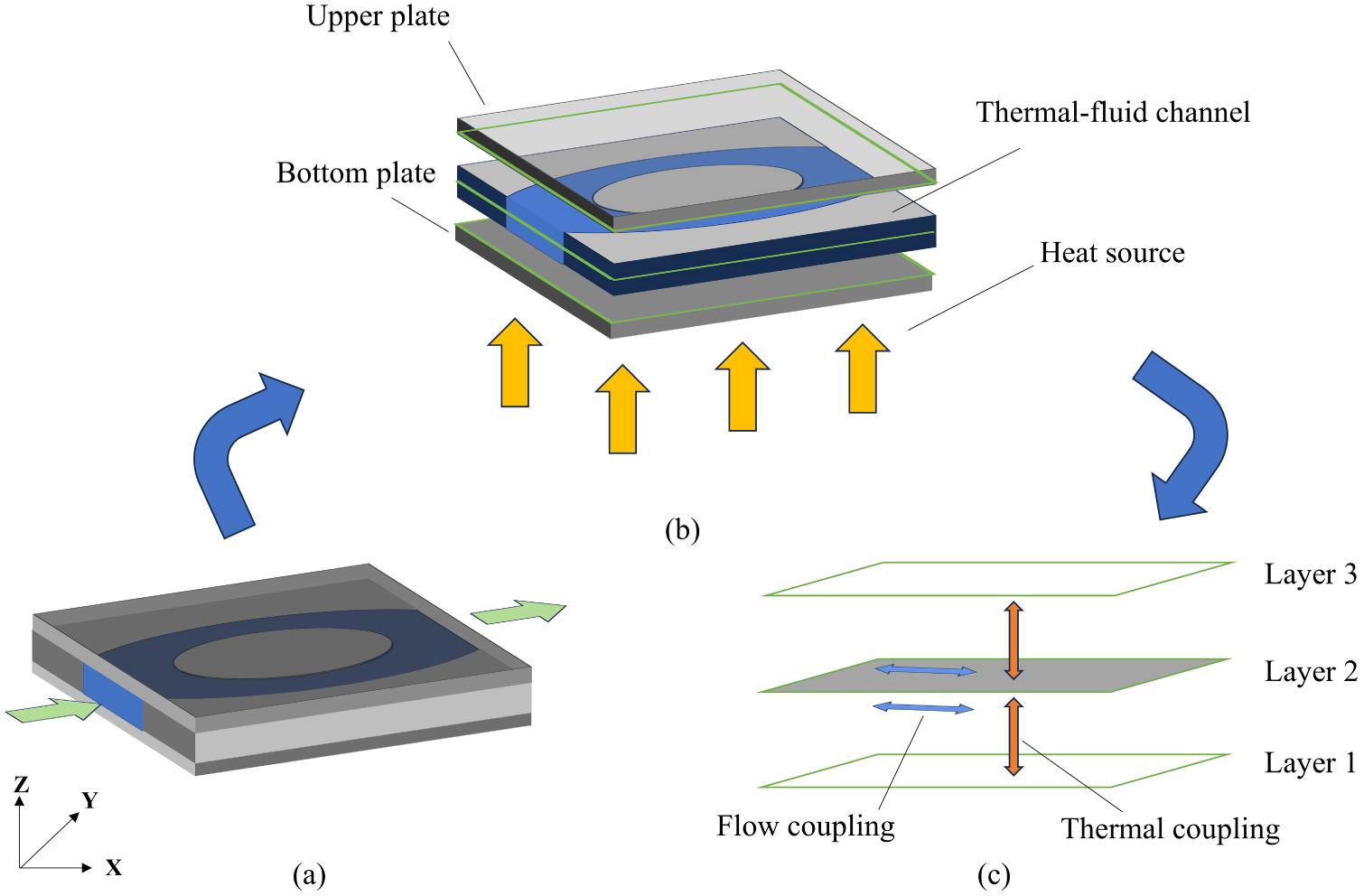
Figure 1: Schematic diagram of nanofluid-cooled microchannel heat sinks used in this paper: (a) 3D view, (b) three-layer geometric structure, and (c) three-layer thermofluid coupling model.

Layer 1 and Layer 3 represent the bottom and upper plates, respectively. As the contact surface between the bottom plate and the thermal fluid channel serves as a critical reference plane for heat transfer analysis, Layer 1 is specified at this exact location. By the same token, Layer 3 is defined on the interface between the top plate and the thermal fluid channel. Layer 2 refers to the thermofluid channel, which is specifically defined as the central cross-section of the channel. The thickness values of the two cover plates and the thermofluid channel are assigned as 0.1 and 0.2 mm correspondingly. The origin of the Cartesian coordinate system is placed on Layer 1, and the z-direction coordinates for Layers 1 to 3 are marked as z1, z2 and z3. The fluid flow governing equations are solved within Layer 2, while the thermal analysis covers both the in-layer heat conduction inside each individual layer and the interfacial thermal coupling between neighboring layers.

2.2 Thermophysical Properties of the Nanofluid

In this study, the Al2O3-H2O nanofluid is approximated as a single-phase fluid with the temperature-sensitive property adopted from [51]. The nanofluid’s dynamic viscosity μnf, specific heat capacity cp,nf, thermal conductivity knf, and density ρnf are defined by

ρnf=(1−ϕp)ρbf+ϕpρp,(1)

cp,nf=(1−ϕp)ρbfcp,bf+ϕpρpcp,pρnf,(2)

μnf×103=−0.4491+28.837TC+0.574ϕp−0.1634ϕp2+23.053ϕp2TC2+0.0132ϕp3−2354.735ϕpTC3+23.498ϕp2dp2−3.0185ϕp3dp2,(3)

knfkbf=0.9843+0.398ϕp0.7383(1dp(nm))0.2246(μnfμbf)0.0235,−3.9517ϕpTC+34.034ϕp2TC3+32.509ϕpTC2(4)

where cp,p = 765 J/(kg∙K) represents the specific heat capacity of Al2O3 nanoparticles and ρp = 3970 kg/m3 represents the density of Al2O3 nanoparticles. The dynamic viscosity (μbf), specific heat capacity (cp,bf), thermal conductivity (kbf), and density (ρbf) of the base fluid are defined as

ρbf=999.79684+0.068317355TC−0.010740248TC2+0.00082140905TC2.5−2.3030988×10−5TC3,(5)

cp,bf=1000×(4.2174356−0.0056181625TC+0.0012992528TC1.5−0.00011535353TC2+4.14964×10−6TC2.5),(6)

μbf=1/(557.82468+19.408782TC+0.1360459TC2−3.1160832×10−4TC3),(7)

kbf=0.5650285+0.0026363895TC−0.00012516934TC1.5−1.5154918×10−6TC2−0.0009412945TC0.5(8)

where TC = (T2 − 273.15)°C represents the temperature in Celsius for Layer 2, T2 represents the temperature in Kelvin for Layer 2, ϕp and dp are the volume fraction and diameter of the nanoparticles, respectively.

Temperature-sensitive thermophysical behaviors of the nanofluid with ϕp = 1% and dp = 13 nm are shown in Fig. 2. More specifically, both the density and the dynamic viscosity of the nanofluid decrease with increasing temperature. The dynamic viscosity decreases markedly as temperature rises, suggesting that viscous dissipation may be reduced when the nanofluid flows in a high-temperature environment. The thermal conductivity increases with temperature. The specific heat capacity exhibits a nonlinear trend, initially decreasing and then increasing. These variations reveal that the thermophysical performance of nanofluids exhibits strong temperature dependence. Therefore, the temperature dependence of nanofluids should be taken into account when performing heat transfer and flow calculations.

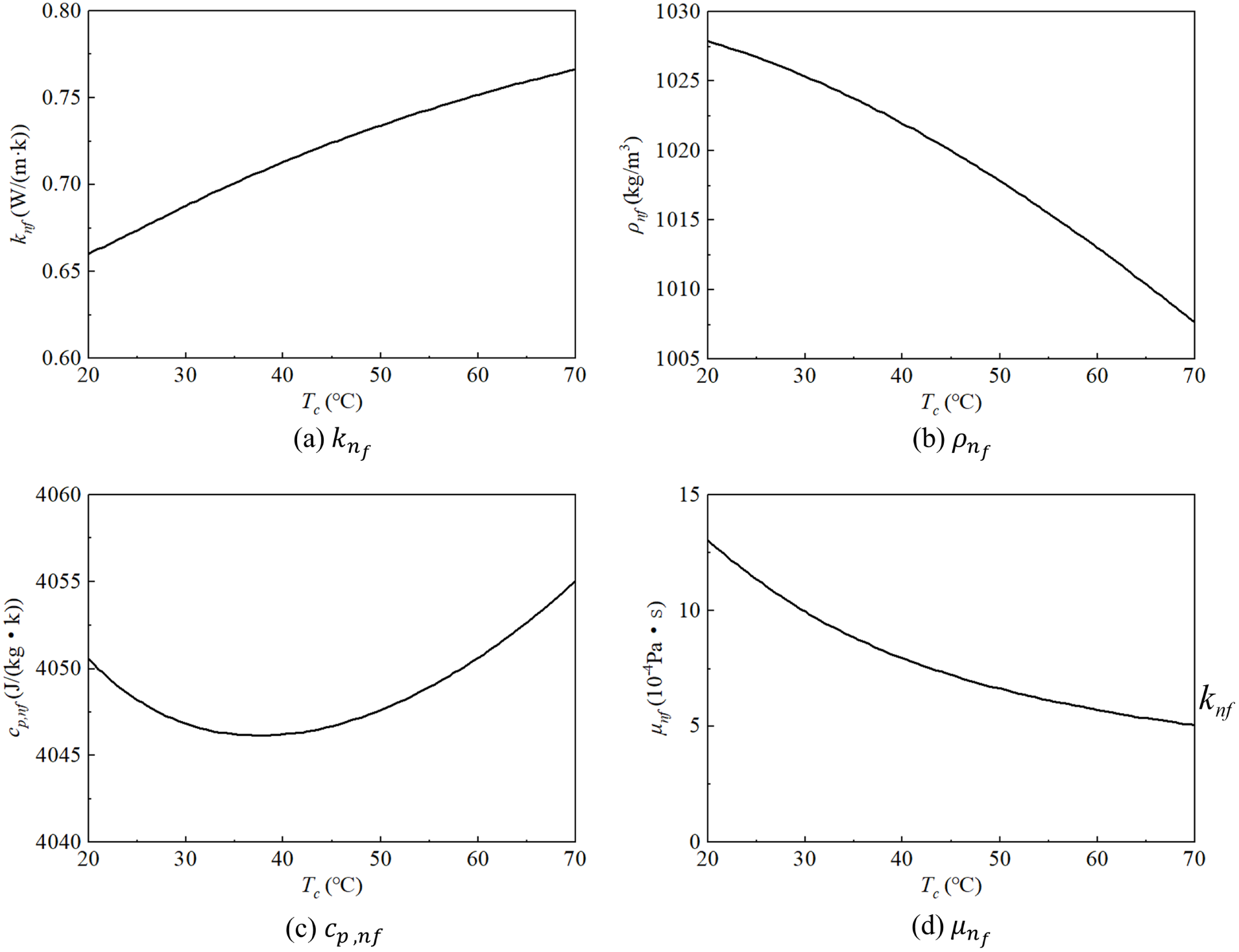
Figure 2: Temperature-sensitive thermophysical behaviors of the nanofluid with ϕp = 1% and dp = 13 nm.

2.3 Three-Layer Thermofluid Model

In this work, a steady thermofluid problem is investigated, and the flow is taken as incompressible and laminar inside the NCMHS. Furthermore, the flow is taken to be fully developed during the formulation of the three-layer model. The procedure from Zhao et al. [41] is used to derive the three-layer thermofluid model for the NCMHS.

2.3.1 Fluid Flow Model

In the thermofluid layer, the full 3D flow governing equations are expressed as

{∇⋅u=0ρnf(u⋅∇)u=−∇p+μnf∇2u,(9)

where u represents the 3D velocity field, and p represents the 3D pressure field. The mathematical simplification methods presented below refer to the work of Zhao et al. [41].

In the thermofluid channel, the velocity component in the z-direction is zero, and both the velocity components and pressure remain constant along the z-axis, i.e.,

uz=0,∂uz∂z=0,∂p∂z=0.(10)

The flow velocity at any point within the thermofluid channel can be determined by interpolating the velocity vectors at the intersection points where a line through the point along the z-direction crosses three distinct planes. A second-order Lagrangian interpolation polynomial is then applied to further interpolate these values, yielding the velocity field on any x-y plane. Given that Layer 1 and Layer 3 satisfy the no-slip boundary condition, the velocity field for an arbitrary x-y plane can be expressed as

u(z)=(z−z1)(z−z3)(z2−z1)(z2−z3)u(z2).(11)

With reference to Eqs. (10) and (11), Eq. (9) is simplified. By further setting z = z2, the flow governing equations defined on the thermofluid layer are derived as follows.

The continuity equation is defined as

∂ux∂x+∂uy∂y+0=0.(12)

The momentum equation in the x-direction is given as

ρnfux(z2)∂ux(z2)∂x+ρnfuy(z2)∂ux(z2)∂y=−∂p(z2)∂x+μnf(∂2ux(z2)∂x2+∂2ux(z2)∂y2+2ux(z2)(z2−z1)(z2−z3)).(13)

The momentum equation in the y-direction is given as

ρnfux(z2)∂uy(z2)∂x+ρnfuy(z2)∂uy(z2)∂y=−∂p(z2)∂y+μnf(∂2uy(z2)∂x2+∂2uy(z2)∂y2+2uy(z2)(z2−z1)(z2−z3)).(14)

The momentum equation in the z-direction vanishes.

It can be seen that the flow governing equations are decoupled in the z-direction, which can also be written as

{∇⋅u2d=0ρnf(u2d⋅∇)u2d=−∇p2d+μnf∇2u2d+Kνu2d,(15)

where u2d and p2d represent the 2D velocity field and 2D pressure field at the central cross-section of the thermofluid channel, respectively, and ∇ is the 2D gradient operator. Compared to the 2D N-S equations, Eq. (15) includes an additional body force term with a coefficient of Kν=2μnf(z2−z1)(z2−z3).

The Neumann boundary condition for the flow problem is expressed as

nT(−p2dI+μ(∇u2d+(∇u2d)T))n=−p0,(16)

where n represents the outward normal vector on the boundary, and I is the unit tensor.

The schematic diagram of the design domain and boundary conditions of the NCMHS is shown in Fig. 3, which is highly consistent with the relevant settings reported in [30]. Ω represents the fluid domain, Γin and Γout are the inlet and outlet boundaries, respectively, Γw is the boundary of the design domain wall, and ΓS is the boundary of the solid-fluid wall. Pressure boundary conditions are defined at Γin and Γout, and the velocity boundary condition at ΓS and Γw is defined as no-slip in the form of

{u2d=0,on ΓS∪ΓW,p0=Δp,on Γin,p0=0,on Γout,(17)

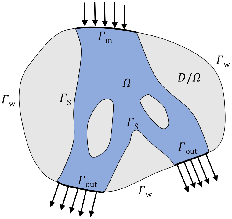
Figure 3: Schematic diagram of the design domain and boundary conditions of the NCMHS.

2.3.2 Heat Transfer Model

The schematic representation in Fig. 4 demonstrates the reciprocal thermal coupling phenomena between successive layers, where gray regions stand for solid domains while blue areas denote fluid zones. The established heat transfer framework covers not only the heat transport processes inside each individual layer but also the interfacial thermal linkage between nearby layers. Qijs and Qijf represent the coupled heat fluxes between the solid or fluid regions of layer i and layer j.

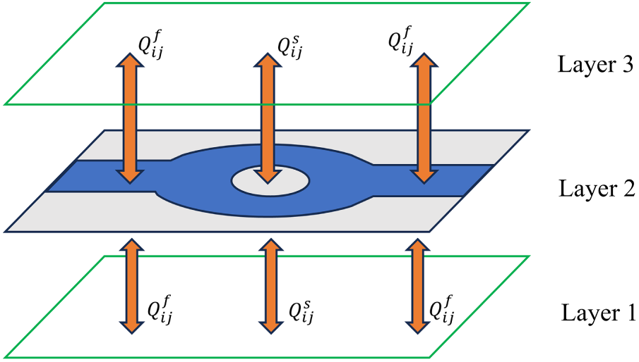
Figure 4: Schematic diagram of the coupled thermofluid influences between adjacent layers.

Afterwards, with the help of the derivation technique introduced in the work of Zhao et al. [41], the governing equations describing heat transfer in the first three layers can be formulated in the form shown below.

Layer 1:

{d1∇⋅(ks∇T1)+d1Qs+Q12s=0d1∇⋅(ks∇T1)+d1Qs+Q12f=0(18)

Layer 2:

{d2∇⋅(ks∇T2)+Kc(Q21s+Q23s)=0d2∇⋅(knf∇T2)+Kc(Q21f+Q23f)=d2ρnfcp,nfu2d⋅∇T2(19)

Layer 3:

{d3∇⋅(ks∇T3)+Q32s=0d3∇⋅(ks∇T3)+Q32f=0(20)

where di(i=1,2,3) represents the thickness of layer i, ks and knf represent the thermal conductivity of the solid and nanofluid, respectively, and Ti(i=1,2,3) represents the 2D temperature field of layer i. The thermal conductivity of the solid is ks=50W/(m⋅K). Qs represents the heat source applied to Layer 1. A temperature-sensitive heat source proposed by Matsumori et al. [28] is used, assuming an ideal heat source at temperature TQ, with heat flow input from the bottom plate’s bottom boundary. The heat generation rate is proportional to the temperature difference between the heat source and the bottom plate, expressed as:

Qs=β(TQ−T1),(21)

where β is the heat generation coefficient controlling the heat generation rate, and the heat source temperature is set to TQ=340 K. Kc is the correction factor for the coupled heat fluxes between Layer 2 and adjacent layers, and its value depends on the boundary conditions set for the problem. The Kc will be specifically determined in Section 2.3.3.

According to the assumption made by Zhao et al. [41], the temperature at any point within the thermofluid channel can be determined by interpolating the temperature values at the intersections of the line that passes through the point along the z-direction with three distinct planes. The resulting second-order Lagrange interpolation expression for the temperature field as a function of z is given as

T(x0,y0,z)=∑i=13T(x0,y0,zi)∏1≤i≤3z−zjzi−zj.(22)

By combining Fourier’s law and Eq. (22), the coupled heat flux Qij is derived as follows.

Layer 1:

{Q12s=−ks∂T∂z|z=z1=−ks(2z1−z2−z3(z1−z2)(z1−z3)(T1−T2)+z1−z2(z3−z1)(z3−z2)(T3−T2))Q12f=−knf∂T∂z|z=z1=−knf(2z1−z2−z3(z1−z2)(z1−z3)(T1−T2)+z1−z2(z3−z1)(z3−z2)(T3−T2))(23)

Layer 3:

{Q32s=−ks(−∂T∂z|z=z3)=ks(z3−z2(z1−z2)(z1−z3)(T1−T2)+2z3−z1−z2(z3−z1)(z3−z2)(T3−T2))Q32f=−knf(−∂T∂z|z=z3)=knf(z3−z2(z1−z2)(z1−z3)(T1−T2)+2z3−z1−z2(z3−z1)(z3−z2)(T3−T2))(24)

Layer 2:

{Q21=−Q12Q23=−Q32.(25)

The inlet temperature of the Al2O3-H2O nanofluid is set to Tin=293.15K, with adiabatic boundary conditions imposed on the wall, expressed as

{T=Tin, on Γin−n⋅∇T=0, on Γout∪ΓW.(26)

2.3.3 Determination of the Correction Factor Kc

This section discusses the determination of Kc. Fig. 5 shows the dimensions and domain setup of Layer 2 of the NCMHS, with the white and gray regions assigned to the fluid and solid subdomains correspondingly. The characteristic length L=1 mm. Leveraging the bilateral symmetry of the entire domain relative to the centerline, only the upper half is utilized as the effective computational domain, and symmetry boundary conditions are prescribed along the central symmetry axis.

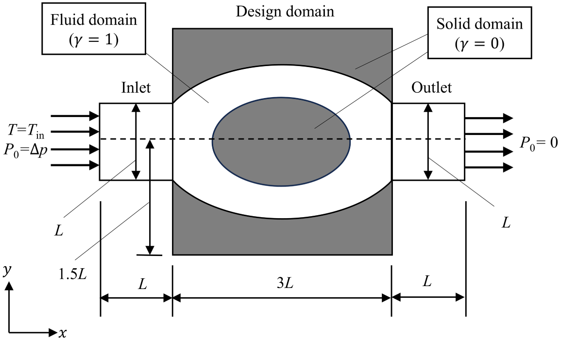
Figure 5: Dimensions and domain setup of Layer 2 of NCMHS.

The plane cooling channel with three parallel fins (as shown in Fig. 6) is selected as the 2D model for Layer 2. The finite element computations are carried out using both the three-layer and fully 3D thermofluid coupling models. ϕp = 1%, dp = 36 nm, β = 108 W/(m3∙K) and Δp = 100 Pa are used. The average temperature in the design domain of Layer 1 is adopted as the evaluation criterion, which can be expressed as

Tave=∫DT1dx/∫D1 dx,(27)

where D is the design domain of Layer 1.

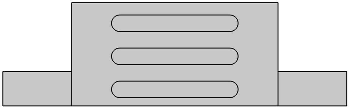
Figure 6: Plane cooling channels with three parallel fins.

Table 1 lists the values of parameter Tave under different Kc conditions. Analysis of the tabulated data indicates that when Kc = 1.3, the Tave value calculated by the three-layer thermofluid model is close to the result obtained from the full three-dimensional thermofluid model. Fig. 7 presents the temperature field of the first layer predicted by the two models at Kc = 1.3. Evidently, the temperature distributions derived from the two numerical models show satisfactory consistency.

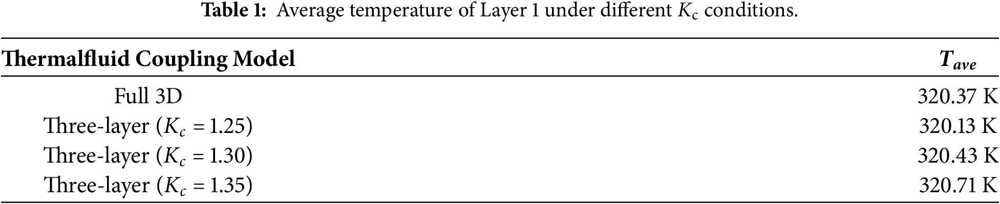
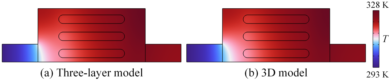
Figure 7: Temperature fields in Layer 1 obtained using (a) the three-layer thermofluid model and (b) the fully 3D thermofluid model computed for the design shown in Fig. 6.

Furthermore, to ensure predictive fidelity under diverse pressure-drop boundary conditions, Kc values are calibrated for the specific operating conditions examined in this study using the procedure described above (Table 2).

3  Topological Optimisation

This work adopts the density-based approach to optimize the flow channel design of the NCMHS, with the aim of boosting its overall heat transfer capability. A design variable denoted as γ is defined to describe the virtual material density distributed in the design domain of the thermofluid layer. This variable γ is a continuous quantity that spans the interval from 0 to 1, with 0 representing the solid phase and 1 corresponding to the fluid phase.

3.1 Modified Three-Layer Thermofluid Model

To facilitate subsequent topological optimisation, the preceding governing equations are reformulated to incorporate design variables.

First, based on the research by Borrvall and Petersson [14], a body force term is used to Eq. (15) and one obtains

{∇⋅u2d=0ρnf(u2d⋅∇)u2d=−∇p2d+μnf∇2u2d+Kνu2d−α(γ)u2d,(28)

where α(γ) stands for the inverse permeability of the porous medium, which is given as

α(γ)=αmaxq(1−γ)q+γ,(29)

where q=0.01 denotes a tuning parameter. αmax has the form of

αmax=(1+1Re)μinDa⋅L2,(30)

where the Darcy number is Da=10−4, and Re represents the Reynolds number, expressed as

Re=ρinUinLμin(31)

We have

Uin=∫Γin|u2d|dΓ/L,ρin=∫ΓinρnfdΓ/L,μin=∫ΓinμnfdΓ/L(32)

The interpolation can be used for the heat transfer model as

Layer 1:

d1∇⋅(ks∇T1)+d1Qs+Q12(γ)=0,(33)

Layer 2:

d2∇⋅(k(γ)∇T2)+Kc(Q21(γ)+Q23(γ))=d2γρnfcp,nfu2d⋅∇T2,(34)

Layer 3:

d3∇⋅(ks∇T3)+Q32(γ)=0,(35)

where Qij(γ) and k(γ) represent the coupled heat fluxes between layer i and layer j, and the thermal conductivity of Layer 2, respectively, which can be expressed as [52]

Qij(γ)=γ(Qijf(1+pc)−Qijs)+Qijs1+pcγ,(36)

k(γ)=γ(knf(1+pc)−ks)+ks1+pcγ,(37)

where pc=5.

3.2 Filtering and Projection

To restrict the complexity of the design, the Helmholtz equation [53] is used to filter out fine-scale design features. It can be expressed as follows:

{−r2∇2γf+γf=γ,in D∇γf⋅n=0,on ∂D,(38)

where r is specified as the mesh size and γf represents the design variable after filtering.

To prevent the emergence of blurred boundaries and non-manufacturable elements, the following function is used to project the design variables [54] as

γp=tanh⁡(βp(γf−γβ))+tanh⁡(βpγβ)tanh⁡(βp(1−γβ))+tanh⁡(βpγβ),(39)

where γp denotes the design variable after projection. γβ=0.5 determines the threshold of projection, so that design variables less than or greater than 0.5 are projected to 0 or 1, respectively. βp=8 is used.

3.3 Optimization Problem

This research takes the weighted average value of both the mean temperature and the peak temperature in the design domain of Layer 1 as the objective function, and its specific expression is as follows

J(f,γ)=w∫DT1dx∫D1 dx+(1−w)(∫DT1Ndx∫D1 dx)1/N(40)

where the peak temperature is approximated by the p-norm of the temperature field over the design domain of Layer 1 with N = 10. w is the weight coefficient. f denotes the state vector, taken as f = (u2d,x, u2d,y, p2d, T1, T2, T3). The weak form of the governing equations for the three-layer thermofluid model can be expressed as

E1(f,γp)=−∫Dp2d′∇⋅u2ddx=0(41)

E2(f,γp)=∫Dρnf(u2d⋅∇)u2d⋅u2d′dx−∫Dp2d∇⋅u2d′dx+∫Dμnf(∇u2d):(∇u2d′)dx+∫Dα(γp)u2d⋅u2d′−Kνu2d⋅u2d′dx+∫∂D(p2dI−μnf∇u2d)n⋅u2d′ds=0(42)

E3(f,γp)=−∫Dd1ks∇T1⋅∇T1′dx+∫Dd1QsT1′dx+∫DQ12(γp)T1′+∫∂Dd1ks∇T1⋅nT1′ds=0(43)

E4(f,γp)=∫Dd2γpρnfcp,nf(u2d⋅∇)T2T2′dx+∫Dd2k(γp)∇T2⋅∇T2′dx−∫DKc(Q21(γp)+Q23(γp))T2′dx−∫∂Dd2k(γp)∇T2⋅nT2′ds=0(44)

E5(f,γp)=−∫Dd3ks∇T3⋅∇T3′dx+∫DQ32(γp)T3′+∫∂Dd3ks∇T3⋅nT3′ds=0(45)

E6(γf,γ)=∫Dr2∇γf⋅∇γf′dx+∫Dγfγf′dx−∫Dγγf′dx=0(46)

E7(γf)=tanh⁡(βp(γf−γβ))+tanh⁡(βpγβ)tanh⁡(βp(1−γβ))+tanh⁡(βpγβ)=γp(47)

where γf′, u2d′, p2d′, T1′, T2′ and T3′ are the test functions corresponding to γf, u2d, p2d T1, T2 and T3, respectively. The topological optimisation problem can be described as

Minimize:J(f(γ),γ)Subject to:{E1(f(γp),γp)=0E2(f(γp),γp)=0E3(f(γp),γp)=0E4(f(γp),γp)=0E5(f(γp),γp)=0E6(γf,γ)=0E7(γf)=γp0≤γ≤1(48)

3.4 Sensitivity Analysis

In the present work, the adjoint sensitivity analysis approach is utilized to acquire the gradient information required for updating the design variable γ. To begin with, we compute the Eulerian derivative of the objective function J(f, γ) with respect to the design variable γp as

dJ(f,γ)dγp=∂J(f,γ)∂γp+(∂J(f,γ)∂f)T∂f∂γp(49)

The residual of the governing equations can be obtained from the weak forms as

E(f,γp)=E1(f,γp)+E2(f,γp)+E3(f,γp)+E4(f,γp)+E5(f,γp)=0(50)

The Euler derivative is taken on both sides of Eq. (50) with respect to γp as

dE(f,γp)dγp=∂E(f,γp)∂γp+(∂E(f,γp)∂f)∂f∂γp=0(51)

From (51), it can be deduced that

∂f∂γp=−(∂E(f,γp)∂f)−1∂E(f,γp)∂γp(52)

Substituting (52) into (49), we get

dJ(f,γ)dγp=∂J(f,γ)∂γp−(∂J(f,γ)∂f)T(∂E(f,γp)∂f)−1∂E(f,γp)∂γp(53)

Introducing the adjoint variable ω, we can obtain the adjoint equation as

(∂E(f,γp)∂f)ω=(∂J(f,γ)∂f)(54)

Then (53) can be rewritten as

dJ(f,γ)dγp=∂J(f,γ)∂γp−ωT∂E(f,γp)∂γp(55)

The gradient information can be derived using the chain rule as

dJ(f,γ)dγ=(∂J(f,γ)∂γp−ωT∂E(f,γp)∂γp)⋅dγpdγf⋅dγfdγ(56)

3.5 Numerical Implementation

The thermophysical properties of nanofluids are dependent on temperature, which makes the thermofluid model we investigate a typical bidirectionally coupled system. Specifically, the velocity field can influence the temperature distribution through the convective term in the Layer 2 heat transfer governing equation from the corresponding formula. Meanwhile, temperature fluctuations will change the nanofluid’s thermophysical properties, and then regulate the dynamic behavior of the fluid flow. This kind of reciprocal interaction results in a strong coupling influence between the flow and heat transfer processes. For the purpose of obtaining more accurate numerical solutions, we employ a fully coupled finite element method to handle these governing equations.

Topological optimisation is performed using a numerical iterative approach. The flowchart in Fig. 8 illustrates this numerical iterative process, which is similar to that in reference [30]. First, the design variables γ and other parameters are initialized. Subsequently, the governing physical equations, i.e., Eqs. (28) and (33)–(35) are solved. The objective function is then computed. Convergence is checked to decide whether to proceed to the next iteration. In this study, the convergence criterion is specified as a variation in the objective function smaller than 0.001. If convergence is not achieved, the sensitivity analysis is performed, and the design variables are renewed using the globally convergent method of moving asymptotes (GCMMA) [55]. The internal tolerance factor and constraint penalty factor of the GCMMA algorithm are set to 0.1 and 1000, respectively. Finally, regularization is carried out using Eqs. (38) and (39). This iterative process continues until either the convergence criterion is satisfied or the maximum number of iterations is reached, thereby completing the optimization.

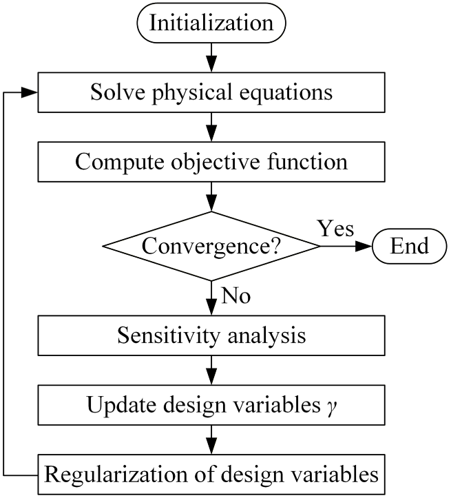
Figure 8: Flowchart of the proposed optimization procedure.

4  Numerical Examples

Topological optimisation for NCMHS is implemented in this section, relying on the established three-layer thermofluid model, to clarify the optimized structural patterns under diverse operating circumstances.

4.1 Influences of the Weight Coefficient on Optimized Designs

We first study a typical optimization case where w = 0.5, ∆p = 200 Pa, and β = 108 W/(m3∙K). ϕp = 1% and dp = 36 nm are set. The design variable γ is initially assigned a value of 0.5. The computational domain is discretized using 14,716 rectangular mesh elements. The influence of the number of grid elements on the optimized design is provided in Supplementary File S1 of the Supplementary Material. From Fig. 9, we can see that the objective function gradually decreases with the increasing number of iterations and stabilizes once the convergence criterion is satisfied. Fig. 10 shows the distribution of the design variable γ at selected iterations. Fig. 11 presents the distribution of velocity and temperature in Layer 2 at various iteration stages. The optimization process evolves as follows. Within the first 8 iterations, the gray area of the initial design decreases alongside an increase in nanofluid velocity. Between iterations 8 and 20, island-like solid regions form in the design domain, leading to more flow channels and an expanded fluid-solid heat transfer area. From iteration 20 to 30, intermediate densities are binarized to 0 and 1, and boundary jagged features are removed. Clear flow channels are thus formed in the following iterations.

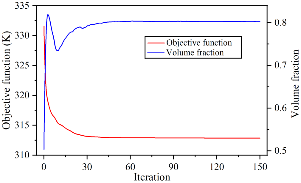
Figure 9: Convergence histories for a typical optimization case.

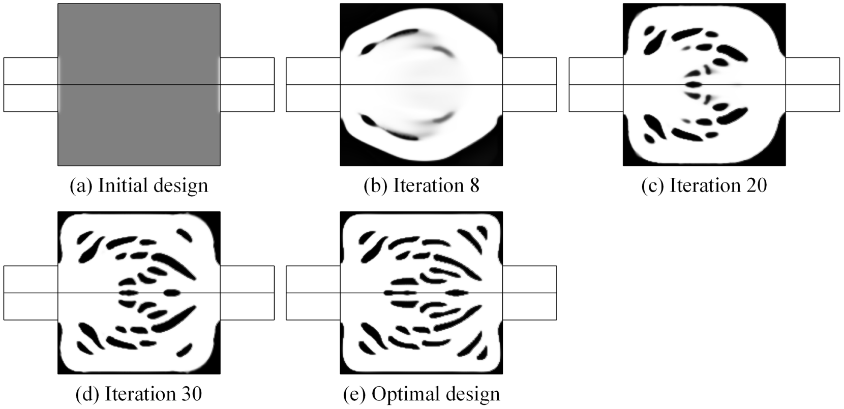
Figure 10: Distributions of the design variable γ at different iterations.

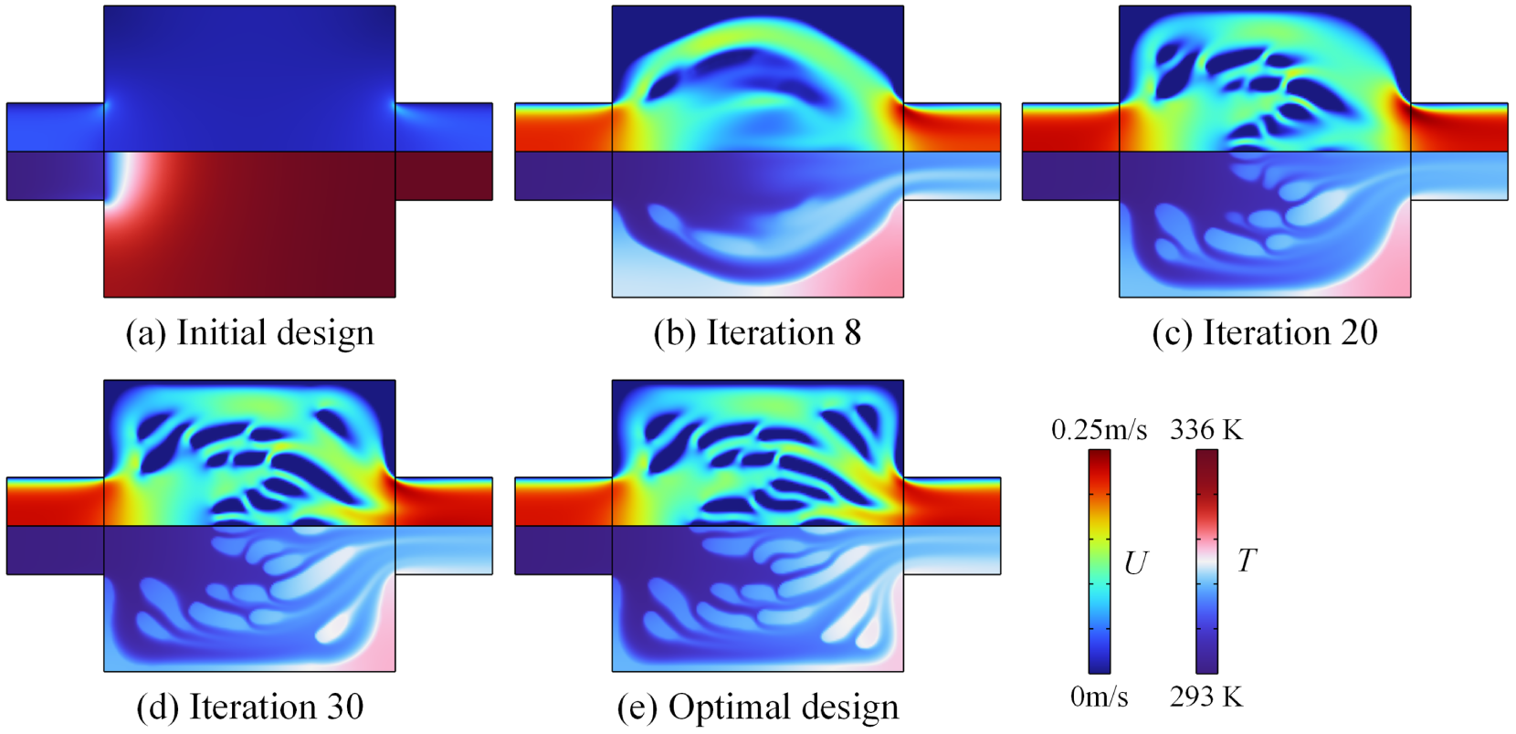
Figure 11: Velocity and temperature distributions for the designs shown in Fig. 10.

To investigate the influences of the weight coefficient on the optimized designs, additional topological optimisation cases with w = 0, 0.2, 0.8, and 1 are examined under the optimization settings described above. Figs. 12–14 present the optimized designs, the temperature distributions in Layer 1, and the velocity and temperature distributions in Layer 2 for different weight coefficient cases, respectively. Table 3 lists the values of ξ, J, Tave and Tm for the optimized designs shown in Fig. 12, where Tm denotes the maximum temperature in the design domain of Layer 1. ξ denotes the fluid volume fraction within the design domain of Layer 2.

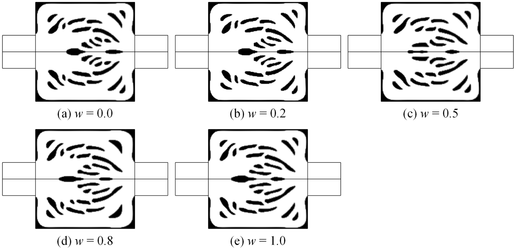
Figure 12: Optimized designs with different values of weight coefficient.

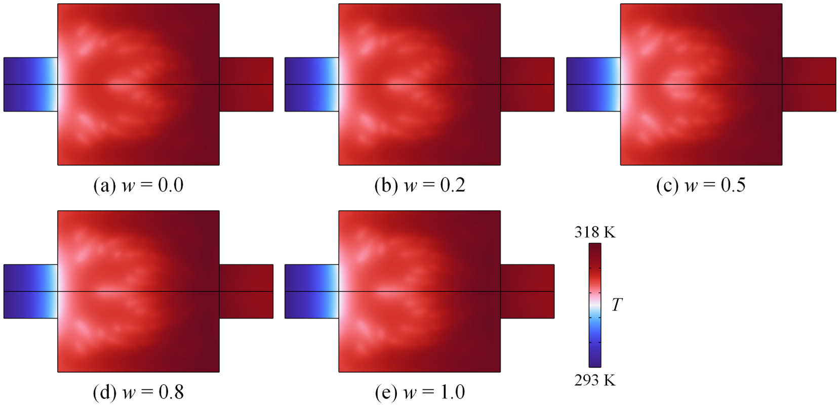
Figure 13: Temperature distributions in Layer 1 for optimized designs in Fig. 12.

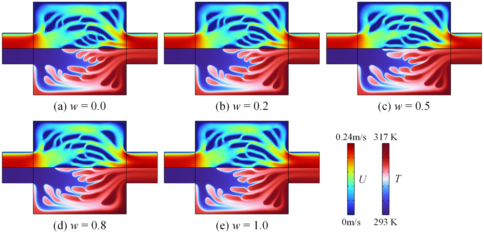
Figure 14: Velocity and temperature distributions in Layer 2 for optimized designs in Fig. 12.

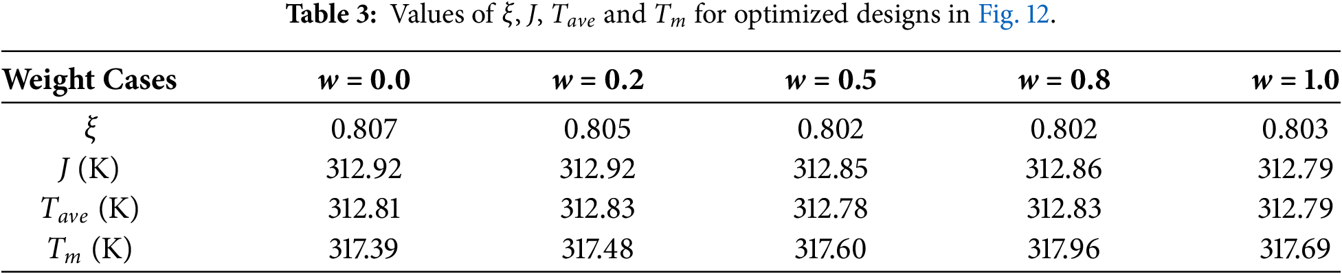
As can be seen from Fig. 12, the optimized designs obtained with different weight coefficients exhibit only minor differences, and their structural features are quite similar. Likewise, Figs. 13 and 14 show that the temperature and velocity fields corresponding to these designs are also very similar. Furthermore, the data in Table 3 indicate that the objective function values, as well as the average and maximum temperatures in the design domain of Layer 1, differ only negligibly among the optimized designs for different weight coefficients.

This may be attributed to the fact that, for the optimized designs under different weight coefficients, the temperature distribution in the design domain of Layer 1 is relatively uniform (as confirmed by the temperature distributions in Fig. 13). Consequently, the two terms constituting the objective function, i.e., Tave and the p-norm of the temperature field, take closely comparable values, which may render the optimized design results largely insensitive to variations in the weight coefficient.

4.2 Influences of Temperature-Sensitive Fluid Properties on Optimized Designs

In this section, Δp = 200 Pa, β = 108 W/(m3∙K), w = 0.5, ϕp = 1% and dp = 36 nm are used. The optimized results of the nanofluid with temperature-sensitive properties are shown in Fig. 15a and Fig. 15e, respectively. To facilitate the comparison of results, coolants with constant fluid properties are introduced, and corresponding topological optimisation studies are conducted. Eqs. (1)–(4) are used to compute the thermophysical properties of the fluid under this constant temperature condition, where the original variable temperature is replaced by a fixed temperature T0. Here, several representative constant temperatures are selected for T0, such as T0 = Tin, T0 = Tfa and T0 = Tq, where Tfa denotes the average temperature within the design domain for the temperature field shown in Fig. 15e. The computed values of dynamic viscosity for these constant problems are listed in Table 4. The optimized results under the constant conditions are also shown in Fig. 15. Table 5 presents the optimized results calculated using temperature-sensitive fluid properties to facilitate comparison.

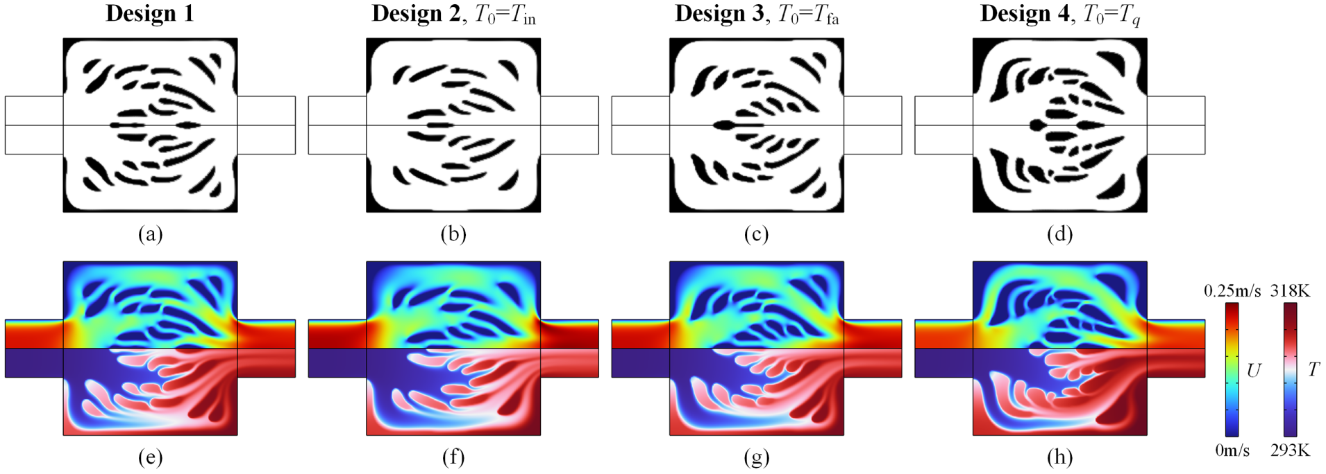
Figure 15: Optimized designs, and the corresponding flow velocity and temperature distributions for the temperature-sensitive problem and constant thermophysical problems. (a–d) correspond to the optimized designs for the temperature-sensitive problem (a) and constant thermophysical problems with the nanofluid properties at T0 = Tin (b), T0 = Tfa (c) and T0 = Tq (d). (e–h) show the velocity and temperature fields in Layer 2 correspond to the optimized designs in (a–d), respectively.

From Fig. 15, we can see that the optimized designs for the temperature-sensitive problem differ significantly from those for constant cases. This phenomenon may be attributed to the dynamic viscosity of nanofluids. As summarized in Table 4, the dynamic viscosity declines as T0 rises. It is well established that the pressure drop is proportional to the viscous dissipation of the fluid. Correspondingly, when the pressure drop remains consistent, the optimized design for high-viscosity working fluids generally employs a uncomplicated structural layout and sets aside a larger percentage of the flow field, which effectively alleviates the steep velocity gradient, which is distinctly reflected in the optimized design illustrated in Fig. 15. Design 2 has a simpler geometry and a larger fluid domain, which may contribute to a higher flow velocity (see Table 5). However, this design may reduce the heat transfer area. In contrast, Design 4 presents the opposite trend: its intricate design and more compact fluid domain expand the heat transfer surface, yet they bring about a relatively low flow velocity (see Table 5). As indicated by Fig. 15, the structural complexity of Design 1 is similar to that of Design 3, which lies between those of Design 2 and Design 4. Table 5 shows that the optimized result obtained by accounting for temperature-sensitive properties delivers the best overall heat transfer performance.

4.3 Influences of the Pressure Drop ∆P on Optimized Designs

In this section, ϕp = 1%, dp = 36 nm, β =108 W/(m3∙K) and w = 1 are used. The optimized results for different pressure drops are shown in Figs. 16 and 17. Table 6 provides a set of critical data for each corresponding optimized design. The variation trend of optimized designs in Fig. 16 indicates that the number of branch channels within the flow domain increases progressively with the rise in pressure drop. Under low pressure drop conditions, cooling performance may be primarily improved by raising flow velocity, which may be realized via optimized designs featuring fewer branch channels. With the gradual increase of pressure drop, the nanofluid obtains a more powerful flow driving force. Thus, it is capable of overcoming the flow resistance brought by the complex branch channels while keeping a high flow rate. In turn, more intricate branching flow channels are generated under higher pressure drops, which expands the heat transfer area and further optimizes the heat transfer performance of the NCMHS. As evidenced by Fig. 17 and Table 6, the flow rate are significantly enhanced at high pressure drops. Consequently, elevating the pressure drop remarkably improves the overall cooling performance of NCMHS, resulting in a continuous reduction of the objective function.

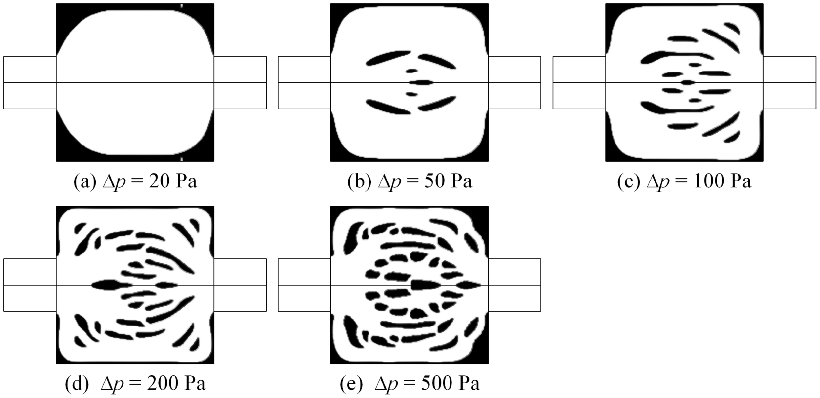
Figure 16: Optimized designs for optimization problems with different pressure drops.

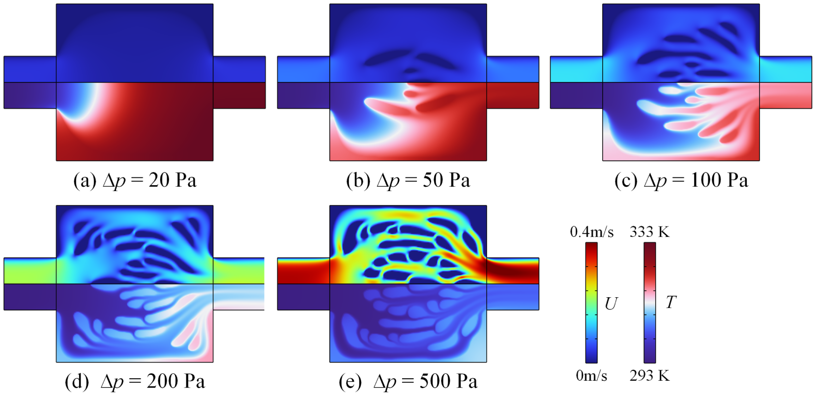
Figure 17: Velocity and temperature fields in Layer 2 for the optimized designs shown in Fig. 16.

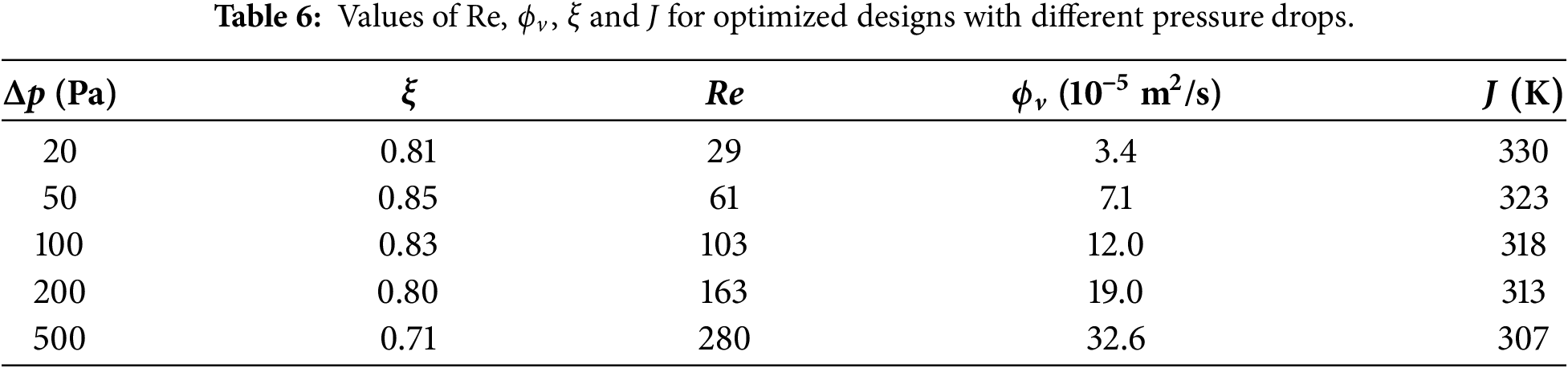
4.4 Validation of the Three-Layer Thermofluid Model

In this section, the proposed three-layer thermofluid model is validated using the optimized designs. The optimized geometries presented in Fig. 16 are numerically computed via both the three-layer simplified model and the full-scale 3D thermofluid model under their respective specified pressure drop conditions. The optimized design shown in Fig. 16 is extruded in the thickness direction and then assembled with the bottom and top plates to construct a fully integrated three-dimensional heat sink. Body-fitted grids are used for these two models. The material properties, heat source, and boundary conditions adopted in the numerical simulations are consistent with those described in Section 4.3. Based on this precondition, the numerical calculation procedures are re-conducted via the finite element method. The corresponding grid independence tests for both models are provided in Section S2 of the Supplementary Material.

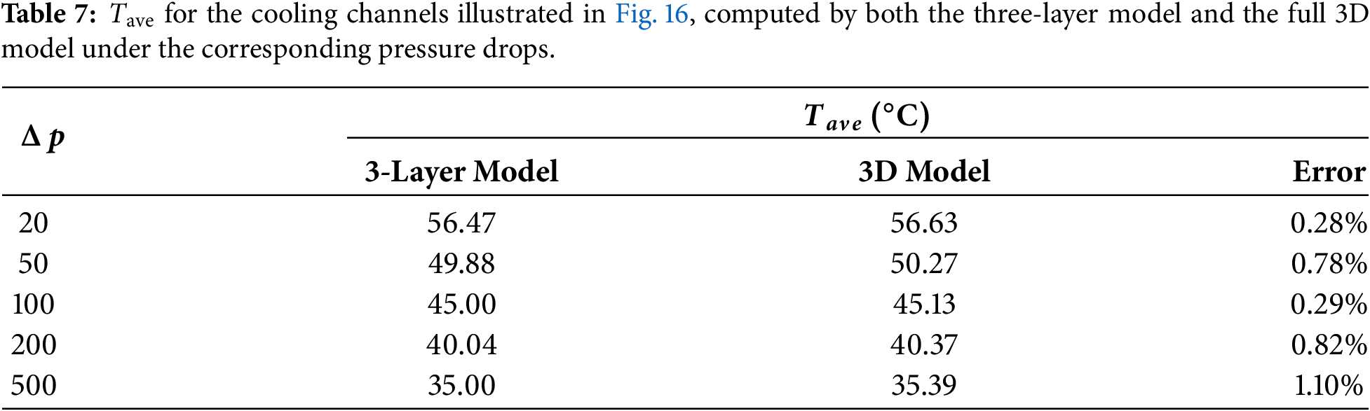
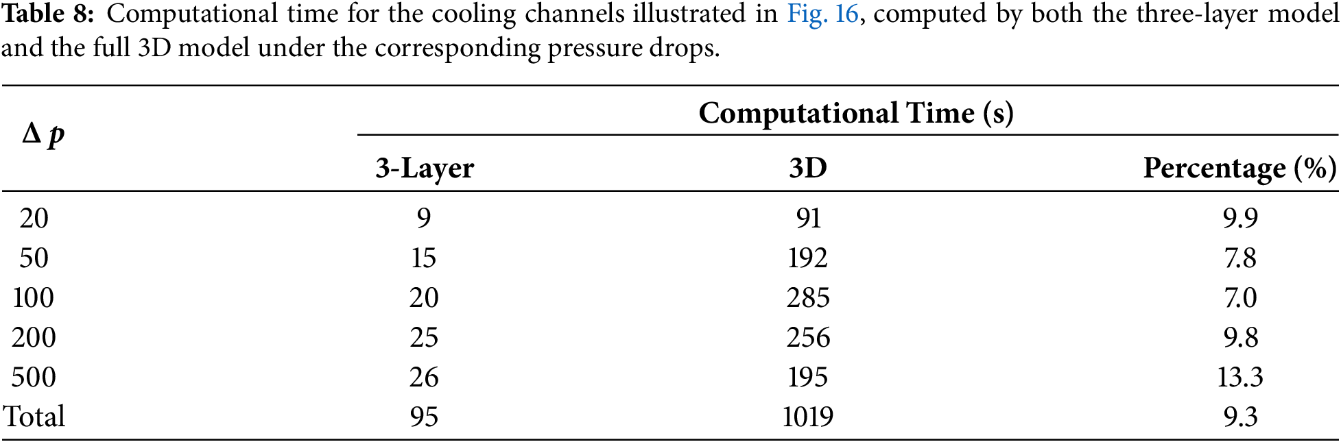
Figs. 18 and 19 show the temperature field in Layer 1, and the velocity and temperature fields in Layer 2, respectively, as computed by the two models when ∆p = 100 Pa. Table 7 shows Tave for the cooling channels illustrated in Fig. 16 computed by the two models. The outcomes obtained in this study show a strong and consistent match between the newly established three-layer model and the full three-dimensional numerical model. A detailed comparison of the time consumption required for calculation under different pressure drop scenarios is summarized in Table 8, where all simulations are run on an identical hardware configuration equipped with an Intel(R) Core(TM) i9-11900 2.50 GHz CPU and 128 GB RAM. As clearly illustrated in the table, the presented three-layer structure cuts down the mean calculation duration by over 90% relative to the fully 3D counterpart. This finding further verifies that the introduced simplification strategy can realize a dramatic drop in computational overhead while maintaining high prediction precision.

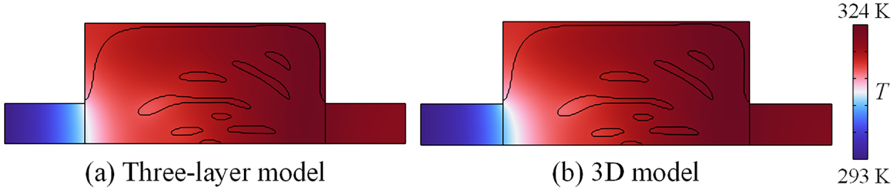
Figure 18: The temperature fields in Layer 1 for the cooling channel illustrated in Fig. 16c, computed by the three-layer thermofluid model (a) and the full 3D thermofluid model (b) when ∆p = 100 Pa.

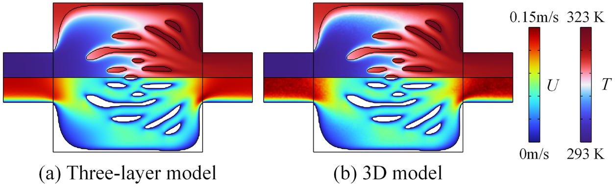
Figure 19: The velocity and temperature fields in Layer 2 for the cooling channel illustrated in Fig. 16c, computed by the three-layer thermofluid model (a) and the full 3D thermofluid model (b) when ∆p = 100 Pa.

4.5 Influences of the Heat Source on Optimized Designs

In this section, the influences of heat sources on the optimization results are investigated, including the magnitude of the heat generation coefficient, the distribution locations and geometries of heat sources. Δp = 200 Pa, w = 0.5, ϕp = 1% and dp = 36 nm are used.

4.5.1 Influences of β on Optimized Designs

As shown in Eq. (21), when TQ is fixed, β directly determines the magnitude of the heat generation amount. The optimized results for different β are shown in Figs. 20 and 21. The data in Table 9 include the Reynolds number Re, nanofluid volume fraction ξ within the design domain, average dynamic viscosity of the nanofluid μ¯nf within the design domain, objective function value J, and flow rate ϕv corresponding to the different results in Fig. 21. μ¯nf can be calculated as

μ¯nf=∫Dμnfdx/∫D1 dx.(57)

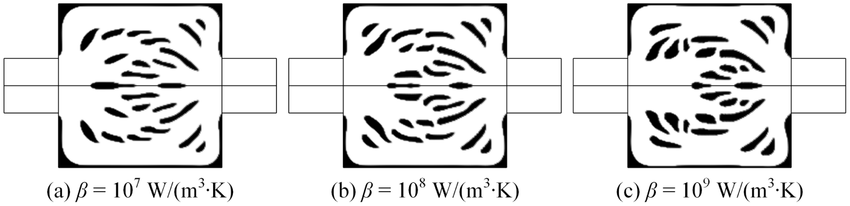
Figure 20: Optimized designs for different β.

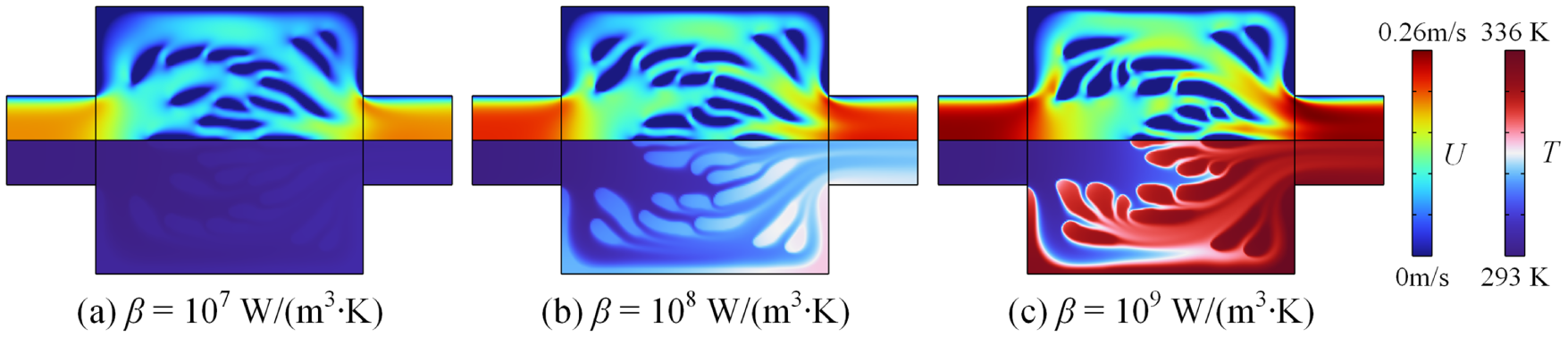
Figure 21: Velocity and temperature fields in Layer 2 for different β.

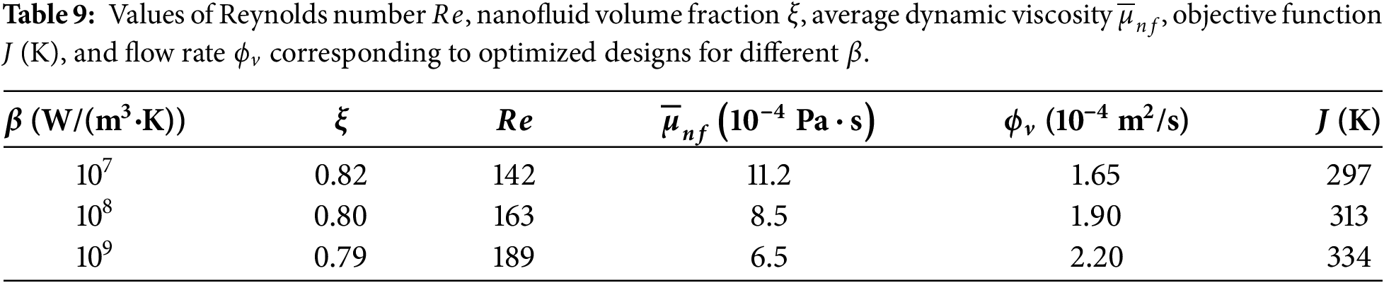
The optimized designs in Fig. 20 show that certain differences exist among the optimized designs obtained under different heat generation coefficients. These differences may be attributed to the temperature-sensitive characteristics of the dynamic viscosity of nanofluid. The data in Table 9 show that as β increases, the average dynamic viscosity of the nanofluid μ¯nf within the design domain gradually decreases. Specifically, when β is large, more heat may be introduced from the bottom plate into the thermofluid channel of the NCMHS, and the rise in temperature may lead to a reduction in the nanofluid dynamic viscosity. Given that the geometric complexity of the optimized designs exhibits negligible variation under different conditions (see Fig. 20), the decrease in dynamic viscosity may allow for a higher flow rate under identical pressure drop conditions, thereby enhancing heat transfer. This is supported by the flow rate data presented in Table 9. Therefore, under conditions with a higher heat generation coefficient, the thermal performance of the NCMHS may be primarily enhanced by increasing the flow velocity.

4.5.2 Influences of Heat Source Location on Optimized Designs

In certain special cases, excessive local power may lead to a nonuniform heat source distribution, thereby affecting the performance and safety of the system. In this section, the influences of different heat source locations on the optimized designs are discussed. The heat generation coefficient is set as β = 108 W/(m3∙K), and the heat source area is kept constant at a value of S=2 mm2 in all designs.

First, under the condition of a square heat source, the heat source is placed at the left, center, and right locations of the design domain for optimization, respectively. Fig. 22 shows the optimized designs with different heat source locations, while Fig. 23 shows the velocity and temperature distributions in Layer 2 corresponding to the optimized designs in Fig. 22. The objective function values corresponding to the optimized designs in Fig. 22a–c are 300, 299 and 298 K, respectively.

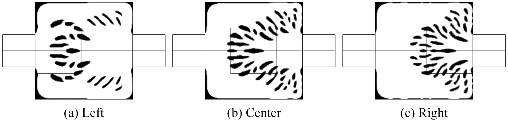
Figure 22: The optimized designs with the heat source located at the left (a), center (b), and right (c) of the design domain.

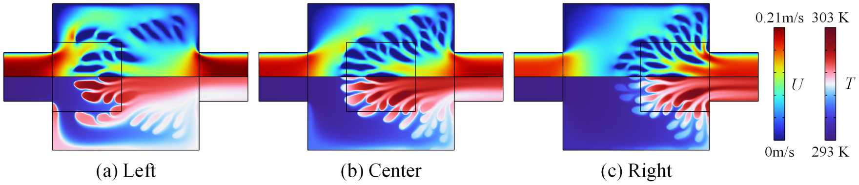
Figure 23: Velocity and temperature distributions in Layer 2 for the optimized designs shown in Fig. 22.

A clear pattern can be observed from the results in Fig. 22 that the solid fins are mainly located within and around the heat source regions. The heat dissipation process of the heat source can be divided into two sequential stages. In the first stage, heat entering through the bottom plate boundary is conducted through the solid substrate to the thermofluid channel layer. In the second stage, convective heat transfer within the thermofluid channel layer transports the heat away from the NCMHS. Given that the thermal conductivity of the solid substantially exceeds that of the fluid, a greater solid fraction within and around the heat source regions promotes rapid heat conduction from the bottom plate to the thermofluid channel layer. Meanwhile, the dispersed arrangement of multiple small solid fins increases the heat transfer area and further enhances the cooling performance of the NCMHS. The results in Fig. 23 show that as the heat source location approaches the outlet, the average temperature within the design domain decreases. The primary reason is likely that the fluid not passing through the heat source region exhibits a lower temperature. This observation is corroborated by the objective function values.

4.6 Influences of Nanofluid Features on Optimized Designs

In this section, the influences of the diameter and volume fraction of Al2O3 nanoparticles on the optimized designs are investigated. Furthermore, the differences in heat dissipation performance between the optimized designs of nanofluid and base fluid are compared and analyzed. w = 0.5, Δp = 200 Pa and β = 108 W/(m3∙K) are used.

4.6.1 Influences of the Nanoparticle Diameter on Optimized Designs

The nanoparticle volume fraction is fixed as ϕp = 1%. The optimized results for several typical nanoparticle diameters are presented in Figs. 24 and 25. Fig. 26 illustrates the influences of dp on the flow rate and the objective function. From Fig. 26, we can see that as the nanoparticle diameter increases, the heat transfer performance of the NCMHS generally increases. From the results in Fig. 24, it can be observed that the flow channel topology remains similar, indicating that the heat transfer area between the nanofluid and solid is not the main cause of the performance variation. However, from Fig. 26, we can see that the variation trend of the flow rate is generally opposite to that of the objective function. Consequently, the velocity variations arising from different nanoparticle diameters are likely the main reason affecting the cooling capability.

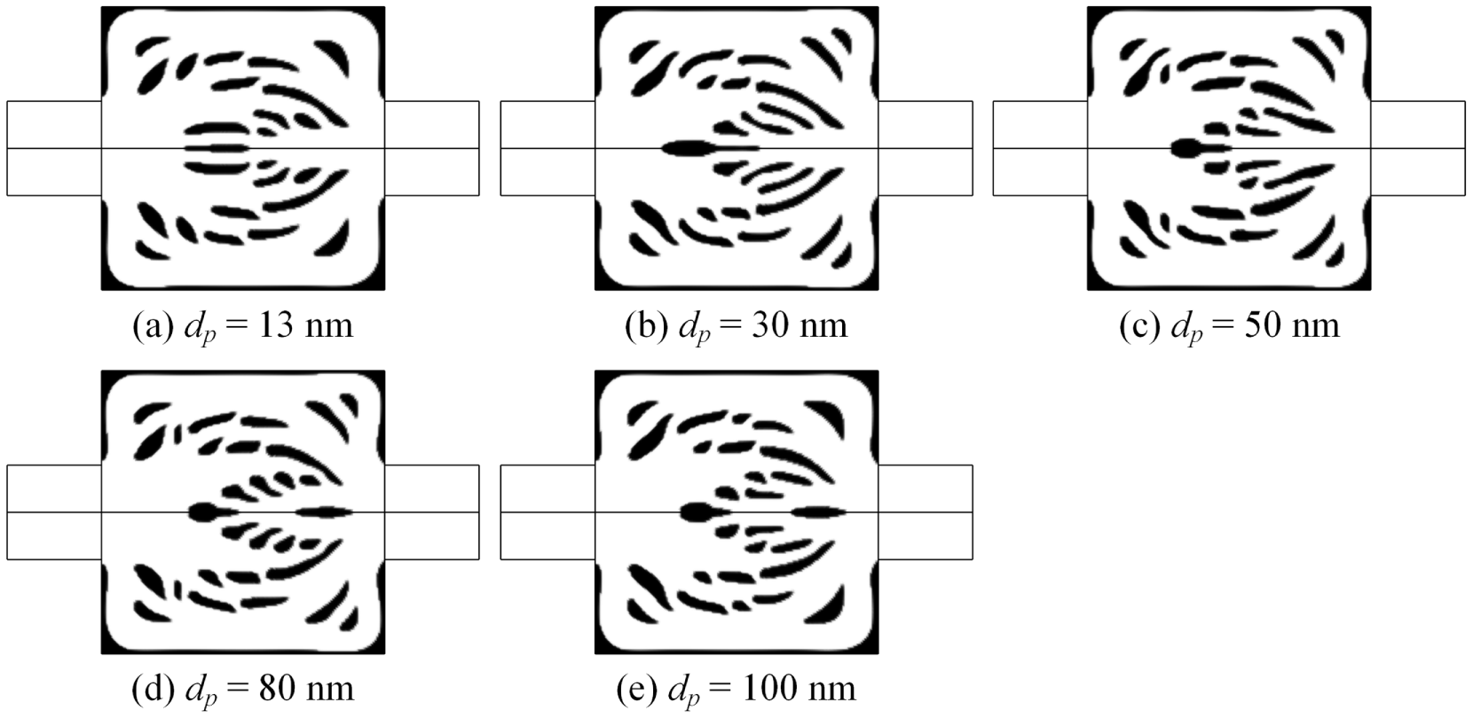
Figure 24: Optimized designs for typical nanoparticle diameters.

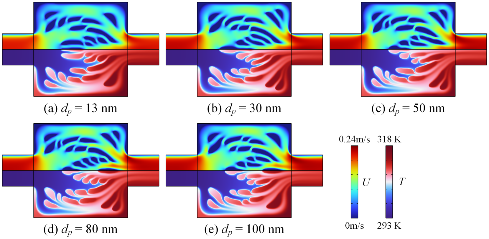
Figure 25: Velocity and temperature distributions of the results in Fig. 24.

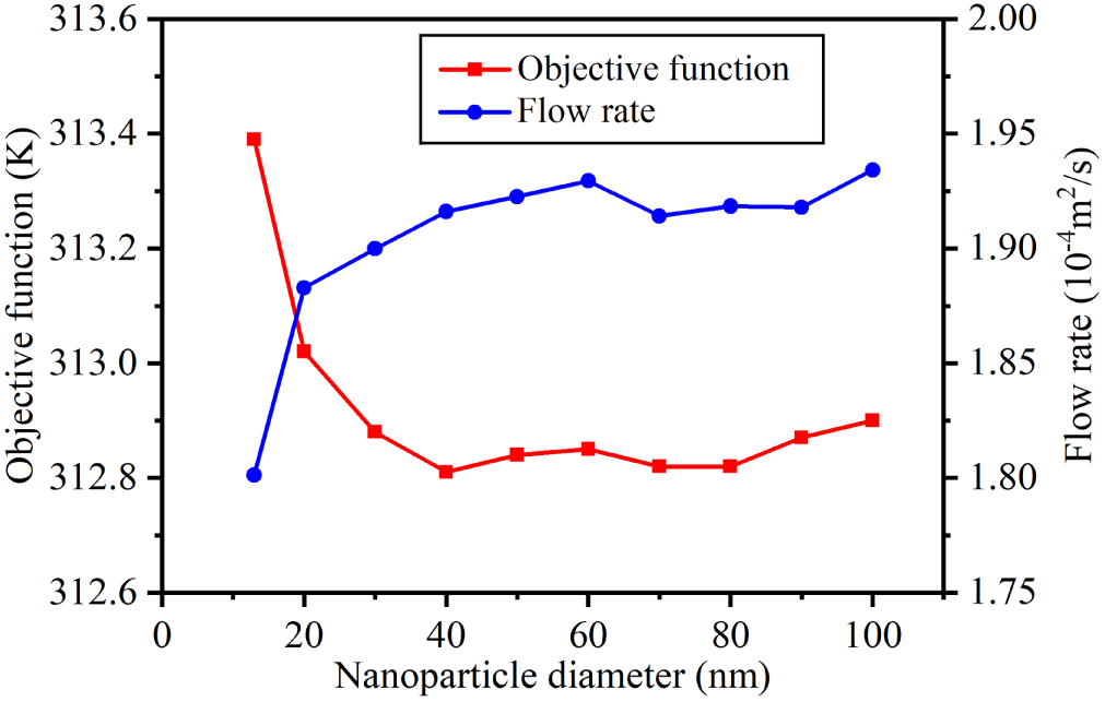
Figure 26: Influences of dp on the flow rate and the objective function of optimized designs.

4.6.2 Influences of the Nanoparticle Volume Fractions on Optimized Designs

dp=36nm is used. The optimized results for different ϕp are shown in Figs. 27 and 28. Fig. 29 illustrates the variation of the objective function and Re with ϕp. Fig. 29 presents the influence of ϕp on the characteristic dynamic viscosity μin and flow rate ϕv.

Figure 27: Optimized designs for different nanoparticle volume fractions.

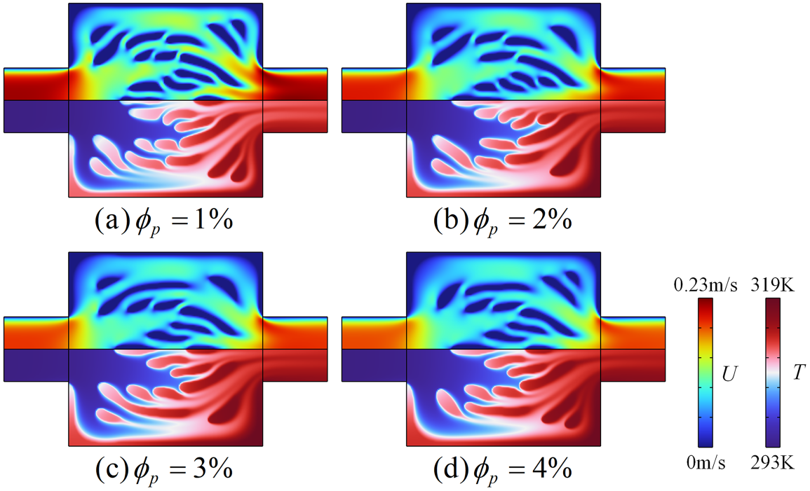
Figure 28: Velocity and temperature distributions for the optimized designs in Fig. 27.

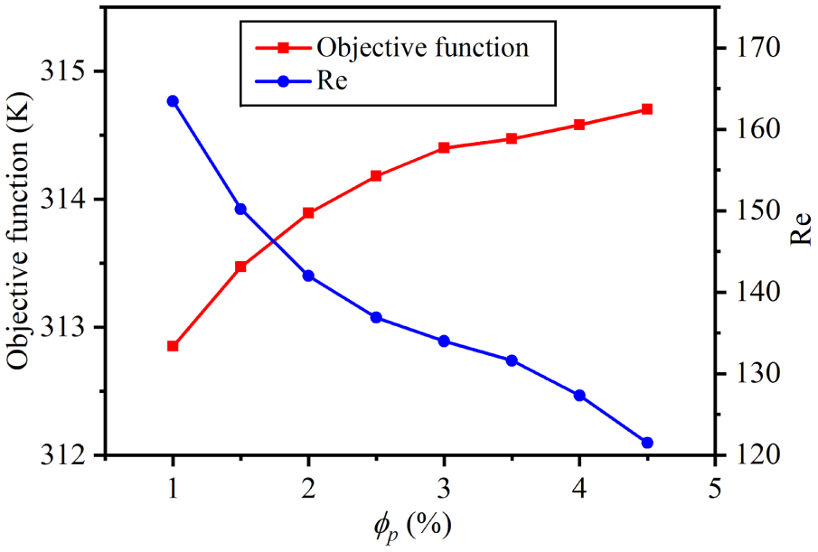
Figure 29: Influences of ϕp on the objective function and Re of optimized designs.

From the variation of the objective function in Fig. 29 and the velocity and temperature in Fig. 28 with respect to ϕp, it is evident that as ϕp increases, the heat transfer performance of the NCMHS decreases. The optimized designs in Fig. 27 show that the branched flow channels are reduced with the increase of ϕp, indicating that the convective heat transfer area between the nanofluid and solid decreases, which may be one cause of the decline in heat dissipation performance.

As shown in Fig. 30, increasing the nanoparticle volume fraction leads to a rise in μin and a corresponding decrease in flow rate. The reduction in flow rate may be another factor contributing to the decline in NCMHS performance.

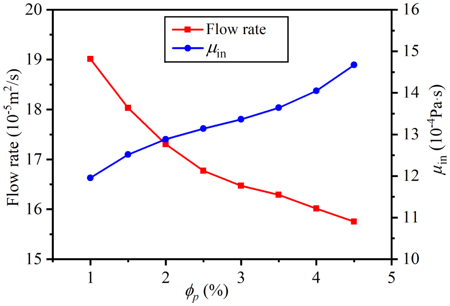
Figure 30: Influences of ϕp on ϕv and μin of optimized designs.

4.6.3 Topological Optimisation for the Base Fluid of the Nanofluid

To better investigate the influences of nanofluid properties on the optimized designs, the base fluid (H2O) is selected as the coolant for the topological optimisation design of NCMHS. The temperature-sensitive thermophysical properties of the nanofluid (ρnf, cp,nf, μnf, and knf) are replaced by those of the base fluid (ρbf, cp,bf, μbf, and kbf). Fig. 31 presents the optimized designs for the base fluid along with the corresponding velocity and temperature distributions. The data in Table 10 represent the μin, Re and ϕv of the base fluid. Compared with the results presented in Figs. 24 and 27, the optimized design shown in Fig. 31 exhibits more intricate flow channels. The optimized design corresponding to the base fluid not only features a more complex flow channel layout but also achieves a higher flow rate, which undoubtedly results in superior heat transfer performance. This performance enhancement may be largely attributed to the lower dynamic viscosity of the base fluid.

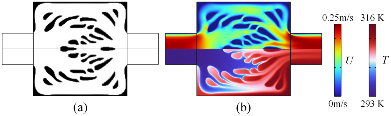
Figure 31: Optimized design and the velocity and temperature distributions in Layer 2 for the base fluid of the nanofluid, (a) optimized design, (b) velocity and temperature distributions.

5  Conclusions

In this study, a low-cost three-layer thermofluid model is employed to perform topological optimisation design of the cooling channels in the NCMHS. Numerical investigations are conducted to examine the influences of temperature-sensitive properties, pressure drop, heat source, and nanofluid characteristics on the NCMHS optimized designs. The main conclusions are as follows.

(1) A nanofluid with temperature-sensitive properties is employed as the coolant, and a three-layer thermofluid model for NCMHS is established in this work. Specifically, under the assumptions of the velocity profile and an adaptive temperature profile along the thickness direction, combined with the interlayer coupled heat flux deduced from Fourier’s law, the simplified thermofluid model is derived. The model fully considers the influences of out-of-plane flow boundaries and heat transfer characteristics. Under this modeling architecture, two-dimensional formulations are used to describe the conjugate heat transfer of the thermofluid layer, as well as heat conduction in the bottom and top plates. A density-based topological optimisation method is integrated into the model to obtain a three-layer topological optimisation method. The numerical results show that the optimized structure of NCMHS achieves a reasonable layout and improved heat dissipation capacity.

(2) The influences of temperature-sensitive fluid properties, pressure drop, heat source characteristics, and nanofluid properties on the optimized designs are numerically investigated. The results demonstrate that the optimized designs for nanofluids with temperature-sensitive properties differ significantly from those obtained under the constant-property assumption. As the pressure drop increases, the number of branched flow channels grows. Conversely, with increasing nanoparticle volume fraction, the complexity of branched flow channels in the optimized design decreases, and the heat transfer performance of the corresponding design decreases accordingly.

This study still has several limitations that merit further investigation in future work. First, a minimum length scale constraint could be incorporated into the topological optimisation process to effectively control structural feature sizes and filter out small, unintended design features, thereby yielding flow channel designs with improved manufacturability. Second, the current determination of the correction factor Kc relies on tedious empirical methods; therefore, more efficient and physically sound computational approaches need to be developed in future research.

Acknowledgement: None.

Funding Statement: This work is supported by the National Natural Science Foundation of China (Grant Nos. 52275272, 51905435 and 52475166), National Key Research and Development Program of China (Grant No. 2024YFE0204900) and China Postdoctoral Science Foundation (Grant Nos. 2020M683550 and 2022T150533).

Author Contributions: Bin Zhang contributed towards Supervision, Conceptualization, Methodology, Formulas, Software, Investigation, Writing—original draft and Writing—review & editing. Xuanyan Lu contributed towards Investigation, Software, Visualization, Validation and Writing—original draft. Zhigang Qin contributed towards Validation. Yibo Mo contributed towards Validation. Chenwei Wang contributed towards Validation and Writing—original draft. Sihui Hao contributed towards Writing—original draft. Yixiang Song contributed towards Validation. Jianyun Xu contributed towards Visualization. Zhifeng Zhang contributed towards Validation and Writing—review & editing. Xu Long contributed towards Supervision, Methodology, Validation and Writing—review & editing. All authors reviewed and approved the final version of the manuscript.

Availability of Data and Materials: The data that support the findings of this study are available from the Corresponding Authors, upon reasonable request.

Ethics Approval: Not applicable.

Conflicts of Interest: Given his role as Editorial Board Member of this journal, Xu Long had no involvement in the peer review of this article and had no access to information regarding its peer review. Full responsibility for the editorial process for this article was delegated to another journal editor. The authors declare no other conflicts of interest.

Supplementary Materials: The supplementary material is available online at https://www.techscience.com/doi/10.32604/cmes.2026.086481/s1.

References

1. Liu J, Liu D, Shang F, Yang K, Cao X, Zheng C. Study on heat transfer characteristics of pulsating heat pipe heat exchanger with asymmetric structure. Rev Int De Metodos Numer Para Calc Y Diseno En Ing. 2024;40(2):1–14. doi:10.23967/j.rimni.2024.05.005. [Google Scholar] [CrossRef]

2. van Erp R, Soleimanzadeh R, Nela L, Kampitsis G, Matioli E. Co-designing electronics with microfluidics for more sustainable cooling. Nature. 2020;585(7824):211–6. doi:10.1038/s41586-020-2666-1. [Google Scholar] [CrossRef]

3. Tuckerman DB, Pease RFW. High-performance heat sinking for VLSI. IEEE Electron Device Lett. 1981;2(5):126–9. doi:10.1109/edl.1981.25367. [Google Scholar] [CrossRef]

4. Wang XD, An B, Lin L, Lee DJ. Inverse geometric optimization for geometry of nanofluid-cooled microchannel heat sink. Appl Therm Eng. 2013;55(1–2):87–94. doi:10.1016/j.applthermaleng.2013.03.010. [Google Scholar] [CrossRef]

5. Wang XD, An B, Xu JL. Optimal geometric structure for nanofluid-cooled microchannel heat sink under various constraint conditions. Energy Convers Manag. 2013;65:528–38. doi:10.1016/j.enconman.2012.08.018. [Google Scholar] [CrossRef]

6. Afzal A, Ramis MK. Multi-objective optimization of thermal performance in battery system using genetic and particle swarm algorithm combined with fuzzy logics. J Energy Storage. 2020;32(1):101815. doi:10.1016/j.est.2020.101815. [Google Scholar] [CrossRef]

7. Fan G, Duan B, Zhang Y, Ji X, Qian S. Thermal control strategy of OMEGA SSPS based simultaneous shape and topology optimization of butterfly wing radiator. Int Commun Heat Mass Transf. 2020;119(5):104912. doi:10.1016/j.icheatmasstransfer.2020.104912. [Google Scholar] [CrossRef]

8. Yang YT, Tang HW, Ding WP. Optimization design of micro-channel heat sink using nanofluid by numerical simulation coupled with genetic algorithm. Int Commun Heat Mass Transf. 2016;72:29–38. doi:10.1016/j.icheatmasstransfer.2016.01.012. [Google Scholar] [CrossRef]

9. Sigmund MP, Sigmund O. Topology optimization: theory, methods, and applications. Berlin/Heidelberg, Germany: Springer; 2003. [Google Scholar]

10. Bendsøe MP, Kikuchi N. Generating optimal topologies in structural design using a homogenization method. Comput Meth Appl Mech Eng. 1988;71(2):197–224. doi:10.1016/0045-7825(88)90086-2. [Google Scholar] [CrossRef]

11. Long K, Saeed A, Zhang J, Diaeldin Y, Lu F, Tao T, et al. An overview of sequential approximation in topology optimization of continuum structure. Comput Model Eng Sci. 2024;139(1):43–67. doi:10.32604/cmes.2023.031538. [Google Scholar] [CrossRef]

12. Deaton JD, Grandhi RV. A survey of structural and multidisciplinary continuum topology optimization: Post 2000. Struct Multidiscip Optim. 2014;49(1):1–38. doi:10.1007/s00158-013-0956-z. [Google Scholar] [CrossRef]

13. Sigmund O, Maute K. Topology optimization approaches: a comparative review. Struct Multidisc Optim. 2013;48(6):1031–55. doi:10.1007/s00158-013-0978-6. [Google Scholar] [CrossRef]

14. Borrvall T, Petersson J. Topology optimization of fluids in Stokes flow. Numer Methods Fluids. 2003;41(1):77–107. doi:10.1002/fld.426. [Google Scholar] [CrossRef]

15. Duan XB, Ma YC, Zhang R. Shape-topology optimization for Navier-Stokes problem using variational level set method. J Comput Appl Math. 2008;222(2):487–99. doi:10.1016/j.cam.2007.11.016. [Google Scholar] [CrossRef]

16. Kreissl S, Pingen G, Maute K. Topology optimization for unsteady flow. Numer Meth Eng. 2011;87(13):1229–53. doi:10.1002/nme.3151. [Google Scholar] [CrossRef]

17. Deng Y, Liu Z, Zhang P, Liu Y, Wu Y. Topology optimization of unsteady incompressible Navier-Stokes flows. J Comput Phys. 2011;230(17):6688–708. doi:10.1016/j.jcp.2011.05.004. [Google Scholar] [CrossRef]

18. Dede E. Multiphysics topology optimization of heat transfer and fluid flow systems. In: Proceedings of the COMSOL Conference; 2009 Jan 1; Bangalore, India. [Google Scholar]

19. Yoon GH. Topological design of heat dissipating structure with forced convective heat transfer. J Mech Sci Technol. 2010;24(6):1225–33. doi:10.1007/s12206-010-0328-1. [Google Scholar] [CrossRef]

20. Wang J, Melideo D, Liu X, Desideri U. Comparative study on topology optimization of microchannel heat sink by using different multi-objective algorithms and objective functions. Appl Therm Eng. 2024;252:123606. doi:10.1016/j.applthermaleng.2024.123606. [Google Scholar] [CrossRef]

21. Jin XM, Shao JK, Li ZY. Topology optimization of microchannel heat sinks with different Inlet-outlet Widths: 2D optimization and 3D numerical validation. Int J Heat Fluid Flow. 2026;119:110277. doi:10.1016/j.ijheatfluidflow.2026.110277. [Google Scholar] [CrossRef]

22. Yan K, Wang Y, Yan J. Topology optimization of two fluid heat transfer problems for heat exchanger design. Comput Model Eng Sci. 2024;140(2):1949–74. doi:10.32604/cmes.2024.048877. [Google Scholar] [CrossRef]

23. Gersborg-Hansen A, Sigmund O, Haber RB. Topology optimization of channel flow problems. Struct Multidiscip Optim. 2005;30(3):181–92. doi:10.1007/s00158-004-0508-7. [Google Scholar] [CrossRef]

24. Duan X, Ma Y, Zhang R. Optimal shape control of fluid flow using variational level set method. Phys Lett A. 2008;372(9):1374–9. doi:10.1016/j.physleta.2007.09.070. [Google Scholar] [CrossRef]

25. Zhou S, Li Q. A variational level set method for the topology optimization of steady-state Navier-Stokes flow. J Comput Phys. 2008;227(24):10178–95. doi:10.1016/j.jcp.2008.08.022. [Google Scholar] [CrossRef]

26. Deng Y, Liu Z, Wu J, Wu Y. Topology optimization of steady Navier-Stokes flow with body force. Comput Meth Appl Mech Eng. 2013;255:306–21. doi:10.1016/j.cma.2012.11.015. [Google Scholar] [CrossRef]

27. Pingen G, Maute K. Optimal design for non-Newtonian flows using a topology optimization approach. Comput Math Appl. 2010;59(7):2340–50. doi:10.1016/j.camwa.2009.08.044. [Google Scholar] [CrossRef]

28. Matsumori T, Kondoh T, Kawamoto A, Nomura T. Topology optimization for fluid-thermal interaction problems under constant input power. Struct Multidiscip Optim. 2013;47(4):571–81. doi:10.1007/s00158-013-0887-8. [Google Scholar] [CrossRef]

29. Koga AA, Lopes ECC, Villa Nova HF, de Lima CR, Silva ECN. Development of heat sink device by using topology optimization. Int J Heat Mass Transf. 2013;64(3):759–72. doi:10.1016/j.ijheatmasstransfer.2013.05.007. [Google Scholar] [CrossRef]

30. Zhang B, Zhu J, Gao L. Topology optimization design of nanofluid-cooled microchannel heat sink with temperature-dependent fluid properties. Appl Therm Eng. 2020;176:115354. doi:10.1016/j.applthermaleng.2020.115354. [Google Scholar] [CrossRef]

31. Alexandersen J, Sigmund O, Aage N. Large scale three-dimensional topology optimisation of heat sinks cooled by natural convection. Int J Heat Mass Transf. 2016;100(4):876–91. doi:10.1016/j.ijheatmasstransfer.2016.05.013. [Google Scholar] [CrossRef]

32. Zhang B, Xu Y, Zhao F, Zhu J, Lu X, Cui J, et al. Multi-scale topology optimization of hybrid porous heat sinks using multiple lattice configurations. Int J Heat Mass Transf. 2026;269(7824):129137. doi:10.1016/j.ijheatmasstransfer.2026.129137. [Google Scholar] [CrossRef]

33. McConnell C, Pingen G. Multi-layer, pseudo 3D thermal topology optimization of heat sinks. Proc Asme Int Mech Eng Congr Expo. 2012;7:2381–92. doi:10.1115/imece2012-93093. [Google Scholar] [CrossRef]

34. Haertel JHK, Engelbrecht K, Lazarov BS, Sigmund O. Topology optimization of a pseudo 3D thermofluid heat sink model. Int J Heat Mass Transf. 2018;121(4):1073–88. doi:10.1016/j.ijheatmasstransfer.2018.01.078. [Google Scholar] [CrossRef]

35. Wang Q, Zhang S, Guo T, Sha W, Li K, Liu Z. Enhancing plate-fin heat exchanger hydraulic thermal performance through air-side fin optimization based on pseudo-3D topology optimization. Appl Therm Eng. 2024;252:123642. doi:10.1016/j.applthermaleng.2024.123642. [Google Scholar] [CrossRef]

36. Zeng T, Wang H, Yang M, Alexandersen J. Topology optimization of heat sinks for instantaneous chip cooling using a transient pseudo-3D thermofluid model. Int J Heat Mass Transf. 2020;154:119681. doi:10.1016/j.ijheatmasstransfer.2020.119681. [Google Scholar] [CrossRef]

37. Huang P, Yang S, Pan M. Pseudo 3D topology optimization of microchannel heat sink with an auxiliary objective. Int J Heat Mass Transf. 2022;187:122526. doi:10.1016/j.ijheatmasstransfer.2022.122526. [Google Scholar] [CrossRef]

38. Zhang T, Yang X, Wang X. Mesh adaptive-based parametric level set method for the design of heat sink based on two-layer thermal-fluid system. Struct Multidiscip Optim. 2024;67(5):80. doi:10.1007/s00158-024-03790-2. [Google Scholar] [CrossRef]

39. Pandey V, Lee PS. Maximizing liquid-cooled heat sink efficiency with advanced topology-optimized fin designs. Int J Heat Mass Transf. 2024;229:125746. doi:10.1016/j.ijheatmasstransfer.2024.125746. [Google Scholar] [CrossRef]

40. Yan S, Wang F, Hong J, Sigmund O. Topology optimization of microchannel heat sinks using a two-layer model. Int J Heat Mass Transf. 2019;143(5):118462. doi:10.1016/j.ijheatmasstransfer.2019.118462. [Google Scholar] [CrossRef]

41. Zhao J, Zhang M, Zhu Y, Cheng R, Wang L. Topology optimization of planar cooling channels using a three-layer thermofluid model in fully developed laminar flow problems. Struct Multidiscip Optim. 2021;63(6):2789–809. doi:10.1007/s00158-021-02842-1. [Google Scholar] [CrossRef]

42. Jia K, Zhang B, Xu Y, Zhao F, Zhu J, Gao L, et al. Multilayer topology optimization of microfluidic heat sinks using non-Newtonian fluid for electronics cooling. Appl Math Model. 2026;155:116809. doi:10.1016/j.apm.2026.116809. [Google Scholar] [CrossRef]

43. Singh V, Gupta M. Heat transfer augmentation in a tube using nanofluids under constant heat flux boundary condition: a review. Energy Convers Manag. 2016;123(9):290–307. doi:10.1016/j.enconman.2016.06.035. [Google Scholar] [CrossRef]

44. Jang SP, Choi SUS. Cooling performance of a microchannel heat sink with nanofluids. Appl Therm Eng. 2006;26(17–18):2457–63. doi:10.1016/j.applthermaleng.2006.02.036. [Google Scholar] [CrossRef]

45. Al-Rashed AAAA, Shahsavar A, Entezari S, Moghimi MA, Adio SA, Nguyen TK. Numerical investigation of non-Newtonian water-CMC/CuO nanofluid flow in an offset strip-fin microchannel heat sink: thermal performance and thermodynamic considerations. Appl Therm Eng. 2019;155:247–58. doi:10.1016/j.applthermaleng.2019.04.009. [Google Scholar] [CrossRef]

46. Alotaibi M, Shqair M, Swalmeh M, Hagag A. Effectiveness heat transfer of CombinedConvectionFlowAg-TiO2-GOWater casson ternary hybrid nanofluids in magneto-hydrodynamic medium. Rev Int De Metodos Numer Para Calc Y Diseno En Ing. 2025;41(1):1–16. doi:10.23967/j.rimni.2025.10.59527. [Google Scholar] [CrossRef]

47. Gundagani M, Javvaji J, Gadipalli D, Pallerla S, Al-Mdallal Q, Bhati S. A numerical study on MHD 3-D casson-nanofluid flow past an exponentially stretching sheet with double cattaneo-christov diffusion effects. Rev Int De Metodos Numer Para Calc Y Diseno En Ing. 2025;41(2):7. doi:10.23967/j.rimni.2024.10.63195. [Google Scholar] [CrossRef]

48. Ho CJ, Wei LC, Li ZW. An experimental investigation of forced convective cooling performance of a microchannel heat sink with Al2O3/water nanofluid. Appl Therm Eng. 2010;30(2–3):96–103. doi:10.1016/j.applthermaleng.2009.07.003. [Google Scholar] [CrossRef]

49. Xu C, Xu S, Wei S, Chen P. Experimental investigation of heat transfer for pulsating flow of GOPs-water nanofluid in a microchannel. Int Commun Heat Mass Transf. 2020;110(7):104403. doi:10.1016/j.icheatmasstransfer.2019.104403. [Google Scholar] [CrossRef]

50. Chen CH, Yaji K. Topology optimization for microchannel heat sinks with nanofluids using an Eulerian-Eulerian approach. Int J Heat Mass Transf. 2025;243(5):126870. doi:10.1016/j.ijheatmasstransfer.2025.126870. [Google Scholar] [CrossRef]

51. Khanafer K, Vafai K. A critical synthesis of thermophysical characteristics of nanofluids. Int J Heat Mass Transf. 2011;54(19–20):4410–28. doi:10.1016/j.ijheatmasstransfer.2011.04.048. [Google Scholar] [CrossRef]

52. Stolpe M, Svanberg K. An alternative interpolation scheme for minimum compliance topology optimization. Struct Multidiscip Optim. 2001;22(2):116–24. doi:10.1007/s001580100129. [Google Scholar] [CrossRef]

53. Lazarov BS, Sigmund O. Filters in topology optimization based on Helmholtz-type differential equations. Numer Meth Eng. 2011;86(6):765–81. doi:10.1002/nme.3072. [Google Scholar] [CrossRef]

54. Wang F, Lazarov BS, Sigmund O. On projection methods, convergence and robust formulations in topology optimization. Struct Multidiscip Optim. 2011;43(6):767–84. doi:10.1007/s00158-010-0602-y. [Google Scholar] [CrossRef]

55. Svanberg K. The method of moving asymptotes—a new method for structural optimization. Numer Meth Eng. 1987;24(2):359–73. doi:10.1002/nme.1620240207. [Google Scholar] [CrossRef]