
 Login
Login Register
 Submit a Paper
 Propose a Special lssue
 Open Access
ARTICLE
Interpretable Machine-Learning-Assisted Stochastic Buckling Assessment of Cylindrical Shells with Random Geometric Imperfections
1 Department of Civil Engineering, Hangzhou City University, Hangzhou, China
2 School of Mechanics and Transportation Engineering, Northwestern Polytechnical University, Xi’an, China
* Corresponding Author: Zhiqiang Wan. Email:
(This article belongs to the Special Issue: AI-Enhanced Computational Mechanics and Structural Optimization Methods)
Computer Modeling in Engineering & Sciences 2026, 148(3), 12 https://doi.org/10.32604/cmes.2026.088012
Received 26 June 2026; Accepted 04 September 2026; Issue published 28 September 2026
 View Full Text
 Download PDF
Abstract
Initial geometric imperfections critically affect cylindrical-shell buckling, yet the influence of imperfection morphology remains difficult to separate from that of amplitude. This study develops an interpretable machine-learning-assisted framework for stochastic buckling assessment of cylindrical shells with random geometric imperfections. Circumferentially continuous Gaussian imperfection fields with different normalized correlation lengths are generated under a fixed root-mean-square (RMS) amplitude. Nonlinear Riks analyses are performed to construct a finite-element database of the corresponding buckling responses. Feature diagnosis is used to identify response-relevant descriptors of imperfection morphology. Compact surrogate models are subsequently evaluated for sample-level prediction and group-level statistical trend representation. The buckling resistance first decreases and then increases with increasing correlation length, demonstrating a pronounced non-monotonic morphology effect. Among the considered descriptors, the RMS edge jump is identified as the most informative field-derived measure and provides robust predictive information across multiple regression models. The proposed framework provides a compact link between imperfection morphology and stochastic buckling response.Keywords
Thin-walled cylindrical shells are widely used in civil, aerospace, marine, mechanical, and petrochemical engineering because of their high load-carrying efficiency and low structural weight. Under axial compression, however, these structures are highly sensitive to buckling. Although the classical theoretical buckling loads of cylindrical shells have been established in early analytical studies [1–3], experimental buckling loads are often much lower than the corresponding theoretical predictions. This discrepancy is generally attributed to unavoidable uncertainties in geometry, boundary conditions, thickness, material properties, and loading conditions [4,5]. Among these factors, initial geometric imperfections are widely recognized as one of the dominant sources of buckling-load reduction.
Accurate characterization of geometric imperfections is therefore essential for reliable buckling assessment and knockdown-factor evaluation of cylindrical shells [5]. Existing imperfection descriptions can be broadly classified into measured imperfections, deterministic modal imperfections, and stochastic imperfection fields. Measured imperfections obtained using contact or non-contact techniques provide direct information on real shell geometries [4,6–8], but they usually describe specific tested specimens and are not sufficient by themselves for large-scale stochastic assessment. Deterministic imperfection modes, often based on the critical buckling mode or a combination of eigenmodes [9,10], are convenient for imperfection-sensitivity studies but cannot fully describe the spatial variability of geometric imperfections. Random field based descriptions provide a more general framework for representing distributed geometric uncertainty on shell surfaces [11–13].
Random field simulation has been extensively studied using spectral representation [14], Karhunen–Loève expansion [15], and stochastic harmonic functions [16]. Many of these methods were originally developed for planar or simply parameterized domains. For cylindrical shells, the imperfection field is defined on a curved surface with a periodic circumferential direction. Several studies have generated random imperfections on cylindrical shells or panels using separable axial and circumferential correlation descriptions [17–21]. Other studies have considered geodesic-distance-based correlation modeling for random fields on curved surfaces [22], and manifold-based random field simulation methods have also been developed [23–25]. For closed cylindrical shells, however, the periodicity of the circumferential coordinate must be treated explicitly to avoid artificial discontinuities at the seam of the unwrapped surface.
Once stochastic imperfection fields are generated, their influence on buckling resistance must be evaluated over a large number of realizations. Nonlinear finite-element analysis is commonly used for this purpose [21,26–28], but repeated nonlinear Riks analyses become computationally demanding for large stochastic datasets. Koiter-based reduced-order approaches provide an efficient alternative for imperfection-sensitivity analysis; for example, Barbero et al. [29] used Koiter’s method to characterize modal imperfection sensitivity of cylindrical shells. In contrast, the present study focuses on spatial random field imperfections and their morphology-dependent buckling response. Beyond computational cost, response statistics alone do not directly reveal which imperfection morphology characteristics are most relevant to buckling resistance.
Machine-learning and surrogate-modeling techniques have increasingly been introduced into shell buckling analysis to improve response prediction efficiency. Artificial neural networks and other machine-learning models have been applied to buckling-load prediction of cylindrical shells using experimental, parametric, and finite-element data [30–33], while physics-informed approaches incorporate physical constraints into data-driven buckling models [34,35]. Image-driven models have further predicted buckling behavior directly from imperfection patterns [36], and neural-network surrogates have recently been developed for random field based geometric imperfections [37]. More recent studies have further extended machine-learning-assisted shell analysis toward explainable and uncertainty-aware modeling, including explainable learning for cylindrical-shell buckling and failure [38,39] and machine-learning-assisted uncertainty quantification for imperfect cylindrical shells [40].
To clarify the positioning of the present study, Table 1 summarizes representative research lines and highlights the different aspects emphasized in the present work.
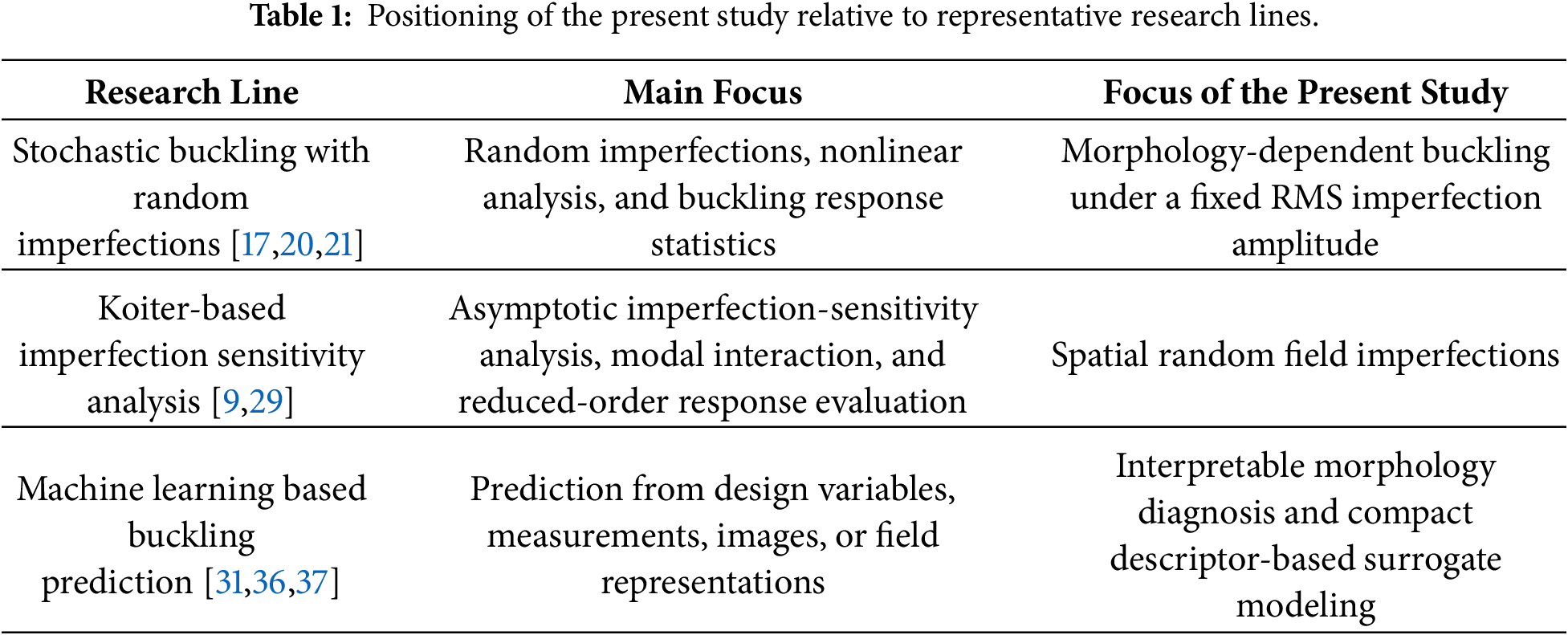
The present work uses machine learning as a tool for interpretable analysis and surrogate modeling to relate random-imperfection morphology to stochastic buckling resistance. RMS-normalized Gaussian imperfection fields with different correlation lengths are evaluated through nonlinear Riks analyses to construct the finite-element database. Feature diagnosis is subsequently performed to identify morphology descriptors that are most relevant to the buckling response, followed by compact surrogate modeling at the sample and group levels.
The main contributions of this study are summarized as follows:
• An RMS-normalized stochastic buckling database is constructed to examine correlation-length-induced morphology effects under a fixed global imperfection amplitude.
• A response-oriented feature diagnosis identifies the RMS edge jump as a compact descriptor of buckling-relevant local roughness.
• Descriptor-based surrogate models are established for efficient sample-level prediction and group-level statistical trend assessment.
The remainder of this paper is organized as follows. Section 2 introduces the geodesic random imperfection model with circumferential periodicity and the corresponding Gaussian random field generation procedure. Section 3 describes the finite-element cylindrical shell model, the stochastic imperfection database, and the nonlinear Riks analysis used to extract the critical load factors. Section 4 defines the candidate imperfection descriptors and presents the feature-diagnosis and surrogate-modeling methodology. Section 5 reports the stochastic buckling response, feature-diagnosis results, sample-level surrogate performance, and group-level statistical-response trends. Section 6 discusses the role of correlation-length-induced morphology, the interpretation of the RMS edge jump descriptor, and the limitations of the proposed framework. Section 7 concludes the paper.
2 Geodesic Random Imperfection Model with Circumferential Periodicity
2.1 Radial Geometric Imperfection of Cylindrical Shell
As shown in Fig. 1, consider a thin cylindrical shell with radius
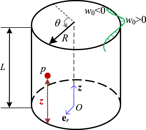
Figure 1: Radial imperfection of the cylindrical shell.
The geometric imperfection is introduced as a radial perturbation of the cylindrical middle surface. Let
where
2.2 Geodesic Distance with Circumferential Periodicity
For a cylindrical shell, the circumferential direction is periodic. As shown in Fig. 2, by unfolding the cylindrical surface into a rectangle with periodic boundary treatment in the circumferential direction, the shortest surface distance between two points
where
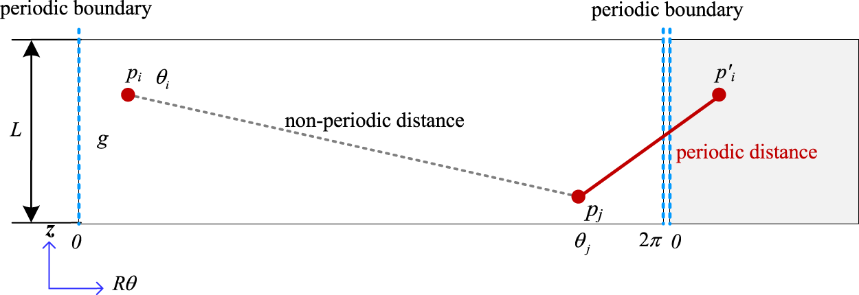
Figure 2: Geodesic distance on the unwrapped cylindrical surface with circumferential periodicity.
This distance is referred to as the geodesic distance, representing the intrinsic shortest-path distance along the cylindrical surface. The periodic treatment accounts only for the circumferential topology of the closed cylinder and prevents an artificial discontinuity at the seam of the unwrapped surface. It does not impose a periodic waveform or prescribed geometric shape on individual imperfection realizations.
For a finite element mesh with
The matrix is used to construct the covariance matrix of the random imperfection field.
2.3 Geodesic Random Field Generation with Circumferential Periodicity
The imperfection field is modeled as a zero-mean Gaussian random field,
Let
In this study, the squared-exponential covariance function is adopted:
where
The covariance matrix is then decomposed as
where
where
in which
The generated imperfection field is then scaled to a normalized imperfection amplitude as follows
where
Finally, the scaled imperfection amplitudes are applied to the nodal coordinates in the radial direction:
The prescribed correlation lengths and RMS amplitude define a controlled numerical morphology space rather than a manufacturing specific imperfection model. Application to manufactured shells therefore requires calibration of the covariance structure and imperfection amplitude from measured surface data.
3 Nonlinear Stochastic Buckling Analysis
3.1 Buckling Analysis Procedure of Finite Element Cylindrical Shell Model
The cylindrical shell model considered in this study is based on an experimental cylindrical shell reported in Ref. [20], as shown in Fig. 3. The shell has a radius of
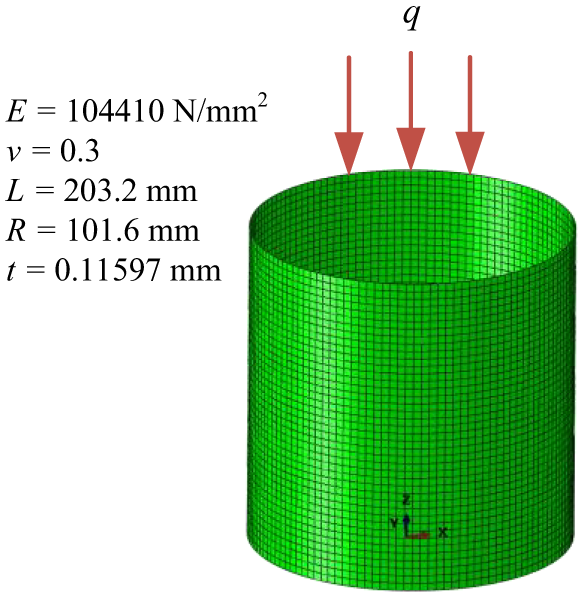
Figure 3: Finite-element model of the cylindrical shell.
The same finite element model settings were used for all imperfect shells, with only the nodal coordinates modified according to the prescribed imperfection field. For each imperfect cylindrical shell model, a geometrically nonlinear buckling analysis was performed in Abaqus 2022 using the Static, Riks procedure with NLGEOM=ON. The maximum number of increments was set to 200. The initial arc-length increment, total arc-length scale factor, minimum arc-length increment, and maximum arc-length increment were set to
The critical load factor,
3.2 Random Imperfection Database
Using the geodesic random field generation procedure described in Section 2.3, a stochastic imperfection database was constructed for the cylindrical shell. In the present parametric study, the correlation length
Eight normalized correlation lengths,
For each prescribed value of
For each value of
Fig. 4 shows representative RMS-normalized imperfection fields for selected values of
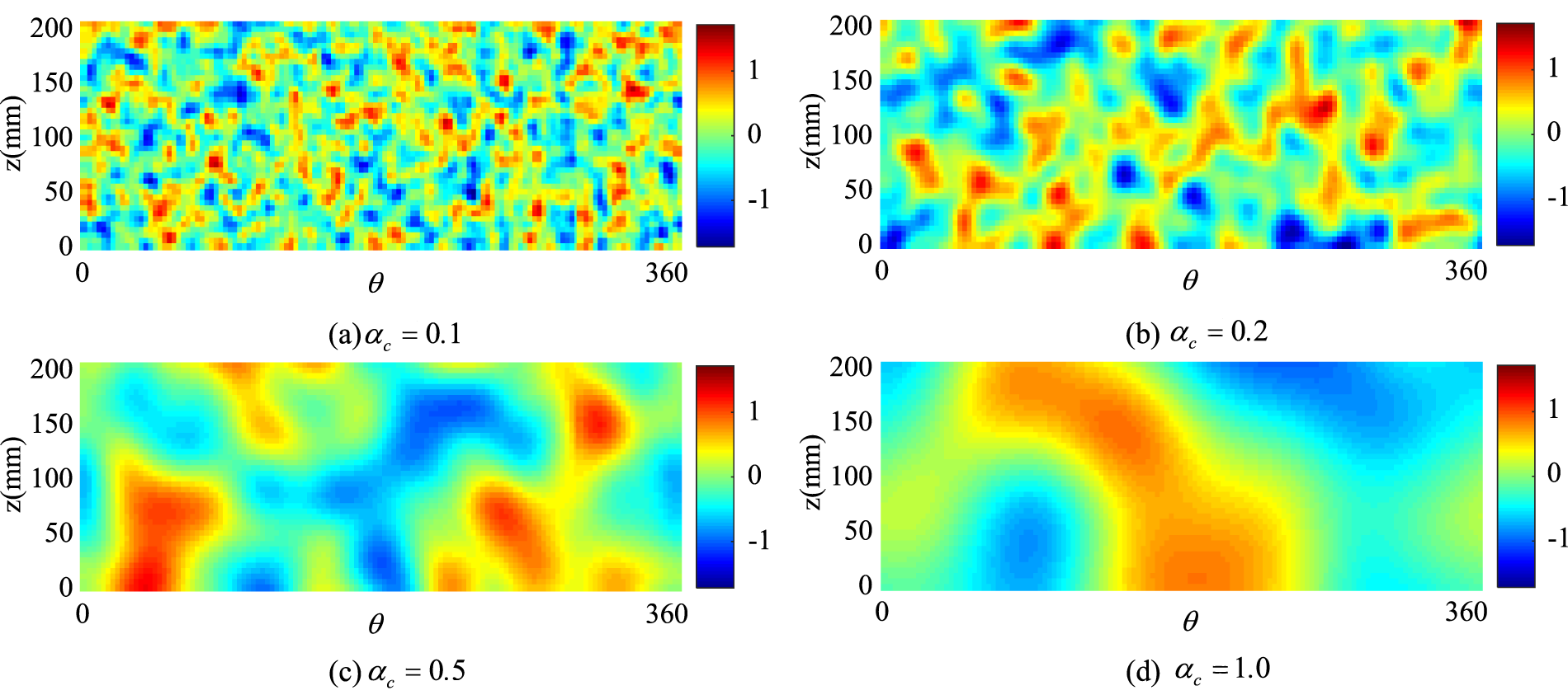
Figure 4: Representative random imperfection fields at different correlation lengths with a common RMS amplitude of
3.3 Mesh Sensitivity and Statistical Adequacy Assessment
The shortest prescribed correlation length,
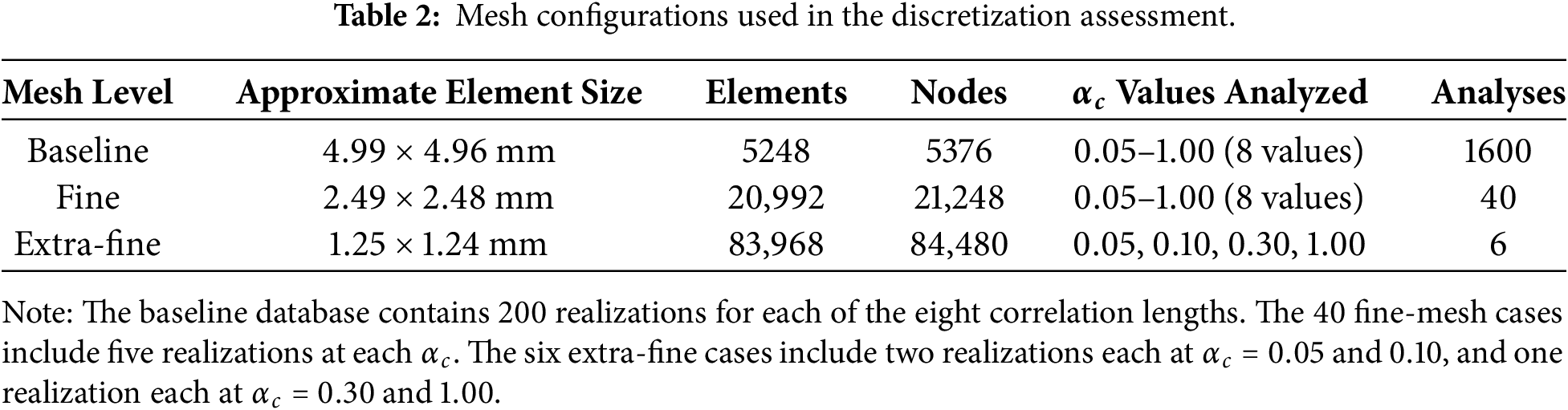
Five realizations were selected at each of the eight correlation lengths, yielding 40 paired baseline–fine comparisons. Six representative realizations were additionally analyzed using the extra-fine mesh, including two cases each at
The statistical adequacy of the 200 realizations adopted at each correlation length was further examined through repeated subsampling. Sample sizes of
4 Candidate Imperfection Descriptors and Surrogate-Modeling Methodology
4.1 Characterization of Candidate Imperfection Descriptors
The random imperfection field generated in Section 3.2 is represented by the nodal imperfection vector
The candidate descriptors considered in this study are summarized in Table 3. For the
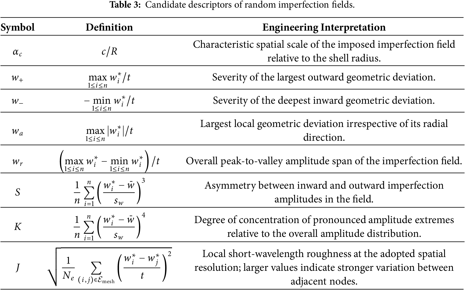
These descriptors cover four aspects of the imperfection field: the prescribed spatial scale through
Because
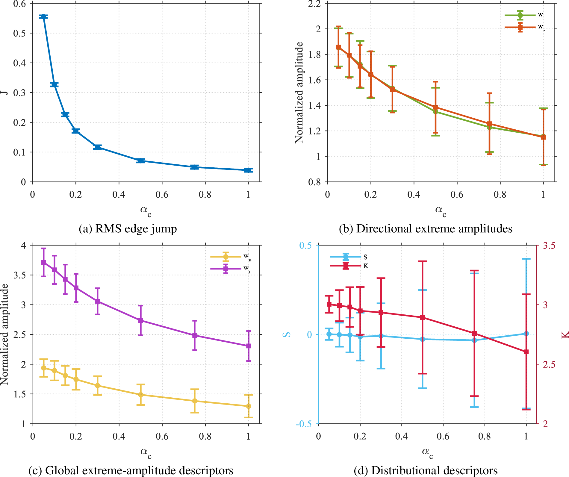
Figure 5: Variation of candidate imperfection descriptors with the prescribed normalized correlation length
Because
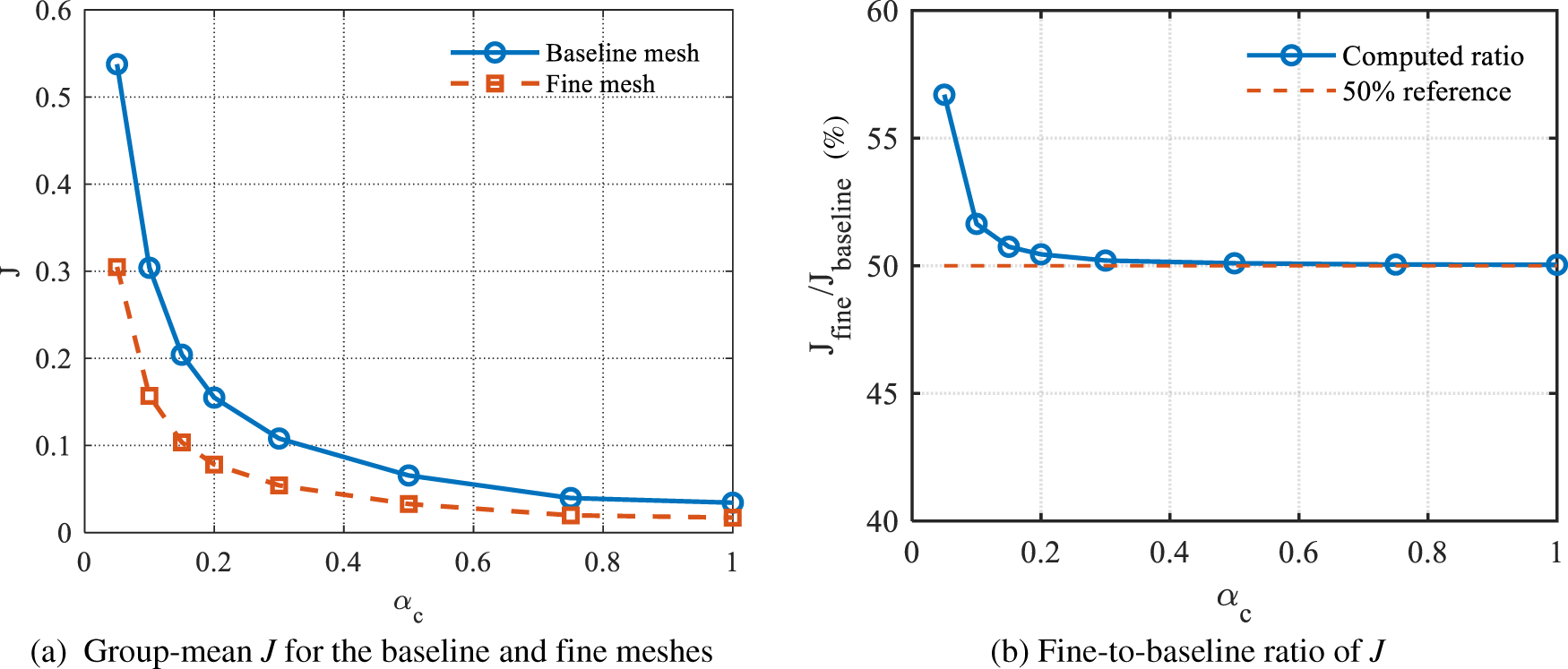
Figure 6: Resolution dependence of the RMS edge jump.
The candidate descriptors may also contain redundant information because several of them describe related aspects of the same imperfection field. For example, the amplitude-based descriptors characterize different forms of extreme-amplitude information, whereas other descriptors describe distributional shape or local variation. The correlations among the candidate descriptors are therefore examined in Fig. 7. This correlation matrix provides a preliminary view of descriptor redundancy and supports the interpretation of the subsequent feature-diagnosis and surrogate-modeling results.
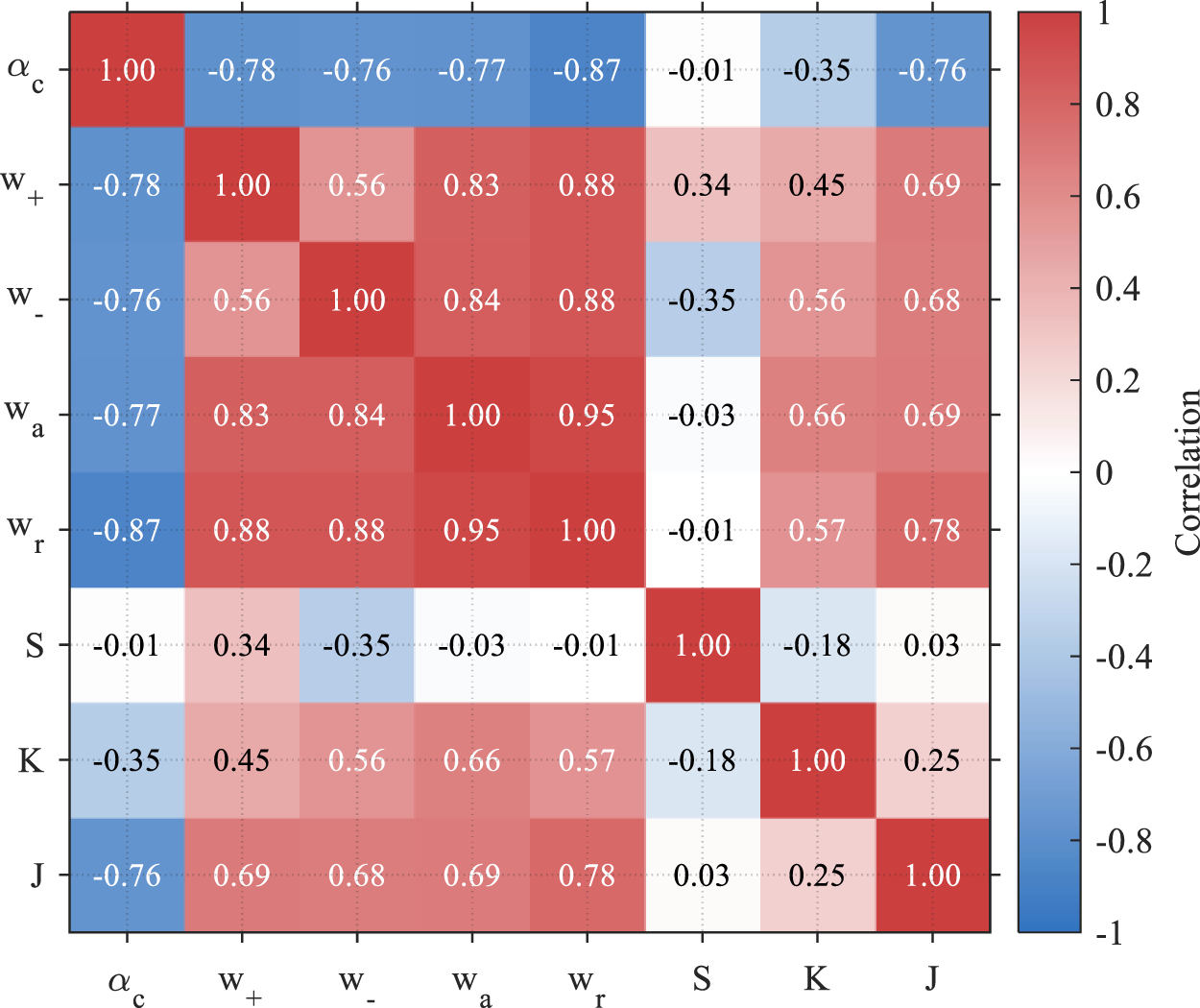
Figure 7: Correlation matrix among the candidate imperfection descriptors.
4.2 Learning Tasks and Surrogate Models
After the nonlinear Riks analyses described in Section 3.1, each random imperfection sample is associated with a critical load factor
where
Two learning tasks are considered based on this database:
here,
For sample-level prediction, five commonly used nonlinear regression algorithms were considered: bagged regression trees (BT), random forest (RF), least-squares boosting (LSBoost), support vector regression (SVR), and Gaussian process regression (GPR). The BT and RF models each used 200 regression trees trained by bootstrap resampling; BT considered all available predictors at each split, whereas RF used random predictor subsampling. LSBoost used 200 regression trees with a learning rate of 0.05. SVR used a Gaussian kernel with a kernel scale of 1, a box constraint of 1, and an epsilon-insensitive margin of 0.01. GPR used a constant basis function and an automatic-relevance-determination squared-exponential kernel with exact fitting and prediction. Predictor standardization was applied to SVR and GPR using training-set statistics only.
For group-level trend approximation, GPR was adopted, with a separate regression model established for each response statistic. The group-level input was constructed from either the prescribed generation parameter or a group summary of a candidate imperfection descriptor.
The feature-diagnosis step examines the response relevance of the candidate variables before surrogate validation. A one-way variance decomposition with respect to the
The diagnosis then consists of three complementary analyses. First, single-descriptor screening is performed using each component of
Permutation feature importance was evaluated using a bagged-tree surrogate trained with the morphology-descriptor set
Two validation protocols are used for sample-level surrogate modeling. The first applies a stratified 80%/20% holdout to the complete 1600-sample database using a fixed MATLAB random seed of 1, with 160 training and 40 test samples from each
Leave-one-group-out validation is used for the group-level statistical response trend approximation, in which one correlation length group is excluded from training and then predicted by the group-level trend approximation model. In each round, seven groups are used for fitting and the remaining group for validation, with all eight groups serving once as the held-out group. The predicted and Riks-derived values from the eight held-out groups are then compared using
The overall analysis workflow, including feature diagnosis, sample-level prediction, group-level trend approximation, and the corresponding validation procedures, is summarized in Fig. 8.
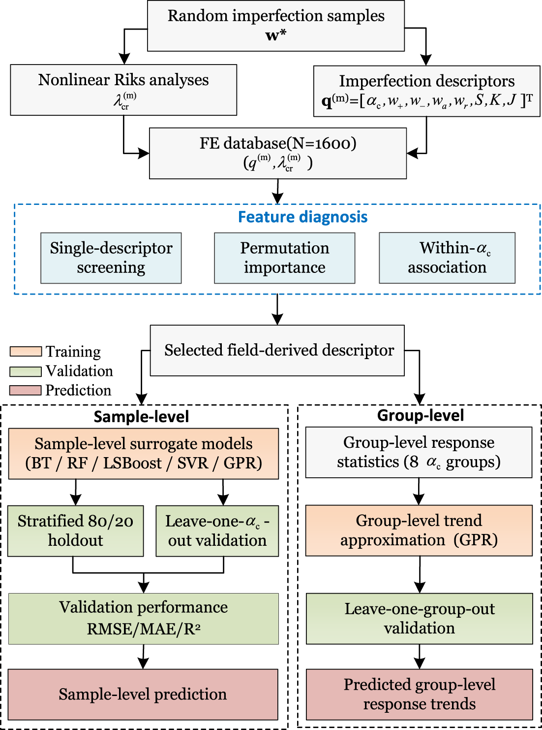
Figure 8: Workflow of feature diagnosis and surrogate-assisted stochastic buckling assessment.
5.1 Correlation-Length-Dependent Buckling Response and Robustness
Fig. 9 shows the distribution of the critical load factors for all random imperfection samples in each
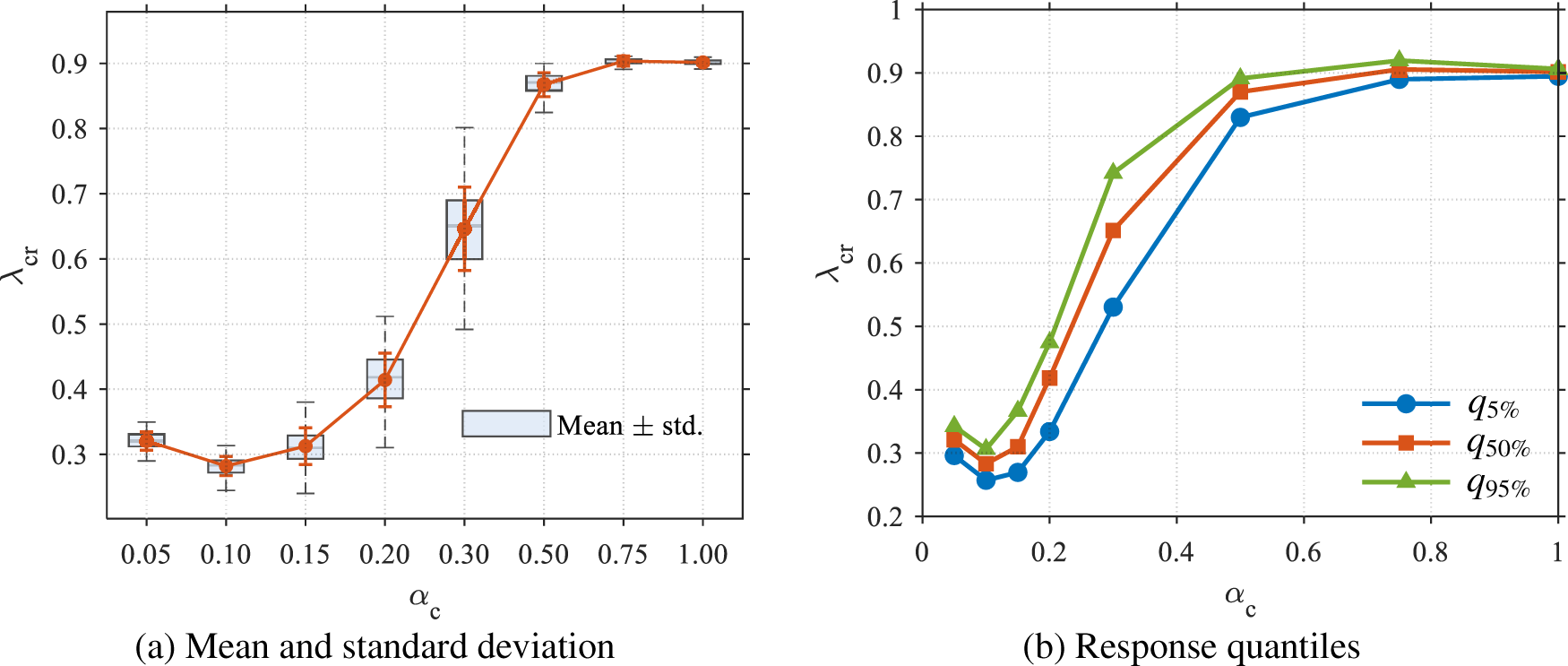
Figure 9: Distribution of
As shown in Fig. 9a, a clear but non-monotonic dependence of
The response quantiles in Fig. 9b show a consistent overall trend, remaining low at short correlation lengths, increasing rapidly over the intermediate range, and approaching a high and relatively stable level for
The mesh-sensitivity results are presented in Fig. 10. Mesh refinement changed the absolute values of
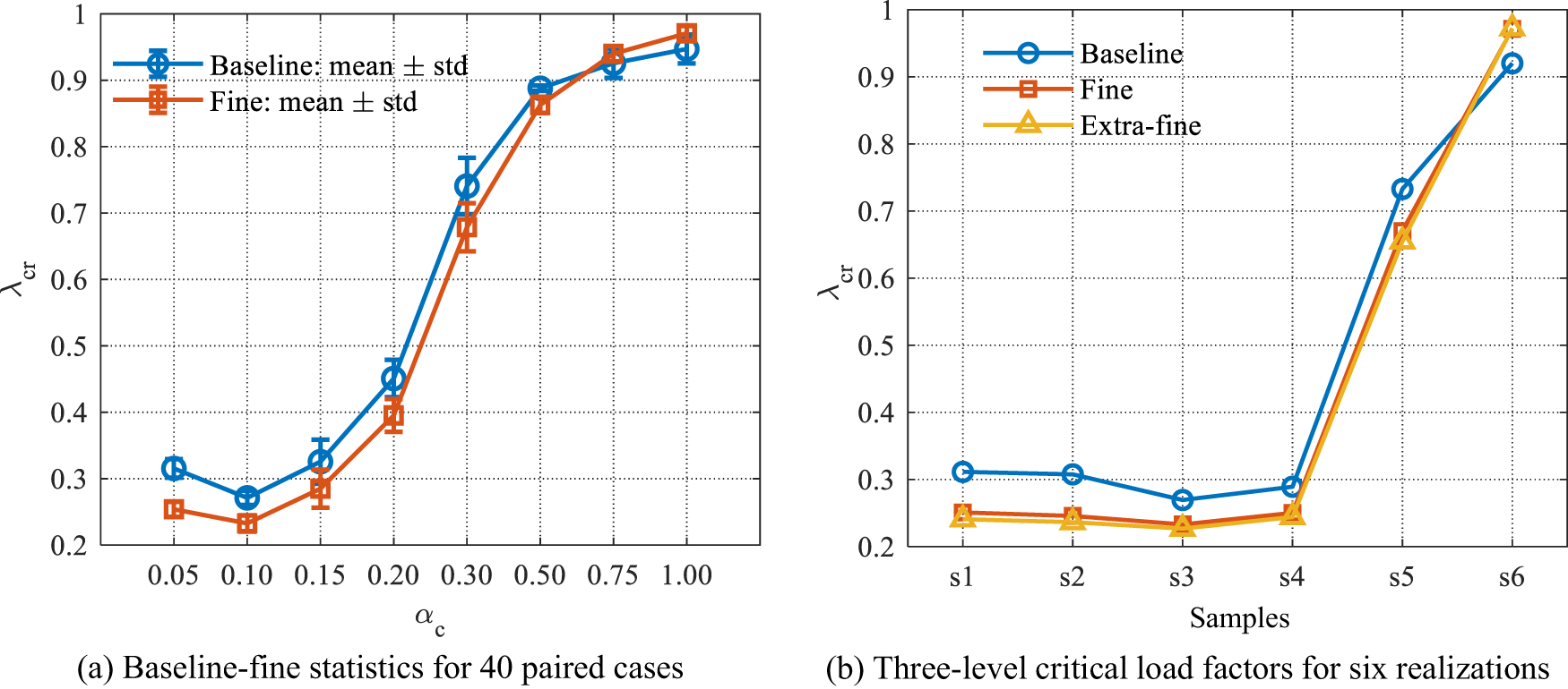
Figure 10: Mesh-sensitivity assessment of
The statistical adequacy of the database is assessed in Fig. 11 using the repeated subsampling procedure described in Section 3.3. At
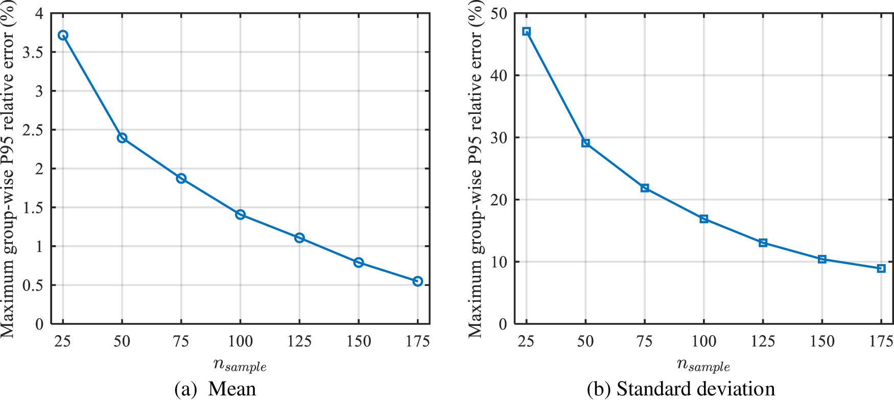
Figure 11: Subsample-based stability of the mean and standard deviation of
5.2 Machine-learning Feature Diagnosis
The results in Section 5.1 show a strong dependence of the buckling response on the prescribed normalized correlation length. A one-way variance decomposition further shows that
The response relevance of the candidate descriptors is evaluated using the procedures defined in Section 4.3. Fig. 12a shows that
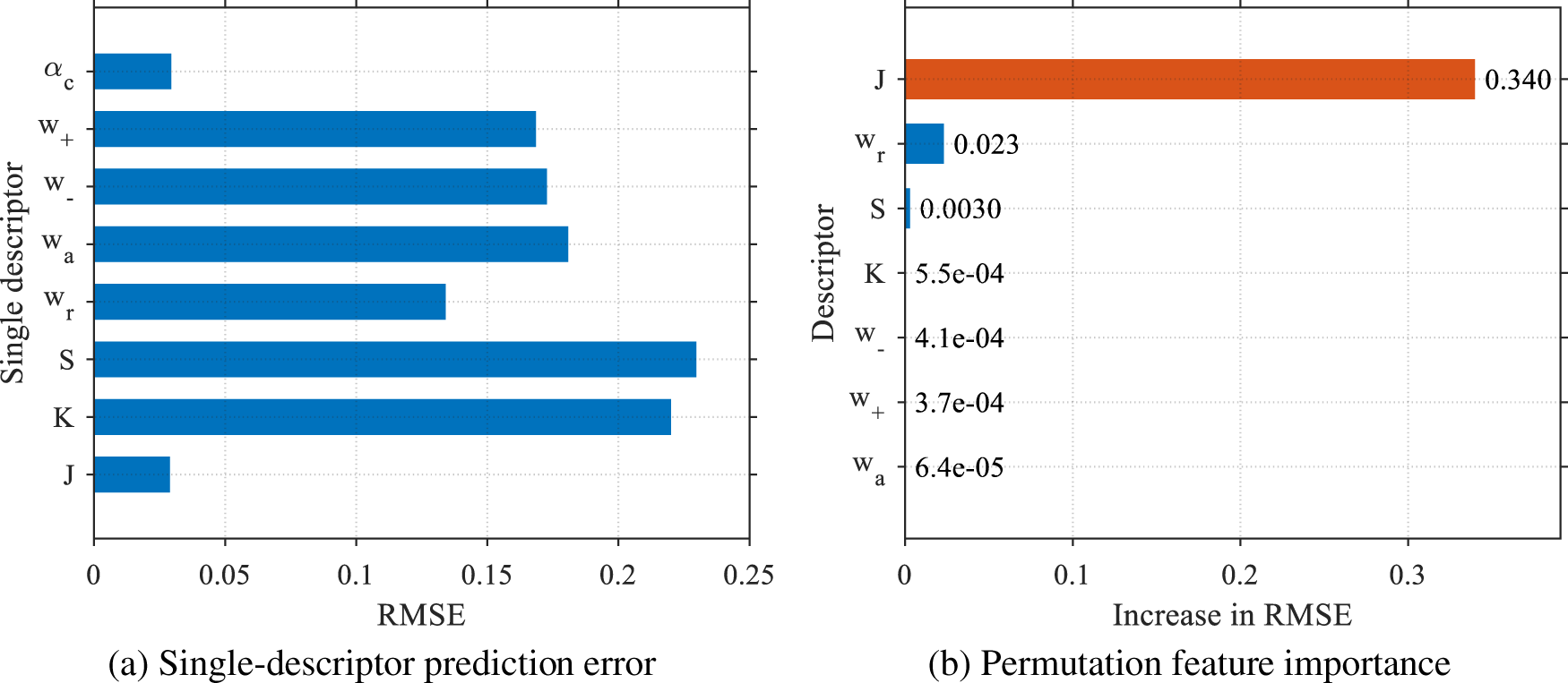
Figure 12: Predictive relevance of the candidate imperfection descriptors.
While Fig. 12 identifies
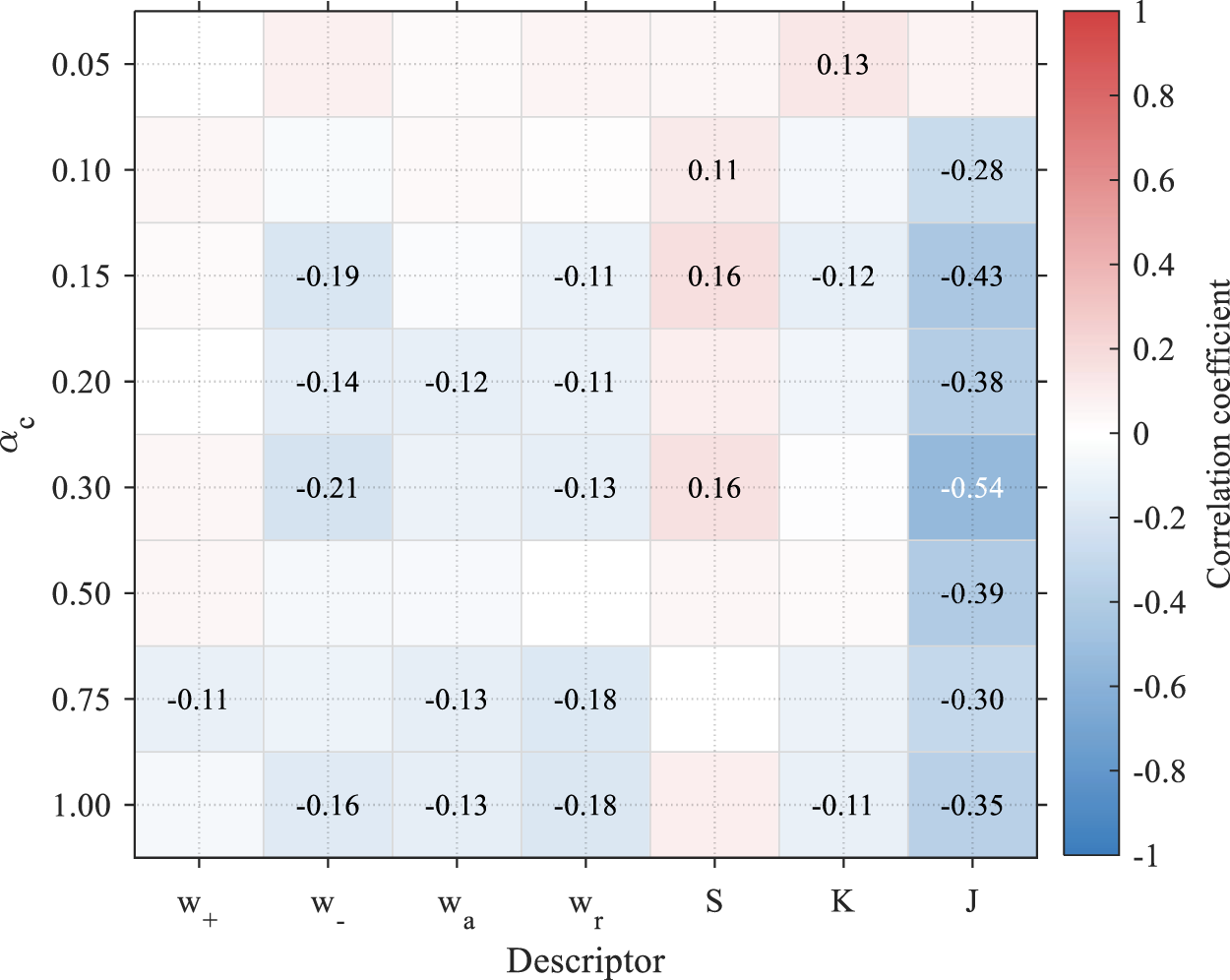
Figure 13: Within-
5.3 Sample-Level Surrogate Modeling of Critical Load Factors
Based on the feature-diagnosis results in Section 5.2, three compact input configurations are compared for sample-level prediction of
As summarized in Table 4, all three input configurations achieve similarly high accuracy under the stratified holdout, whereas clearer differences emerge under leave-one-
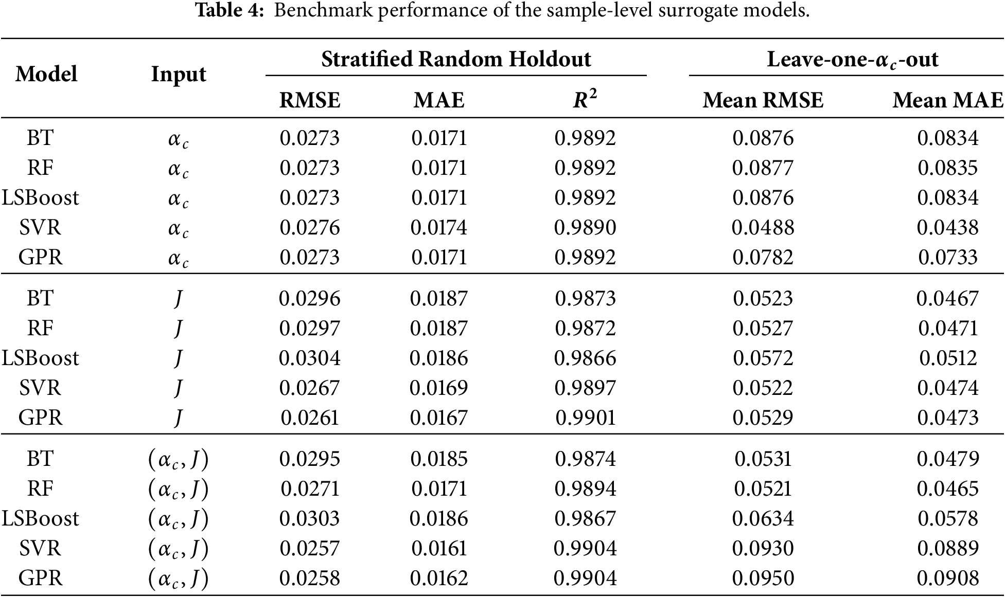
Among the
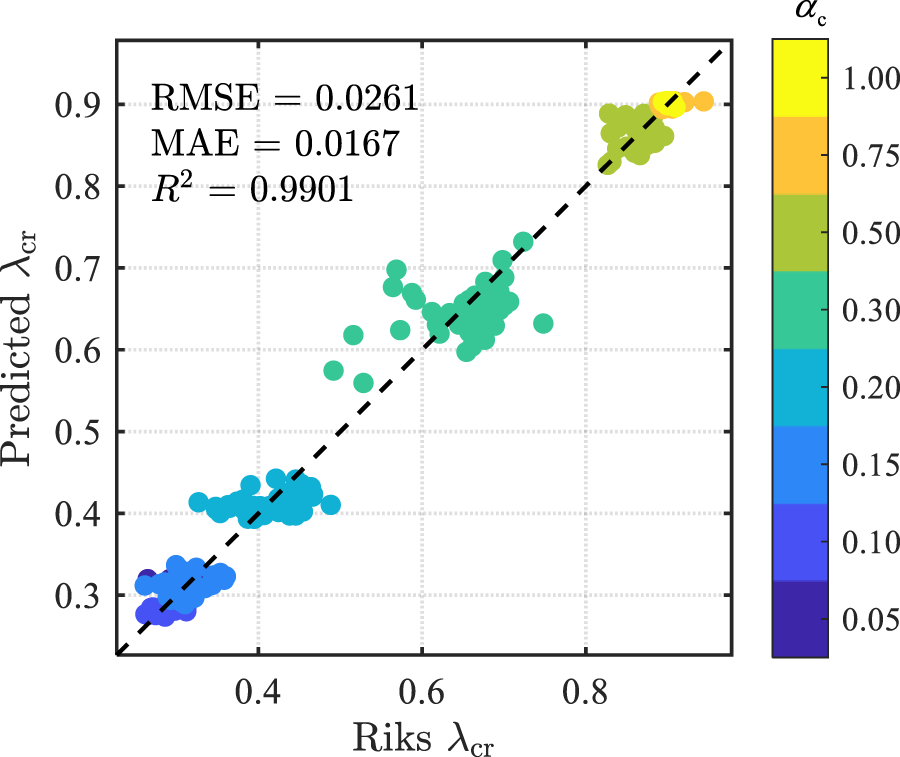
Figure 14: Predicted vs. Riks
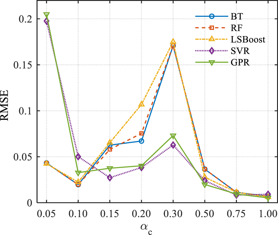
Figure 15: Leave-one-
Table 5 further examines the variation among held-out groups for the three GPR input configurations. The
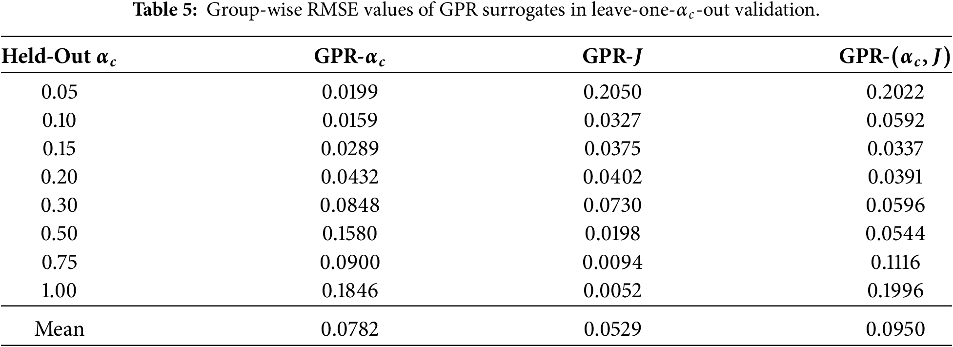
These group-wise results also show that neither
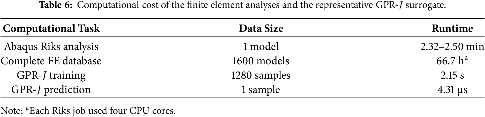
Table 6 compares the computational cost of the finite element analyses and the representative GPR-
5.4 Group-Level Statistical-Response Trend Representation
The sample-level analysis is further complemented by a group-level representation of the mean, standard deviation, and selected quantiles of
Fig. 16a,b compare the Riks-derived statistics with the corresponding group-level trend representations. Both
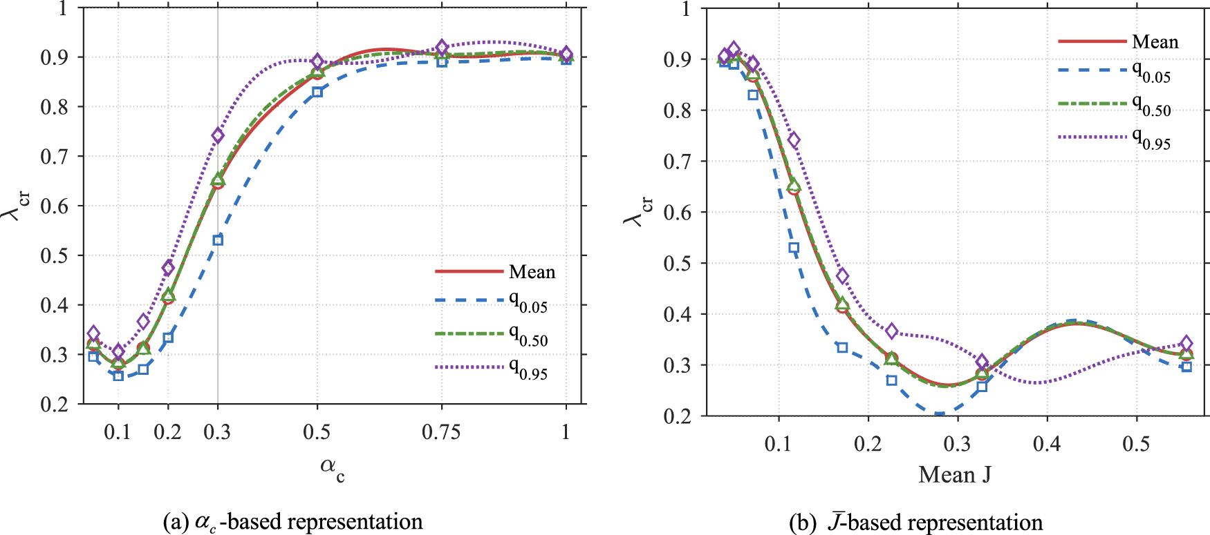
Figure 16: Group-level statistics of
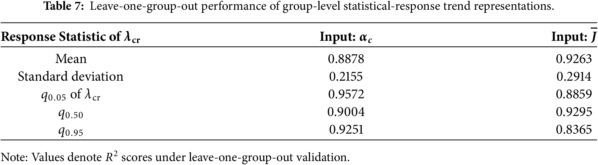
Table 7 shows that the mean and quantile trends are represented more accurately than the standard deviation. The
6.1 Mechanical Interpretation of the Unfavorable Morphology Scale
The non-monotonic response provides insight into the role of imperfection morphology beyond local roughness alone. The lowest mean critical load factor occurs at
6.2 Interpretation and Practical Role of the Morphology Descriptors
The RMS edge jump
The limited predictive relevance of the amplitude-based descriptors
The practical role of
6.3 Applicability and Limitations
The present results are obtained for a cylindrical shell with
Because both
The present database represents a controlled stochastic morphology study rather than a manufacturing specific probabilistic model, because the random field parameters were not calibrated from measured imperfection surveys. Application to manufactured shells would require measured imperfection fields to establish the relevant amplitude and spatial correlation characteristics and to evaluate the morphology descriptors at a defined resolution. Such data would also be needed to assess the transferability of
This study developed a machine-learning-assisted framework for stochastic buckling assessment of cylindrical shells with random geometric imperfections. Geometric random fields with different normalized correlation lengths were generated, scaled to the same RMS imperfection amplitude, and introduced into nonlinear Riks analyses. Based on feature diagnosis, sample-level surrogate modeling, and statistical trend assessment, the following conclusions can be drawn.
• Under the common RMS imperfection amplitude, the dominant variation of the buckling response in the present database is associated with correlation-length-induced changes in imperfection morphology, with between-
• The influence of correlation length on buckling resistance is non-monotonic. The lowest mean critical load factor does not occur at the shortest correlation length, and the largest response scatter appears in the intermediate range. Mesh refinement preserves the principal non-monotonic trend and the low-resistance regime, although the absolute critical load factors remain mesh sensitive.
• The RMS edge jump
• Compact inputs based on
The present conclusions are restricted to the investigated shell configuration, loading condition, RMS imperfection amplitude, stochastic imperfection model, and spatial resolution, and the resulting surrogates should therefore be regarded as database-dependent response approximations rather than universal buckling predictors. Future work should assess the framework against measured imperfection fields, calibrate the morphology–response relation for manufactured shells, and extend the analysis to broader structural configurations, imperfection amplitudes, and more complex non-Gaussian or localized imperfection patterns.
Acknowledgement: None.
Funding Statement: This research was funded by National Natural Science Foundation of China (grant numbers 52508233, 52578606), the Zhejiang Provincial Natural Science Foundation (grant number LQN26E080052), the visiting scholar funding of the State Key Laboratory of Disaster Reduction in Civil Engineering (grant number SLDRCE25-F-10), and the Alexander von Humboldt Foundation of Germany.
Author Contributions: The authors confirm contribution to the paper as follows: conceptualization, methodology, software, validation, formal analysis, investigation, writing—original draft preparation, funding acquisition, Yan-Ping Liang; writing—review and editing, supervision, funding acquisition, Zhiqiang Wan. All authors reviewed and approved the final version of the manuscript.
Availability of Data and Materials: Data available on request from the authors.
Ethics Approval: Not applicable.
Conflicts of Interest: The authors declare no conflicts of interest.
References
1. Lorenz R. Achsensymmetrische verzerrungen in dünnwandigen hohlzylindern. Z Ver Dtsch Ing. 1908;52(431706–13. (In German). [Google Scholar]
2. Timoshenko SP. Einige stabilitätsprobleme der elastizitätstheorie. Zeitschrift Für Mathematik Und Physik. 1910;58(4):337–85. (In German). doi:10.1002/zamm.19220020408. [Google Scholar] [CrossRef]
3. Wilson WM, Newmark NM. The strength of thin cylindrical shells as columns. In: Selected papers by Nathan M. Newmark: civil engineering classics. Reston, VA, USA: ASCE; 1933. p. 1–42. [Google Scholar]
4. Arbocz J, Babcock CD Jr. Experimental investigation of the effect of general imperfections on the buckling of cylindrical shells. Washington, DC, USA: NASA; 1968. [Google Scholar]
5. NASA/SP-8007-2020/REV 2. Buckling of thin-walled circular cylinders. Hampton, VA, USA: NASA Langley Research Center; 2020. [Google Scholar]
6. Sebek R. Imperfection surveys and data reduction of ARIANE interstages I/II and II/III [Ir thesis]. Delft, The Netherlands: Delft University of Technology; 1981. [Google Scholar]
7. Vamsi Krishna G, Narayanamurthy V, Viswanath C. Buckling behaviour of FRP strengthened cylindrical metallic shells with cut-outs. Compos Struct. 2022;300(4):116176. doi:10.1016/j.compstruct.2022.116176. [Google Scholar] [CrossRef]
8. Castro SG, Almeida JHS Jr, St-Pierre L, Wang Z. Measuring geometric imperfections of variable–angle filament–wound cylinders with a simple digital image correlation setup. Compos Struct. 2021;276(8):114497. doi:10.1016/j.compstruct.2021.114497. [Google Scholar] [CrossRef]
9. Koiter W. The effect of axisymmetric imperfections on the buckling of cylindrical shells under axial compression. Mechanics. 1963:265–79. doi:10.1090/qam/99838. [Google Scholar] [CrossRef]
10. Catellani G, Pellicano F, Dall’Asta D, Amabili M. Parametric instability of a circular cylindrical shell with geometric imperfections. Comput Struct. 2004;82(31–32):2635–45. doi:10.1016/j.compstruc.2004.07.006. [Google Scholar] [CrossRef]
11. Lauterbach S, Fina M, Wagner W. Influence of stochastic geometric imperfections on the load-carrying behaviour of thin-walled structures using constrained random fields. Comput Mech. 2018;62(5):1107–25. doi:10.1007/s00466-018-1554-0. [Google Scholar] [CrossRef]
12. Chen G, Zhang H, Rasmussen KJ, Fan F. Modeling geometric imperfections for reticulated shell structures using random field theory. Eng Struct. 2016;126(46):481–9. doi:10.1016/j.engstruct.2016.08.008. [Google Scholar] [CrossRef]
13. Fina M, Weber P, Wagner W. Polymorphic uncertainty modeling for the simulation of geometric imperfections in probabilistic design of cylindrical shells. Struct Saf. 2020;82(6):101894. doi:10.1016/j.strusafe.2019.101894. [Google Scholar] [CrossRef]
14. Shinozuka M, Deodatis G. Simulation of multi-dimensional Gaussian stochastic fields by spectral representation. Appl Mech Rev. 1996;49(1):29–53. doi:10.1115/1.3101883. [Google Scholar] [CrossRef]
15. Phoon K, Huang S, Quek S. Simulation of second-order processes using Karhunen–Loeve expansion. Comput Struct. 2002;80(12):1049–60. doi:10.1016/s0045-7949(02)00064-0. [Google Scholar] [CrossRef]
16. Chen J, He J, Ren X, Li J. Stochastic harmonic function representation of random fields for material properties of structures. J Eng Mech. 2018;144(7):04018049. doi:10.1061/(asce)em.1943-7889.0001469. [Google Scholar] [CrossRef]
17. Schenk C, Schuëller G. Buckling analysis of cylindrical shells with random geometric imperfections. Int J Non Linear Mech. 2003;38(7):1119–32. doi:10.1016/s0020-7462(02)00057-4. [Google Scholar] [CrossRef]
18. Papadopoulos V, Papadrakakis M. The effect of material and thickness variability on the buckling load of shells with random initial imperfections. Comput Methods Appl Mech Eng. 2005;194(12–16):1405–26. doi:10.1016/j.cma.2004.01.043. [Google Scholar] [CrossRef]
19. Schenk C, Schuëller G. Buckling analysis of cylindrical shells with cutouts including random boundary and geometric imperfections. Comput Methods Appl Mech Eng. 2007;196(35–36):3424–34. doi:10.1016/j.cma.2007.03.014. [Google Scholar] [CrossRef]
20. Papadopoulos V, Stefanou G, Papadrakakis M. Buckling analysis of imperfect shells with stochastic non-Gaussian material and thickness properties. Int J Solids Struct. 2009;46(14–15):2800–8. doi:10.1016/j.ijsolstr.2009.03.006. [Google Scholar] [CrossRef]
21. Majumder R, Chakraborty S, Mishra SK. Reliability analysis and design of randomly imperfect thin cylindrical shells against post-critical drops. Thin Walled Struct. 2023;185(11):110576. doi:10.1016/j.tws.2023.110576. [Google Scholar] [CrossRef]
22. Scarth C, Adhikari S, Cabral PH, Silva GHC, Prado AP. Random field simulation over curved surfaces: applications to computational structural mechanics. Comput Methods Appl Mech Eng. 2019;345:283–301. [Google Scholar]
23. Feng DC, Liang YP, Ren X, Li J. Random fields representation over manifolds via isometric feature mapping-based dimension reduction. Comput Aided Civ Infrastruct Eng. 2021;37(5):593–611. doi:10.1111/mice.12752. [Google Scholar] [CrossRef]
24. Liang YP, Ren X, Feng DC. Efficient stochastic finite element analysis of irregular wall structures with inelastic random field properties over manifold. Comput Mech. 2022;69(1):95–111. doi:10.1007/s00466-021-02084-4. [Google Scholar] [CrossRef]
25. Liang YP, Feng DC, Ren X, Li J. Three-stage non-Gaussian homogeneous random field representation over manifolds. Comput Aided Civ Infrastruct Eng. 2023;38(11):1462–82. doi:10.1111/mice.12959. [Google Scholar] [CrossRef]
26. Zhang D, Chen Z, Li Y, Jiao P, Ma H, Ge P, et al. Lower-bound axial buckling load prediction for isotropic cylindrical shells using probabilistic random perturbation load approach. Thin Walled Struct. 2020;155(2):106925. doi:10.1016/j.tws.2020.106925. [Google Scholar] [CrossRef]
27. Mahidan F, Ifayefunmi O. The imperfection sensitivity of axially compressed steel conical shells-lower bound curve. Thin Walled Struct. 2021;159(2):107323. doi:10.1016/j.tws.2020.107323. [Google Scholar] [CrossRef]
28. Wagner HNR, Hühne C, Elishakoff I. Probabilistic and deterministic lower-bound design benchmarks for cylindrical shells under axial compression. Thin Walled Struct. 2020;146(79):106451. doi:10.1016/j.tws.2019.106451. [Google Scholar] [CrossRef]
29. Barbero EJ, Madeo A, Zagari G, Zinno R, Zucco G. Imperfection sensitivity analysis of composite cylindrical shells using Koiter’s method. Int J Comput Methods Eng Sci Mech. 2017;18(1):105–11. doi:10.1080/15502287.2016.1276359. [Google Scholar] [CrossRef]
30. Tahir ZR, Mandal P. Artificial neural network prediction of buckling load of thin cylindrical shells under axial compression. Eng Struct. 2017;152(4):843–55. doi:10.1016/j.engstruct.2017.09.016. [Google Scholar] [CrossRef]
31. Tahir ZuR, Mandal P, Adil MT, Naz F. Application of artificial neural network to predict buckling load of thin cylindrical shells under axial compression. Eng Struct. 2021;248(11):113221. doi:10.1016/j.engstruct.2021.113221. [Google Scholar] [CrossRef]
32. Lin X, Jiao P, Xu H, Li X, Chen Z. A machine learning-driven prediction of lower-bound buckling design load for cylindrical shells under localized axial compression. Thin Walled Struct. 2025;209:112960. doi:10.1016/j.tws.2025.112960. [Google Scholar] [CrossRef]
33. Lee HG, Sohn JM. A comparative analysis of buckling pressure prediction in composite cylindrical shells under external loads using machine learning. J Mar Sci Eng. 2024;12(12):2301. doi:10.3390/jmse12122301. [Google Scholar] [CrossRef]
34. Tao F, Liu X, Du H, Yu W. Physics-informed artificial neural network approach for axial compression buckling analysis of thin-walled cylinder. AIAA J. 2020;58(6):2737–47. doi:10.2514/1.j058765. [Google Scholar] [CrossRef]
35. Liu F, Chen H, Yang J, Wang X. Application of physics-informed machine learning methods in buckling design of axially compressed cylindrical shells. Thin Walled Struct. 2024;200(5):111963. doi:10.1016/j.tws.2024.111963. [Google Scholar] [CrossRef]
36. Hao P, Duan Y, Liu D, Yang H, Liu D, Wang B. Image-driven intelligent prediction of buckling behavior for geometrically imperfect cylindrical shells. AIAA J. 2023;61(5):2266–80. doi:10.2514/1.j062470. [Google Scholar] [CrossRef]
37. Schweizer M, Fina M, Wagner W, Kasic S, Freitag S. Artificial neural networks for random fields to predict the buckling load of geometrically imperfect structures. Comput Mech. 2025;76(1):181–204. doi:10.1007/s00466-024-02595-w. [Google Scholar] [CrossRef]
38. Wafi MG, Palar PS, Robani MD, Jusuf A, Zuhal LR, Morlier J. Revisiting cylindrical buckling under axial compression using explainable machine learning. In: Proceedings of the AIAA SCITECH, 2024 Forum; 2024 Jan 8–12; Orlando, FL, USA. [Google Scholar]
39. Zhan M, Wang H, Li Y, Wang L. Explainable machine-learning-assisted hydrostatic failure analysis of moderately thick composite cylindrical shells with ovality. Ocean Eng. 2026;357:125597. doi:10.1016/j.oceaneng.2026.125597. [Google Scholar] [CrossRef]
40. Chen H, Chen G, Yang D, Fu ZJ. Neural network-based DPIM for uncertainty quantification of imperfect cylindrical stiffened shells with multiple random parameters. Eng Anal Bound Elem. 2024;166(12):105795. doi:10.1016/j.enganabound.2024.105795. [Google Scholar] [CrossRef]
Cite This Article
 Copyright © 2026 The Author(s). Published by Tech Science Press.
This work is licensed under a Creative Commons Attribution 4.0 International License , which permits unrestricted use, distribution, and reproduction in any medium, provided the original work is properly cited.
 Downloads
 Citation Tools
