A Work Review on Clinical Laboratory Data Utilizing Machine Learning Use-Case Methodology

1  Introduction

Rheumatology is a branch of medicine that deals with diagnosing and treating rheumatic disease. Autoimmune diseases, autoinflammatory diseases, crystalline arthritis, metabolic bone diseases, etc., come under the rheumatic disease category [1]. No single blood test can quickly confirm a rheumatic disease diagnosis [2]. ANA (Antinuclear Antibody) is the standard test to identify rheumatic disease. However ANA could be positive in many conditions for an average human. The immune system produces antibodies that react with self-antigens, causing pathology, known as autoantibodies [3]. Autoantibodies cause autoimmune disease [4]. There are 13 subcategories of death in autoimmune diseases. Diabetes, multiple sclerosis, pernicious anaemia, arthritis, and lupus are the five autoimmune diseases that cause the most deaths, from most to least [5]. Regardless of gender, both males and females suffer from many arthritis diseases. Females are affected more than males because of autoimmune arthritis [6]. Though much research has been done on treating autoimmune diseases, finding biomarkers that play a significant role in identifying them is necessary. Exploring the significance of hidden biomarkers in autoimmune disease prognosis is also indispensable. Only a few research studies have been initiated in predicting autoimmune disease using patient data [7]. Discovering hidden biomarkers is the one plausible research that must be addressed from autoimmune patient data records.

A subset of artificial intelligence is ML, where the machine learns from the existing data and decides to solve the problem quickly [8]. Prediction of autoimmune diseases are done using ML algorithms [9]. The arthritis profile patient data was collected from Sri Eswari Lab, Karaikudi, Tamil Nadu, to predict autoimmune arthritis disease and identify significant and hidden biomarkers using ML algorithms.

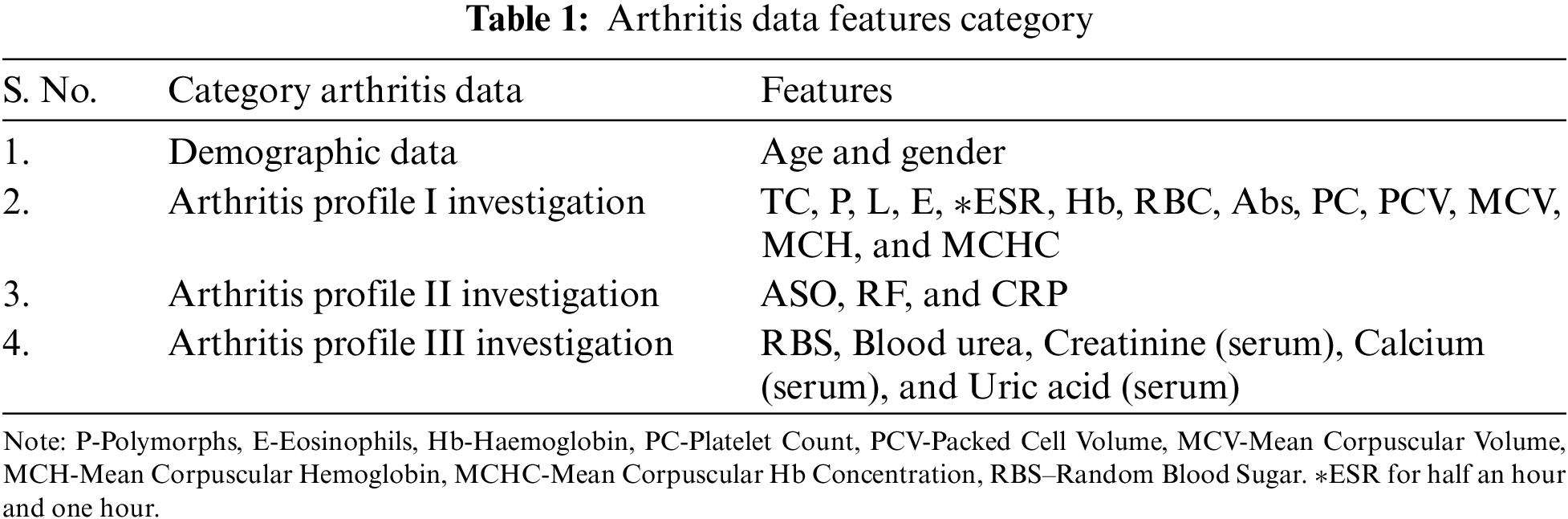
Over one year, from February 2021 to February 2022, we collected arthritis information from Sri Easwari Computerized Lab, Karaikudi, Tamil Nadu, India. The clinical laboratory provided patient details that consisted of demographic data and Arthritis Profile I investigations data, Arthritis Profile II investigations data, and Arthritis Profile III investigations data. The attributes of the arthritis data category are displayed in Table 1. We named the dataset as ‘Arthritis Profile Data’ (APD). The APD has 24 attributes and 52 data points. Except for the ‘gender’ feature, every feature in our dataset has numeric, discrete, and continuous values. ‘Gender’ and ‘RF’ are the only attributes with no mislaid data. Empty data points within the APD dataset implies each information point is missing at least one feature value [10].

Our work significantly contributes to the domain of clinical laboratory data and machine learning methodologies in the following key aspects:

•   Identifying suitable imputation techniques tailored to the APD dataset enhances data completeness.

•   Discerning the selection of a ML model well-aligned with the APD dataset characteristics.

•   Other hidden biomarkers have been recognized in addition to the well-known biomarkers.

•   It has been identified that the inherent characteristics of the dataset significantly impact the accuracy score.

•   The substantial impact of the HO method and CV fold size on model accuracy provides key methodological insights have been identified.

The remaining review comprises the following sections: The second section describes the generic methodology for ML use cases. The third section discusses acceptable ML imputation approaches for arthritis profile data, while the fourth section compares arthritis profile data with other benchmark datasets and discusses viable ML algorithms for it. Section 5 explains the conclusion of our study and recommends future work.

2  General Approach for Use Case Using ML Model

The use case exploited for our research work is to assess whether the patient is affected with autoimmune arthritis disease. Fig. 1, the flow diagram, narrates the ML model for any use case. In our scenario, the initial step is the data collection process [11]. As mentioned earlier, data were collected from a computerized lab. Next is to check whether the collected data is in the proper format to create a ML model. Since the collected information is not in the appropriate form, the next step is data preprocessing.

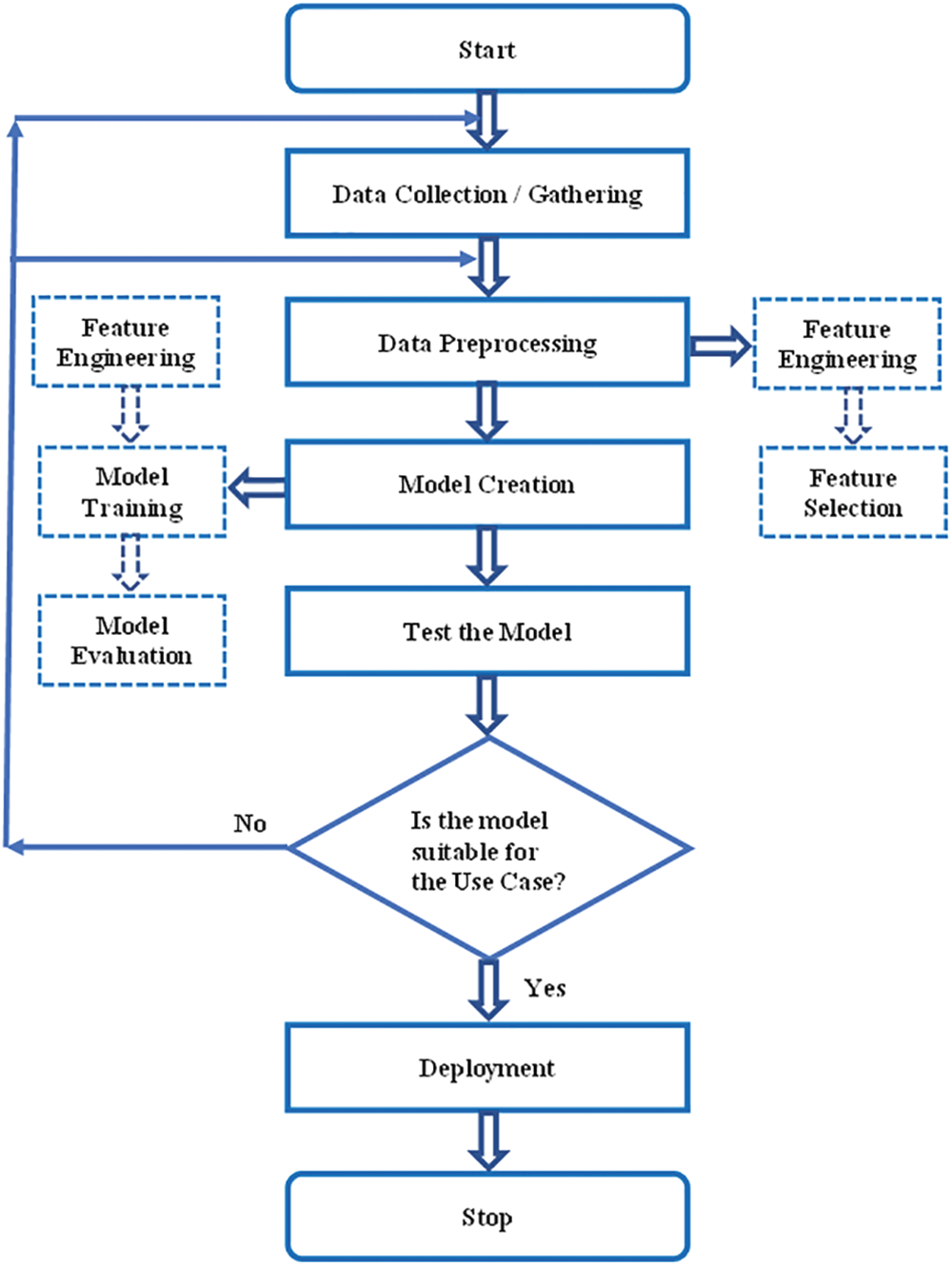
Figure 1: Flow diagram of use case using machine learning model

In the data preprocessing step, feature engineering and feature selection are performed [12]. Feature Engineering examines each feature and converts it into the proper format so it is in an acceptable input format for the ML algorithm. Handling categorical variables, handling missing values, handling imbalanced datasets, etc., are performed in feature engineering. In feature selection, certain features are removed by checking the correlation or covariance of the predictor and target variables. If the target variable is not correlated with the independent variable, that variable is suggested to be removed.

Since the APD data has missing values, it is handled using imputation techniques in our use case. Moreover, feature selection is performed to reduce the curse of dimensionality. Detailed descriptions of imputation techniques in the APD dataset will be explained in the forthcoming section. According to Fig. 1, the next step to be followed is modeling after data preprocessing.

Model creation consists of feature engineering, model training, and model evaluation. Normalization is applied to the features. Once the feature values are in the proper format, different ML as well as deep learning techniques can be applied [13]. The suitable ML algorithm for our use case is finally identified by performing model evaluation such as accuracy and confusion matrix and by following CV and hyperparameter optimization [14]. The best suitable ML model for the use case is the ML algorithm that secures the highest score. In our scenario, different HO and CV methods have obtained a suitable ML algorithm for the APD dataset. A detailed description of this study will be discussed in the forthcoming section. The trained model is tested using the test data, and its prediction accuracy is checked. If its accuracy is good, deployment can be done using web services. If not, there may be an issue in the collected data or in data preprocessing, so it is necessary to continue the same process again. The coding was done using Python which is well known for its excellent feature such as robust portability, good interpretability, and strong versatility. The computer hardware specifications used for our experiments are CPU operating at @ 2.40 and 2.42 GHz, 12 GB of memory, and 64-bit operating system.

3  Assessment of Relevant Imputation Techniques for the APD Dataset

Fig. 2 shows percentage (%) of missing feature values in the APD dataset. The mislaid value was absent in the ‘RF’ and ‘Gender’ features. The missing values in each feature were handled using ML imputation techniques. Many researchers have suggested different imputation techniques for their proposed work [15–19]. Various ML algorithms reveal different model performance and classification accuracy. In general, each incomplete dataset may vary its ML model performance depending on the different imputation techniques applied to it. Therefore, selecting a pertinent imputation technique for the incomplete record set is necessary.

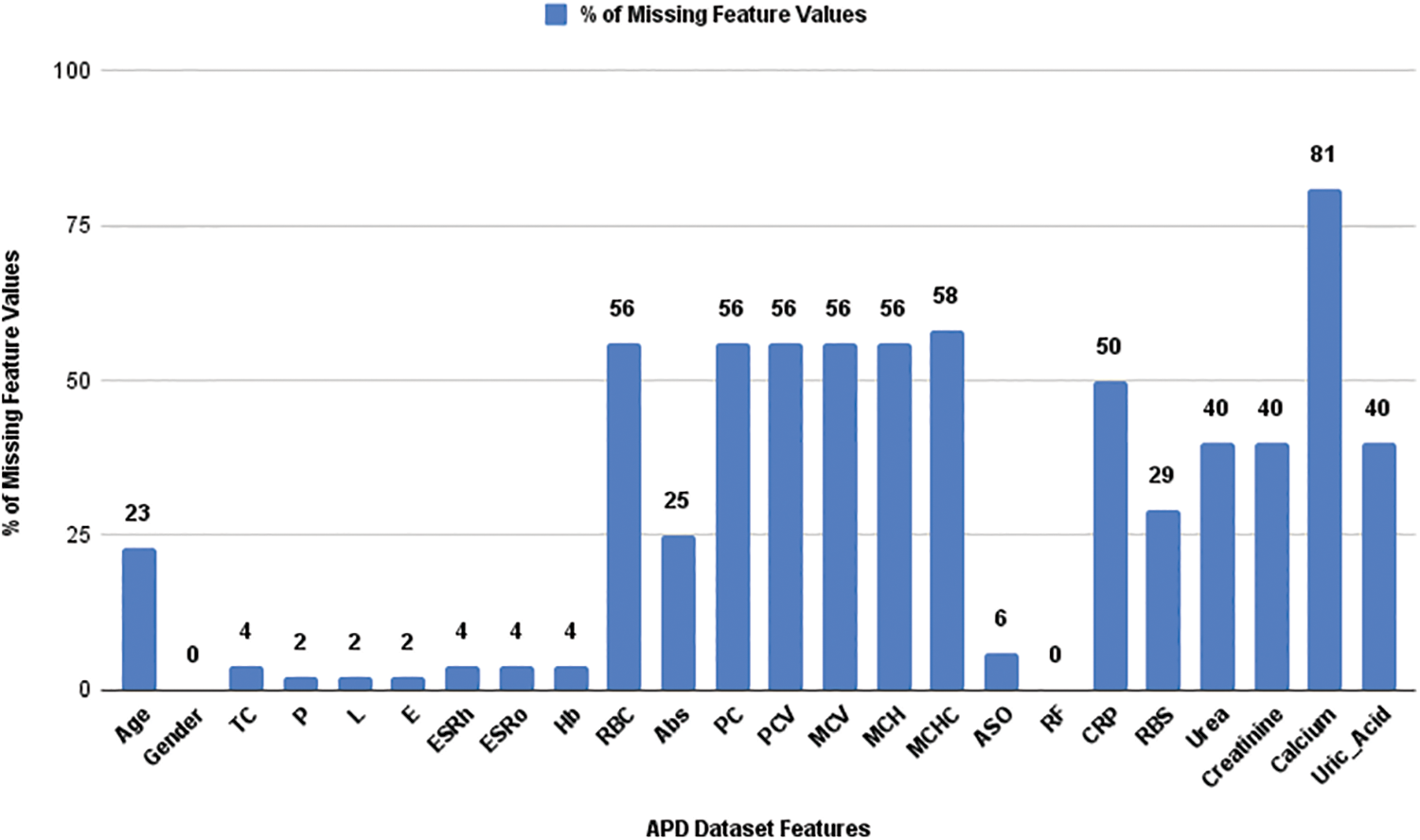
Figure 2: Percentage of missing values in the APD dataset features

ML models are commonly employed by researchers to address missing and imputed (imp) data. The findings of these studies can vary depending on several factors, including the record set domain, the type of missing categories (such as Missing Completely at Random (MCAR), Missing at Random (MAR), and Missing not at Random (MNAR)), the pattern of missingness, missingness percentage in the data sample, and the chosen imputation techniques. Further investigation into imputation techniques is consistently required as their efficacy is contingent upon multiple factors. Implementing both ML algorithms and traditional imputation techniques is possible, but discerning which method outperforms the other poses a challenge. Additionally, the assessment of imp data relies on varying metrics in accordance with the researchers investigation.

The seven imp APD datasets were generated using imputation techniques. The imputation techniques that were applied include mean, median, mode (using the first index of the mode value), random value, K-nearest neighbors (KNN), Multiple Imputation by Chained Equation (MICE), and Random Forest (RndF) imputation. Statistical parameters such as arithmetic average (mean), midpoint (median), and standard deviation (SD) were computed for the partial data sample and for all the seven complete imp information sets. By analyzing the statistical parameters, a comparison was made between the distribution of the seven imp datasets and the actual datasets. Furthermore, the DoP was assessed for each of the seven imp datasets to identify the values that closely resemble the values in the incomplete APD dataset. A higher DoP indicates a greater similarity between the imp and original values.

Selecting the most effective imputation techniques depends on the suggested proximity and residual evaluation measures. The overall process for assessing proximity involves determining the extent to which the imp values in the dataset deviate from the original values. This is done by considering statistical properties such as arithmetic average (mean), midpoint (median) and modal value. Similarly, the general procedure for evaluating residual focuses on quantifying the discrepancy between the original and imp values.

The Fig. 3 procedure depicts the appropriate imputation strategies are determined based on the DoP. The mean imp value, MICE imputer, and random forest dataset are the most effective imputation techniques when utilizing mean statistical properties. Similarly, the median imp value, random value imputer, and random forest dataset are the top three imputation procedures for median statistical properties. Furthermore, the preferred imputation approaches for SD statistical properties are the random value imputer, KNN imputer, and mode imp value.

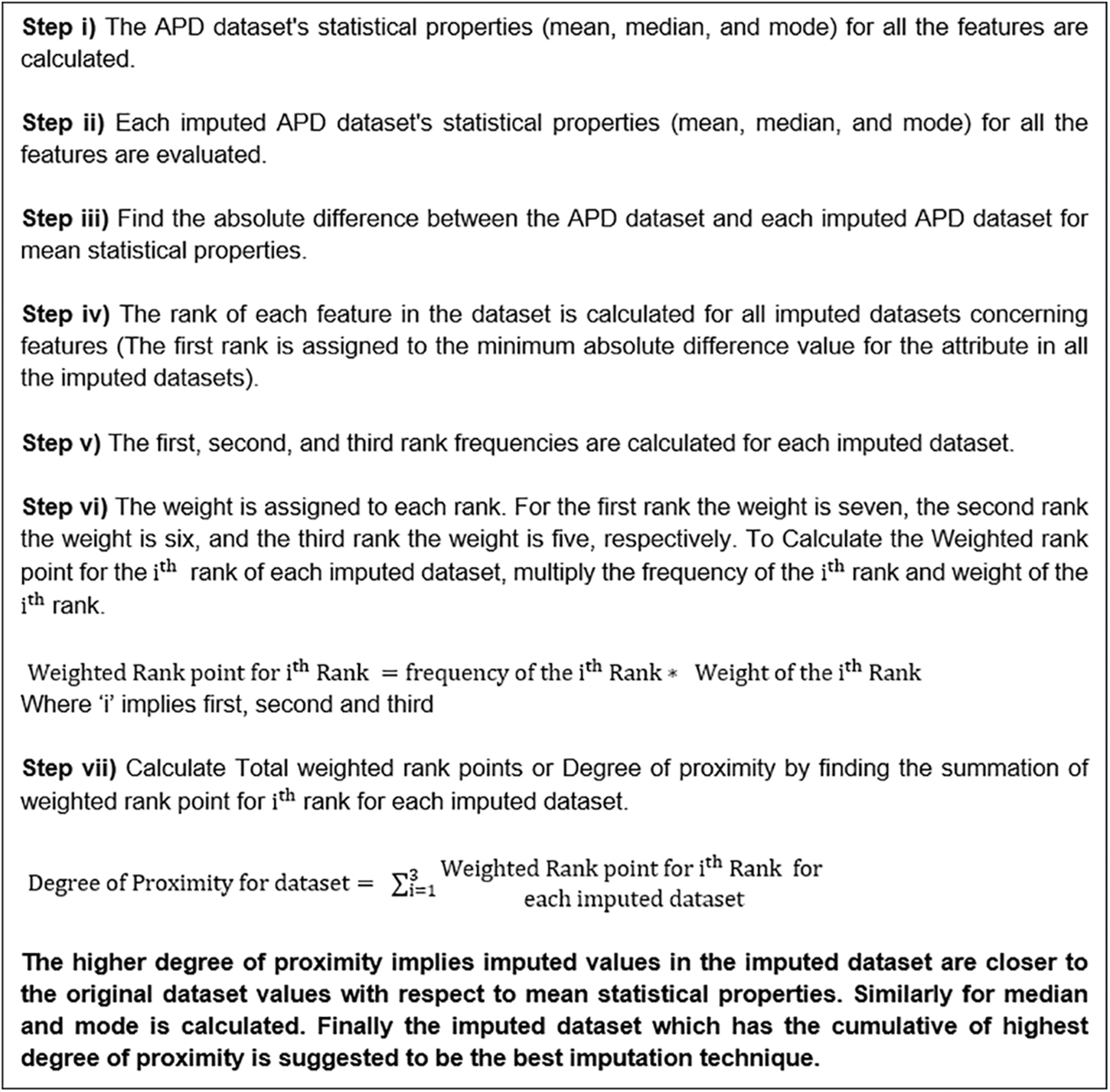
Figure 3: Generic procedure to analyze the degree of proximity in the dataset

To evaluate the imp datasets, the Imp Mean Average Error (MAEim), Imp Mean Square Error (MSEim), Imp Root Mean Square Error (RMSEim), and Imp Coefficient of determination or R-Squared (R2im) are computed between each imp dataset and the original partial APD dataset (with mislaid values substituted by zero) to each feature.

To assess the attainment of the imp dataset, we utilize three metrics: MAEim, RMSEim, and R2im. These metrics help us measure the level of residual present. Our primary objective is to determine the variance (error) between the original and imp values, as this provides insight into the performance of the imp dataset. Once we have calculated these evaluation criteria, the next step is to rank each imp dataset based on its attributes. We then apply the residual technique to each performance metric, where a higher DoR corresponds to a smaller residual in the imp dataset.

Using the method depicted in Fig. 4, the acceptable imputation strategies are identified based on the DoR. If the MAEim is zero, it indicates that the attribute contains no mislaid values. The imp dataset exhibits a reduced error when utilizing the mode imp value, median imp value, and KNN imputer, indicating higher precision. Conversely, the imp datasets produced by the RMSEim metrics, such as the mode imp value, median imp value, and MICE imputer, exhibit a larger residual, implying lower accuracy. When employing the R2im metrics, the imp datasets that demonstrate a larger residual, suggesting greater inaccuracy, are the mode, median, and random value imp.

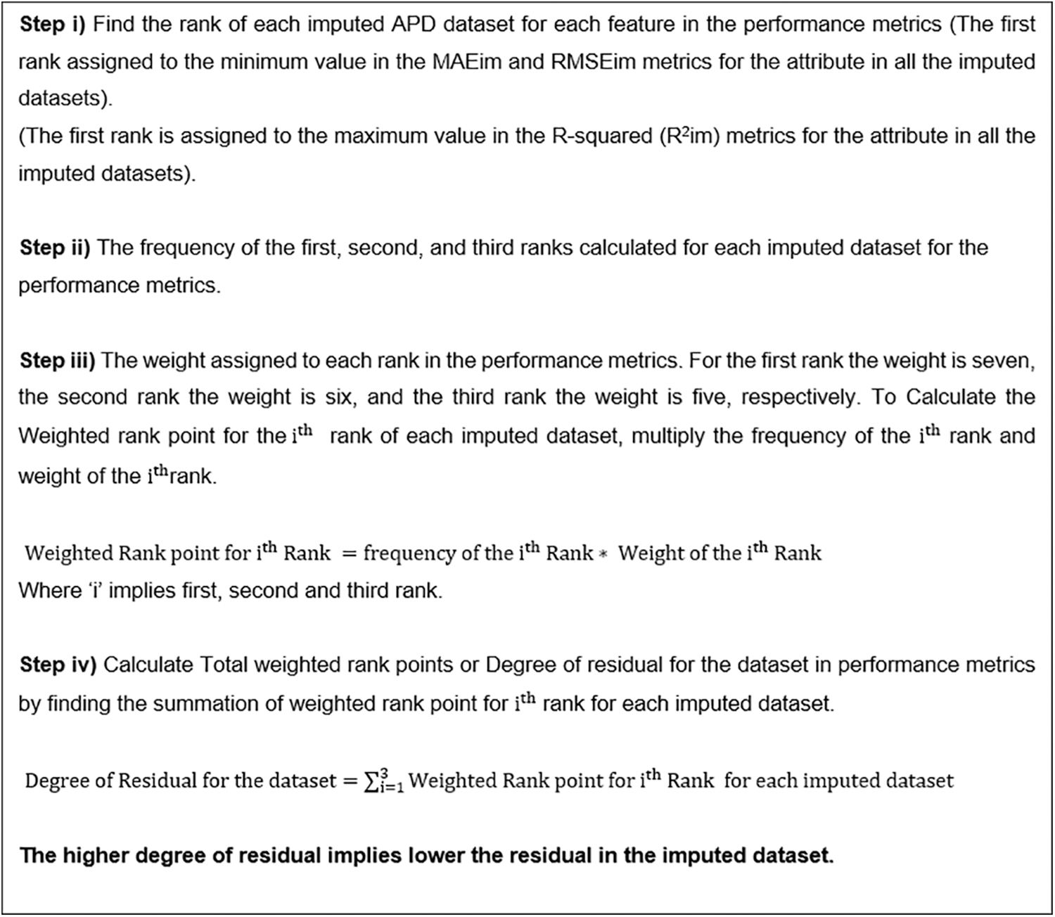
Figure 4: Generic procedure to analyze the degree of residual in the dataset

The random value imputer is the most effective in determining proximity among the seven imputation approaches. The median imp value and the MICE imputer closely follow it. Regarding the imp error, the mode imp value, median imp value, and KNN imputer have the lowest values, while the random value imputer and MICE imputer are close behind.

4  Analysis of Suitable ML Algorithm for the APD Dataset

Autoimmune arthritis illnesses, such as rheumatoid arthritis (RA), psoriatic arthritis, and juvenile arthritis, fall under the category of rheumatic diseases. Information regarding arthritis profiles was gathered from Sri Easwari Computerized Lab in Karaikudi, Tamil Nadu, India, over one year and six months, from February 2021 to August 2022. The updated APD dataset has 24 attributes and 102 data points. The dataset includes patient information for individuals with and without autoimmune arthritis disease. The subsequent study aims to assess the arthritis dataset using ML algorithms, classification techniques, and ensemble approaches to uncover hidden biomarkers. Additionally, the research aims to compare the arthritis dataset with other benchmark datasets to determine if the dataset’s characteristics impact the accuracy of the ML model.

The following benchmark disease datasets were used for comparison with the APD dataset: Wisconsin Breast Cancer (WBC) [20–22], cardiovascular disease (CVD) [23–27], Pima Indians Diabetes Mellitus (PIMA) [28–30], chronic kidney disease (CKD) [31–34] and RA dataset [35].

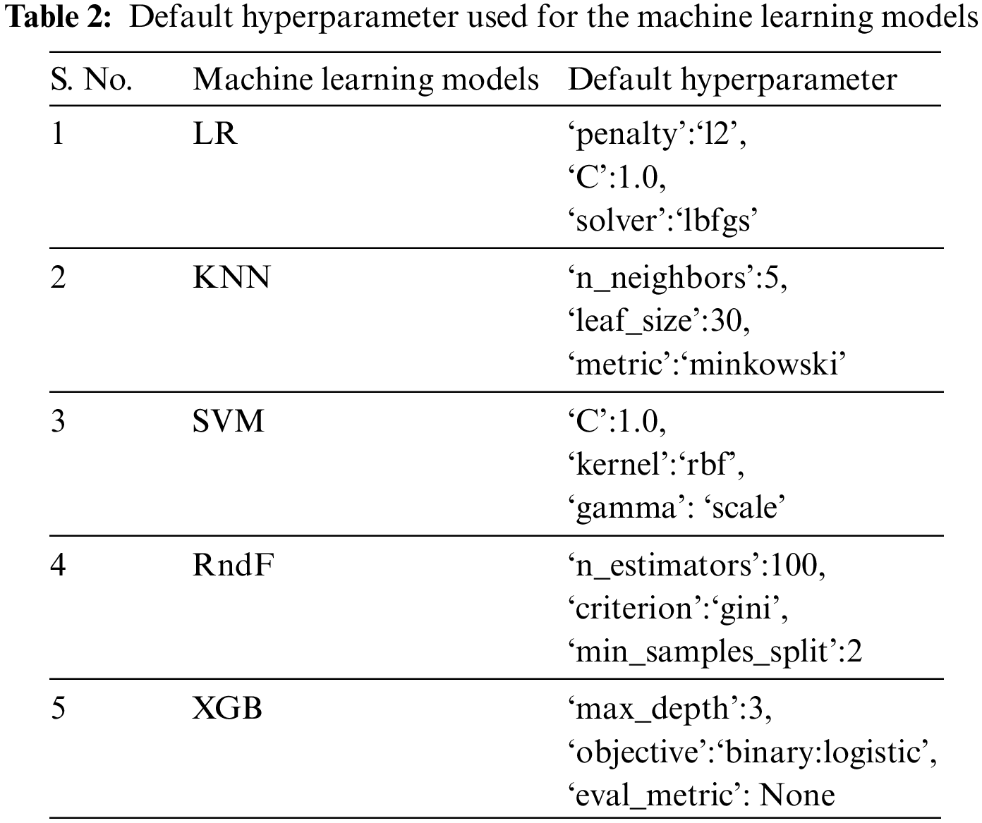
The ML algorithms used on the APD dataset and other benchmark datasets include Logistic Regression (LR), Support Vector Machine (SVM), K-Nearest Neighbor (KNN), Random Forest (RndF), and Extreme Gradient Boosting [36]. Only the default hyperparameter is used for the execution of these ML models, as depicted in Table 2. Different disease datasets have been implemented on these ML models subjected to various HO and CV techniques to investigate if dataset characteristics influence prediction accuracy. The dataset’s essential characteristics are the attribute size, instance size, and categorical and numerical data types.

The dataset is initially split into training and test data sets using the HO method. The training data is used to train ML models, while the test data is used to evaluate the trained model. However, relying on a single HO set makes it challenging to assess the representativeness of the training and test data and the overall stability of the model. To overcome this limitation, the datasets were split into training and testing sets in three different proportions: 4:1 (20% test data), 7:3 (30% test data), and 3:2 (40% test data). However, these splits have their own limitations, such as the potential presence of all positive classes in the training dataset, possible dependencies between the training and test datasets, and uneven distribution of data for training and testing.

Cross-validation is used to overcome these constraints. In CV, the dataset is divided into equal-sized sections called folds. One fold is used as the test set, while the remaining k-1 folds are used as the training set. This ensures that each fold is tested at least once, preventing any overlap in the test data. By adjusting the size of the k fold, it is possible to have similar likelihoods of positive or negative classes. Three alternative folds are commonly used to address this: 3-fold CV, 5-fold CV, and 10-fold CV.

The APD, WBC, CVD, PIMA, CKD, and RA datasets have been collected from multiple sources and are intended for use in the proposed work. Once the data has been collected, its format has been validated to ensure that ML methods may be applied. Consequently, all disease datasets have undergone the required preprocessing stages. The next step follows the fundamental processes of feature engineering, such as addressing missing values using imputation methods and categorical data with one-hot encoding. The preprocessed datasets of diseases are utilized in conjunction with ML classification algorithms and ensemble methods. The final outcome is determined by evaluating the accuracy of the predictions and the CV score produced by the machine learning algorithms.

The accuracy values for different disease datasets, obtained through various HO and CV methods, are presented in Table 3. The suitable ML model detected for the APD dataset is the XGB, with accuracies of 90.48%, 87.1% and 87.8% for different HO methods. In contrast, it obtained 95.1%, 97.1% and 97% accuracy for different CV methods, respectively. Different HO and CV methods evaluated classification accuracy for the remaining datasets, such as CKD, CVD, PIMA, RA, WBC, and APD. These classification accuracies are determined for different datasets to discover whether the dataset characteristics influence the ML model’s performance.

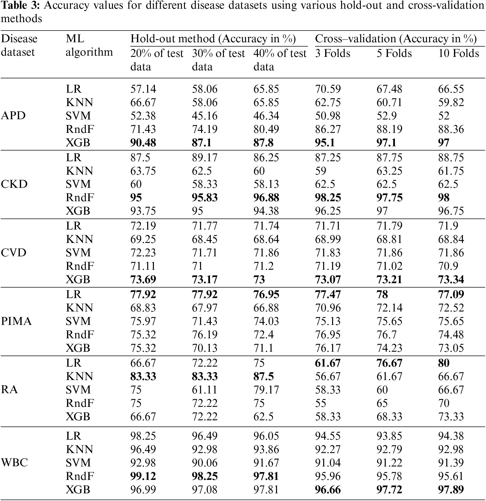
A well-known autoimmune disease is diabetes. The PIMA dataset depicts logistic regression as its efficient ML model because of its linear relationship among the attributes. It consists of 768 instances with eight predictor variables and one outcome variable. LR achieved the highest accuracy compared with other ML models in the PIMA dataset, with accuracy above 75% for all HO methods and CV folds. The K-nearest neighbors (KNN) algorithm performs effectively when applied to datasets that are small in size and have a limited number of features. The RA dataset has 60 data points with eight independent and one dependent variable. The KNN algorithm shows the utmost accuracy above 80% among the various HO methods employed for the RA dataset. At the same time, the accuracy in all CV increases as the number of folds increases in the KNN ML model for the RA dataset.

The WBC dataset has 569 instances with 30 predictor variables and one response variable. RndF achieves the highest accuracy percentage above 97% for all different HO methods. Similarly, XGB shows the highest model performance concerning different CV methods with accuracies of above 96%. The CKD dataset has 400 instances with 24 predictor variables and one response variable. It depicts the highest accuracy, above 95%, in both HO and CV methods. The XGB ensemble technique is the suitable ML model for the CVD dataset with accuracy above 73% for both HO and CV methods, with 70000 samples with 12 independent variables and one dependent variable.

The dataset’s characteristics greatly influence the accuracy score. A prime example is the WBC (breast cancer dataset), which consists of over 500 data points, more than 30 attributes, and no missing values, all of which are continuous numeric attribute values. Consequently, it has been recognized to have the highest accuracy score among other datasets because of its dataset characteristics.

The analysis of the autoimmune arthritis disease dataset identifies the ML model most suited for predicting new patient data, regardless of whether the patient has autoimmune arthritis illness. Similarly, the study discovers biomarkers that are concealed inside the arthritis dataset. In addition, a comparison study of the arthritis dataset and a significant number of benchmark datasets is presented to determine if the dataset’s properties influence the accuracy of the ML model [37]. Arthritis Profile Data identifies ESR, ASO, CRP, RF, L, Abs, Uric Acid, RBC, and TC as significant biomarkers. The researcher has identified significant biomarkers for the autoimmune arthritis data, such as CRP, ESR, and RF [38]. Apart from these important biomarkers, the significant hidden biomarkers discovered are ASO [39], L, Abs, Uric Acid, RBC, and TC. Our empirical evidence demonstrates unambiguously that the XGB ensemble approach provides the best level of accuracy for Arthritis Profile Data.

Among the five ML models, XGB scored the highest accuracy using different HO and CV methods for the APD dataset. It is mandatory to find important features in any dataset [40]. Feature importance values were calculated using the XGB, and the top ten features are displayed in Fig. 5. The first five highest feature importance values are 0.32, 0.27, 0.12, 0.10, and 0.03 for the following features: ESRo, ASO, CRP, RF, and L. ESRo feature holds the highest feature importance value.

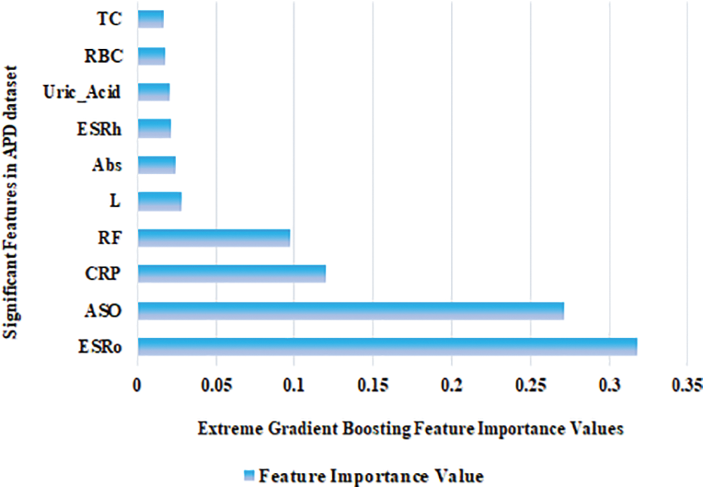
Figure 5: Significant biomarkers identified in the APD dataset

5  Conclusion and Future Scope

Analyzing real-time clinical laboratory data is a crucial task. The APD dataset is the retrospective clinical data collected from the laboratory. The missing data were handled with suitable imputation techniques in the APD dataset. The random and mode value imputer has been identified as the optimal ML imputation algorithms for the APD dataset based on the DoP and residual. The ML algorithm that is most suitable for the APD dataset is XGB. Thus, XGB is an effective ensemble technique for small and high-dimensional datasets. The highest accuracy obtained in the APD dataset is 90.48% for the HO method, which consists of 80% of training data and 20% of test data.Moreover, using five folds CV, it obtained an accuracy of 97.1%. Out of 24 occurrences of the APD dataset, only six significant hidden biomarkers were identified: ASO, L, Abs, Uric_Acid, RBC, and TC. Our empirical investigation demonstrates that dataset properties significantly impact the performance of ML models. Furthermore, the HO method and CV fold size also considerably affect the accuracy of the ML algorithms. Using a larger HO test set or more CV folds generally leads to lower accuracy, as the algorithms can overfit the training data. Finally, as the future scope, we have decided to optimize the accuracy of the XGB using the metaheuristic optimization algorithms.

Acknowledgement: We extend our sincere gratitude to the Editor of the Journal of Intelligent Medicine and Healthcare, for their invaluable guidance. We would like to thank anonymous reviewers whose insights strengthened the quality of the manuscript.

Funding Statement: Department of Science and Technology, New Delhi for the financial support in general and infrastructure facilities sponsored under PURSE 2nd Phase Programme (Order No. SR/PURSE Phase 2/38 (G) dated: 21.02.2017). This work is supported by RUSA Phase 2.0 (II Installment) Grant Sanctioned Vide Letter No. F. 24-51/2014-U, Policy (TN Multi-Gen), Department of Higher Education, Government of India, Dt. 09.10.2018.

Author Contributions: The authors confirm their contribution to the paper as follows: study conception and design, data collection, analysis, and interpretation of results: R. Uma, draft manuscript preparation: S. Santhoshkumar. All authors reviewed the results and approved the final version of the manuscript.

Availability of Data and Materials: Kidney Disease Dataset-https://www.kaggle.com/datasets/mansoordaku/ckdisease. Cardiovascular Disease Dataset-https://www.kaggle.com/code/sakakafayat/cardiovascular-disease-dataset/data. Breast Cancer Dataset-https://www.kaggle.com/datasets/uciml/breast-cancer-wisconsin-data. Diabetes dataset-https://www.kaggle.com/datasets/uciml/pima-indians-diabetes-database. RA Dataset: Data is available on request from the authors. APD Dataset: Data is available on request from the authors.

Conflicts of Interest: The authors declare that they have no conflicts of interest to report regarding the present study.

References

1. L. Runge, “Rheumatology fellowship curriculum,” Ph.D. dissertation, Upstate Medical University, USA, 2001. [Google Scholar]

2. X. Bossuyt, E. de Langhe, M. O. Borghi and P. L. Meroni, “Understanding and interpreting antinuclear antibody tests in systemic rheumatic diseases,” Nature Reviews Rheumatology, vol. 16, no. 12, pp. 715–726, 2020 [Google Scholar] [PubMed]

3. M. A. van Delft and T. W. Huizinga, “An overview of autoantibodies in rheumatoid arthritis,” Journal of Autoimmunity, vol. 110, pp. 102392, 2020 [Google Scholar] [PubMed]

4. Z. X. Xiao, J. S. Miller and S. G. Zheng, “An updated advance of autoantibodies in autoimmune diseases,” Autoimmunity Reviews, vol. 20, no. 2, pp. 102743, 2021 [Google Scholar] [PubMed]

5. “Category: Deaths from autoimmune disease,” Wikipedia: The free encyclopedia. Wikimedia Foundation, Inc., [Online]. Available: https://en.wikipedia.org/wiki/Category:Deaths_from_autoimmune_disease (accessed on 10/12/2022) [Google Scholar]

6. M. G. Chancay, S. N. Guendsechadze and I. Blanco, “Types of pain and their psychosocial impact in women with rheumatoid arthritis,” Women’s Midlife Health, vol. 5, no. 1, pp. 1–9, 2019. [Google Scholar]

7. J. M. Seong, J. Yee and H. S. Gwak, “Dipeptidyl peptidase-4 inhibitors lower the risk of autoimmune disease in patients with type 2 diabetes mellitus: A nationwide population-based cohort study,” British Journal of Clinical Pharmacology, vol. 85, no. 8, pp. 1719–1727, 2019 [Google Scholar] [PubMed]

8. J. Deepack and K. Ishmeet, “Artificial intelligence, machine learning and deep learning: Definitions and differences,” Clinical and Experimental Dermatology, vol. 45, no. 1, pp. 131–132, 2020. [Google Scholar]

9. I. S. Stafford, M. Kellermann, E. Mossotto, R. Mark Beattie, D. Ben et al. “A systematic review of the applications of artificial intelligence and machine learning in autoimmune diseases,” npj Digital Medicine, vol. 3, no. 1, pp. 1–11, 2022. [Google Scholar]

10. R. Uma and S. Santhoshkumar, “Analysis of suitable machine learning imputation techniques for arthritis profile data,” IETE Journal of Research, pp. 1–22, 2022. https://doi.org/10.1080/03772063.2022.2120914 [Google Scholar] [CrossRef]

11. F. Shi, J. Wang, J. Shi, Z. Wu, Q. Wang et al. “Review of artificial intelligence techniques in imaging data acquisition, segmentation, and diagnosis for COVID-19,” IEEE Reviews in Biomedical Engineering, vol. 14, pp. 4–15, 2020. [Google Scholar]

12. R. Zebari, A. Abdulazeez, D. Zeebaree, D. Zebari and J. Saeed, “A comprehensive review of dimensionality reduction techniques for feature selection and feature extraction,” Journal of Applied Science and Technology Trends, vol. 1, no. 2, pp. 56–70, 2020. [Google Scholar]

13. C. Fan, Y. Sun, Y. Zhao, M. Song and J. Wang, “Deep learning-based feature engineering methods for improved building energy prediction,” Applied Energy, vol. 240, pp. 35–45, 2019. [Google Scholar]

14. M. A. H. Abas, N. Ismail, N. A. Ali, S. Tajuddin and N. M. Tahir, “Agarwood oil quality classification using support vector classifier and grid search cross validation hyperparameter tuning,” International Journal of Emerging Trends in Engineering Research, vol. 8, no. 6, pp. 2551–2556, 2020. [Google Scholar]

15. K. Seu, M. S. Kang and H. Lee, “An intelligent missing data imputation techniques: A review,” JOIV: International Journal on Informatics Visualization, vol. 6, no. 1–2, pp. 278–283, 2022. [Google Scholar]

16. J. Poulos and R. Valle, “Missing data imputation for supervised learning,” Applied Artificial Intelligence, vol. 32, no. 2, pp. 186–196, 2018. [Google Scholar]

17. V. Johny, M. Philip and S. Augustine, “Methods to handle incomplete data,” MAMC Journal of Medical Sciences, vol. 6, no. 3, pp. 194, 2020. [Google Scholar]

18. K. Woznica and P. Biecek, “Does imputation matter? Benchmark for predictive models,” arXiv preprint arXiv:2007.02837, 2007. [Google Scholar]

19. A. Sundararajan and A. I. Sarwat, “Evaluation of missing data imputation methods for an enhanced distributed PV generation prediction,” in Proc. of the Future Technologies Conf., Springer International Publishing, pp. 590–609, 2019. [Google Scholar]

20. A. Rasool, C. Bunterngchit, L. Tiejian, M. R. Islam, Q. Qu et al. “Improved machine learning-based predictive models for breast cancer diagnosis,” International Journal of Environmental Research and Public Health, vol. 19, no. 6, pp. 3211, 2022 [Google Scholar] [PubMed]

21. Y. Shinde, A. Kenchappagol and S. Mishra, “Comparative study of machine learning algorithms for breast cancer classification,” Intelligent Cloud Computing Smart Innovation Systems and Technologies, vol. 286, pp. 545–554, 2022. [Google Scholar]

22. Z. Mushtaq, A. Yaqub, S. Sani and A. Khalid, “Effective K-nearest neighbor classifications for Wisconsin breast cancer data sets,” Journal of the Chinese Institute of Engineers, vol. 43, no. 1, pp. 80–92, 2020. [Google Scholar]

23. V. Shorewala, “Early detection of coronary heart disease using ensemble techniques,” Informatics in Medicine Unlocked, vol. 26, pp. 100655, 2021. [Google Scholar]

24. M. N. Uddin and R. K. Haider, “An ensemble method based multilayer dynamic systme to predict cardiovascular disease using machine learning approach,” Informatics in Medicine Unlocked, vol. 24, no. 1, pp. 100584, 2021. [Google Scholar]

25. R. Hagan, C. J. Gillan and F. Mallett, “Comparison of machine learning methods for the classification of cardiovascular disease,” Informatics in Medicine Unlocked, vol. 24, pp. 100606, 2021. [Google Scholar]

26. N. A. Baghdadi, S. M. Farghaly Abdelaliem, A. Malki, I. Gad, A. Ewis et al. “Advanced machine learning techniques for cardiovascular disease early detection and diagnosis,” Journal of Big Data, vol. 10, no. 1, pp. 1–29, 2023. [Google Scholar]

27. U. Banu and K. Vanjerkhede, “Hybrid feature extraction and infinite feature selection based diagnosis for cardiovascular disease related to smoking habit,” International Journal on Advanced Science, Engineering & Information Technology, vol. 13, no. 2, pp. 578–584, 2023. [Google Scholar]

28. B. P. Kumar, “Diabetes predictiion and comparative analysis using machine learning algorithms,” International Research Journal of Modernization in Engineering Technology and Science, vol. 4, no. 5, pp. 4688–4696, 2022. [Google Scholar]

29. V. Chang, J. Bailey, Q. A. Xu and Z. Sun, “Pima Indians diabetes mellitus classification based on machine learning (ML) algorithms,” Neural Computing Applications, vol. 35, no. 22, pp. 16157–16173, 2022. [Google Scholar]

30. D. Elias and T. Maria, “Data-driven machine-learning methods for diabetes risk prediction,” Sensors, vol. 22, no. 14, pp. 5304, 2022. [Google Scholar]

31. E. M. Senan, M. H. AI-Adhaileh, F. W. Alsaade, T. H. Aidhyani, A. A. Alqarni et al. “Diagnosis of disease using effective classification algorithms and recursive feature elimination techniques,” Journal of Healthcare Engineering, vol. 2021, pp. 1004767, 2021 [Google Scholar] [PubMed]

32. V. Chaurasia, M. Pandey and S. Pal, “Chronic kidney disease: A prediction and comparison of ensemble and basic classifiers performance,” Human-Intelligent Systems Integration, vol. 4, no. 1–2, pp. 1–10, 2022. [Google Scholar]

33. S. Tekale, P. Shingavi, S. Wandhekar and A. Chatorikar, “Prediction of chronic kidney disease using machine learning algorithm,” International Journal of Advanced Research in Computer and Communication Engineering, vol. 7, no. 10, pp. 92–96, 2018. [Google Scholar]

34. M. Majid, Y. Gulzar, S. Ayoub and F. Khan, “Using ensemble learning and advanced data mining techniques to improve the diagnosis of chronic kidney disease,” International Journal of Advanced Computer Science and Applications, vol. 14, no. 10, pp. 470–480, 2023. [Google Scholar]

35. U. Ramasamy and S. Sundar, “An illustration of rheumatoid arthritis disease using decision tree algorithm,” Informatica, vol. 46, no. 1, pp. 109–119, 2022. [Google Scholar]

36. H. Zhou, Y. Xin and S. Li, “A diabetes prediction model based on Boruta feature selection and ensemble learning,” BMC Bioinformatics, vol. 24, no. 1, pp. 1–34, 2023. [Google Scholar]

37. M. Al-Tawil, B. A. Mahafzah, A. Al Tawil and I. Aljarah, “Bio-inspired machine learning approach to type 2 diabetes detection,” Symmetry, vol. 15, no. 3, pp. 1–16, 2023. [Google Scholar]

38. D. Aletaha, T. Neogi, A. J. Silman, J. Funovits, D. T. Felson et al. “2010 Rheumatoid arthritis classification criteria: An American College of Rheumatology/European League Against Rheumatism collaborative initiative,” Arthritis & Rheumatism, vol. 62, no. 9, pp. 2569–2581, 2010. [Google Scholar]

39. R. J. François, “Beta-haemolytic streptococci and antistreptolysin-O titres in patients with rheumatoid arthritis and a matched control group,” Annals of the Rheumatic Diseases, vol. 24, no. 4, pp. 369, 1965. [Google Scholar]

40. R. Asa, L. Busi and J. S. Meka, “A hybrid deep learning technique for feature selection and classification of chronic kidney disease,” International Journal of Intelligent Engineering & Systems, vol. 16, no. 6, pp. 638–648, 2023. [Google Scholar]