Contributions of Remote Sensing and GIS to the Inventory and Mapping of Colonial Geodetic Markers in the Katangese Copper Belt

1  Introduction

The geodetic markers of a country are a framework of triangulation points of known coordinates which serve as a basis for topographic work. They are of obvious scientific interest such as: computing of new point coordinates, definition of the exact shape of the terrain, economics, production of the base map, and derived maps and plans. They are therefore essential supports for the management of the quantity and quality of geometric or trigonometric triangulation networks.

Recent studies on the impact of human activities on forest ecosystems and mining in the Katanga’s Copper Belt (KCB) reveal significant environmental disturbances, particularly due to deforestation and unregulated mining practices [1,2]. Soyer et al. [3] noted a rapid increase in open clearings in the Lubumbashi’s forest from 230 km² in 1973 to 1,630 km² in 1981. Malaisse et al. [4] found that natural forest formations are now limited to a 25–30 km radius around the city. Furthermore, Bizangi [5] highlighted carbonization practices causing a deforestation rate of 40,000 hectares annually in Shaba. Following the same trends, Cabala Kaleba et al. [2] reported a decrease in the forest recession front from 49% to 42% between 2002 and 2015, emphasizing the urgent need for sustainable practices to address environmental challenges in the region.

Mining has gone through three main stages [6]: (1) the creation of the Union Minière du Haut Katanga (UMHK), which became Générale des Carrières et des Mines (GCM), and of the Société de Développement Industriel et Minier du Congo (SODIMICO), which became SODIMIZA when the Congo was called Zaire and was bought by GCM in 1987, (2) the creation of the Société Minière de Tenke Fungurume (SMTF), the precursor of the current Tenke Fungurume Mining TFM which ended its operations in 1977–78 and (3) finally, the creation of TFM was established in 1996. These companies operated in very distinct, restricted and controlled areas. This third stage, coincides with the liberalization of the mining sector, initiated in 1997 by President Laurent Désiré Kabila. The effect of this was, and still is, a craze for anarchic mining by national and foreign researchers of cobalt-rich heterogenite or copper-rich malachite. In line with this anarchy, in 2009, the Mining Registry and the Division of Mines granted 4,263 quarries and mining titles to mining companies, of which 1,663 (39%) were granted to the province of Katanga alone. In addition, more than 45 companies received 23,450.13 km² for artisanal exploitation.

In addition to the regression of forests, of which the disfigurement of landscapes and the degradation of soils are some of the inevitable consequences, the proliferation of mineral extraction sites is also accompanied by abrupt alterations of the relief, in particular the razing of mineralized hills and the creation of cuttings, embankments and new mounds, as can be observed at the Luiswishi sites [6]. Furthermore, whereas during the period 1906 to 1996, the materialized geodetic network by fixed and resistant markers was maintained intact, since the liberalization of mining [7,8], these markers, considered as indications or clues of mineralization, have become targets of destruction. However, hills are privileged sites for the establishment of geodetic markers which must be placed in such a way as to be visible from one another.

The scarcity of accurate synoptic topographic data in the region, both current and historical, available to the public is prompting the development of new analytical approaches to monitor geomorphological mutation and the completeness of geodetic benchmarks in the KCB. Under these conditions, remote sensing techniques, notably satellite RADAR, become essential for characterizing the past and present state of landforms. Satellite RADAR offers the possibility of characterizing topographic variables and adjacent phenomena such as: Soil erosion [9,10], Geophysical measurement [11], and Vertical Land Change due to surface mining [12]. RADAR-derived data such as SRTM1, ASTER GDEM2, ALOS3, and TanDEM-X4, can be used on the one hand, to characterize and monitor topographic changes [13,14]. On the other hand, it can help to assess the accuracy of Digital Terrain Models (DTMs) compared with other data sources for inventorying and observing landform change through geomorphological and statistical approaches [15–17].

In this study, we aimed to analyze the potential applicability of SRTM data for the monitoring of macroscopic terrain mutations and the indirect inventory of geodetic markers. Since there is a paucity of similar work, our research had drawn on work by [15,16,18]. These authors spread out the approaches to accuracy assessment and exploitation of SRTM data, but do not significantly integrate the aspect of inventory of geodetic landmarks and the characterization of their geomorphological changes. However, Gaye [19] proposed the use of GIS in the context of triangulated network management. An overview on the application of mathematical and statistical methods in the analysis of topographic data can be found in the publications of [20–22].

This study, which covers an area of 42,980 km², representing 8.75% of the Katanga Province, uses Geographic Information Systems (GIS), remote sensing, statistics and spatial analysis to carry out a remote inventory of the geodetic markers installed by the Belgians in the beginning of the 20th century. First, we made a statistical analysis to assess the complementarity of the Comité Spéciale du Katanga (CSK) historical topographic data, SRTM and UAV data for geomorphological characterization. On the other hand, we explore spatial autocorrelation analysis to assess and validate change on a geodetic landmark using these data. Apart from the introduction and conclusion, the second section of this work presents our study area and our material and methods. We then present the obtained results in Section 3, and in Section 4, we discuss these results and present some perspectives.

2  Material and Method

2.1 Study Area

The coordinates of 25° and 27° East, and −10° and −12° South, fix the study area at approximately 42,980 km2, between the Haut Katanga and Lualaba provinces. Negligible encroachment into Haut-Lomami and Tanganika provinces is observed. The area extends north-west and south-west beyond the boundaries of the KCB, where mining and related activities are concentrated (see Fig. 1).

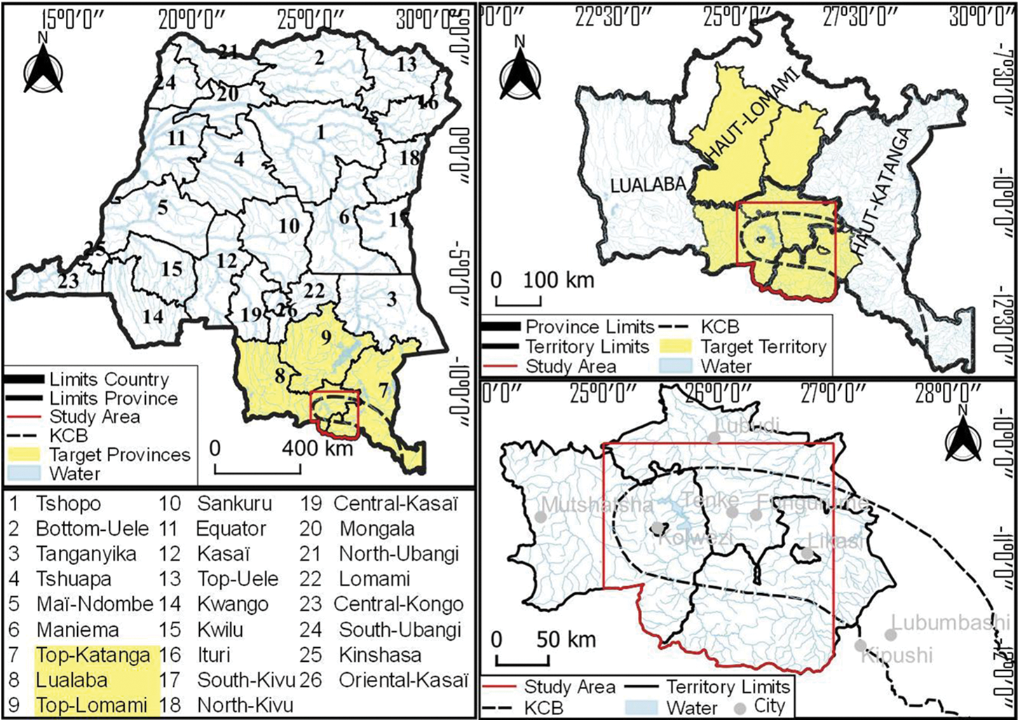
Figure 1: Location of the study area including the KCB

The Katangese Copper Belt runs from Namibia to the Congolese stalk via Solwezi in Zambia. This curvature, was naturally accompanied by various accidents: faults, thrusting and various breaches that favored the uncovering of older stratiform mineralization and created a second mineralizing occurrence in the major faults. With a geostrategic connotation, the KCB contains, according to Dikumbwa et al. [23], copper and cobalt mining zones in Zambia and the DRC that are arranged on folded sediments. Furthermore, Lerat [24] reported that copper in Katanga seems to have been known or at least suspected long before the colonial occupation (1798). Details on the geological environment and the support of the mineralization in the KCB are recorded in the publications of [25–28], combining petrology, stratigraphy, geomorphology, tectonics and metallogeny in order to characterize the geology of the Katanga’s deposit. Kampunzu et al. [29] determined the extent and ages of the sedimentary strata containing the copper and cobalt ores.

According to Lerat [24], the industrial development of Katanga’s mineral deposits dates back to colonial times. Maury [30] stated that before and during the development of the copper-bearing basin in southern Katanga, several explorations [25] and missions (Anglo-Belgian (1911 and 1913); Belgian-Portuguese (1915 and 1920)) and geodetic, topographic and cartographic missions were carried out respectively to materialize the Katango-Rhodesian and Katango-Angolan borders and to construct the triangulations network of first, second and third order [31] (CSK 1936), which served to support the colonial economic development plan [32]. Although it is less developed nowadays by the Institut Géographique du Congo (IGC), this network provides the best planimetric and altimetric references locally. It is currently poorly documented in the field but remains well documented.

In the study area, the setting of geodetic markers was based on relative methods and included more than 442 triangulation points, of which at least 64 were of the first order, supplemented by about 226 second-order markers and about 144 third-order markers. The categories of the other 8 geodesic markers have not been identified on the map. The procedures for their placement were well defined. The margins of error for the Katanga network were: ±0”,52 (in X), ±0”,42 (in Y) and ±0”,64 (in Z) for the trigonometric levelling of a 10-kilometer range. The resulting cartographic exploitation of the data is adapted to the fundamental two-parallel Lambert conic projection, which is considered robust for cadastral exploitation. The Gaussian conformal system presents important deformations limiting its use [30]. It simply expresses its unsuitability to the physical conditions of the natural environment with its uneven topography; consequence of endogenous geological phenomena, responsible for the outcropping of copper and cobalt mineral deposits on certain hills in the KCB.

2.2 Methodology

2.2.1 Data

Three data sources were used: (1) 4 topographic maps numbered S11/25, S12/25, S11/26 and S12/26 representing the 1st, 2nd and 3rd order triangulation network, based on surveys carried out between 1922 and 1929 by the CSK, (2) 22713 elevation points from a high-precision (1 m) topographic survey carried out with a Phantom 4 RTK UAV on 22/11/2021, in a small portion of 2 km² to the west of our study area indicate in Fig. 2 and (3) the SRTM data of an arc-second of 2000, downloaded via the Earth Explorer platform covering our study area.

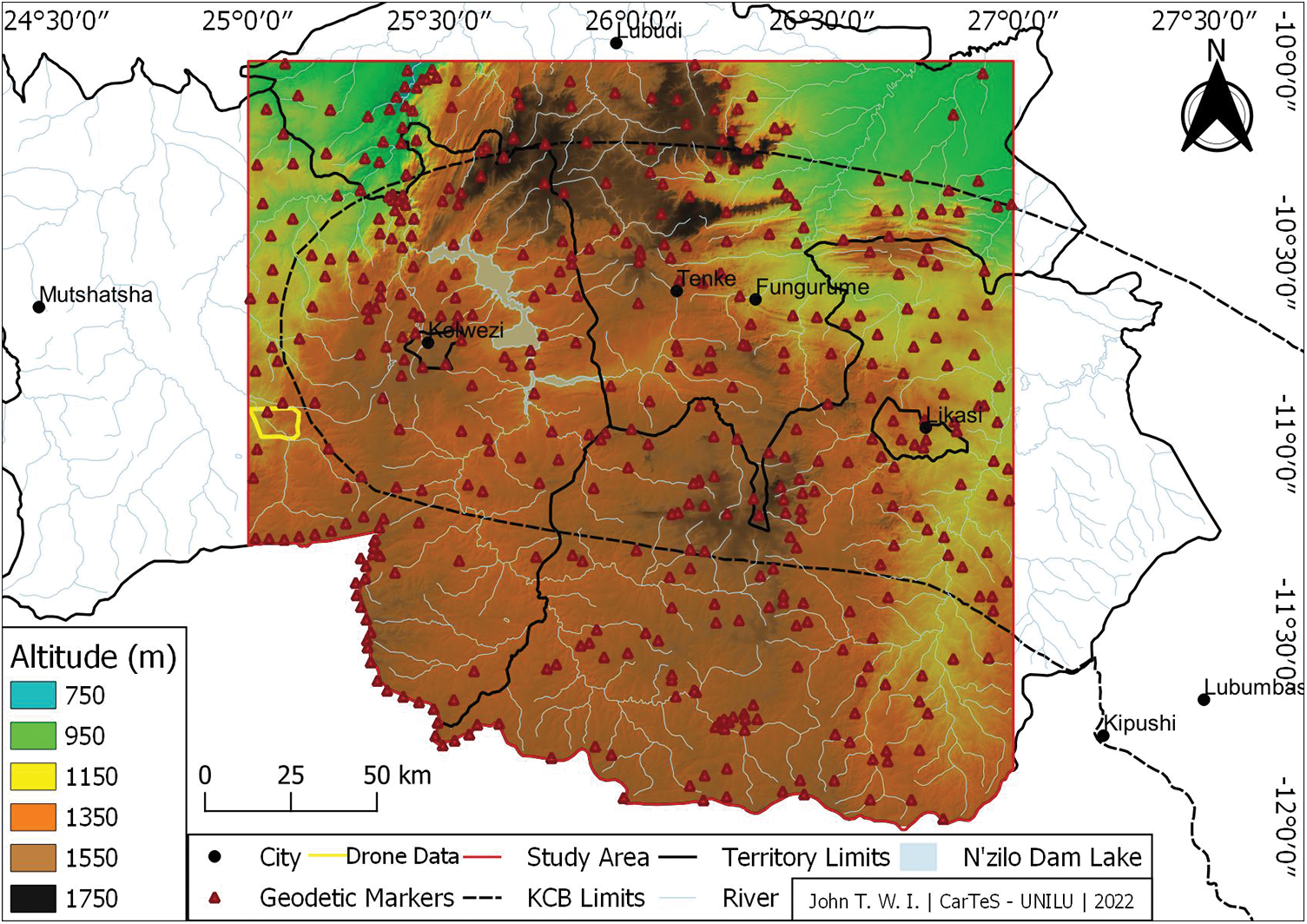
Figure 2: Planimetric and altimetric sampling points on the SRTM image

The Katanga triangulation network is based on 9 bases measured between 1912 and 1951. According to Straeten [8], the definitive calculation was based on fundamental chains divided into closed circuits, adjoining each other. These circuits were rigorously compensated by the method of conditional equations subject to the law of least squares, in order to achieve exact closures on the geodesic bases and on the fixed elements of the connection to the circuits already compensated [33]. The entire network thus formed a rigid framework in which all closure errors were eliminated.

Firstly, the topographic maps were used to extract the 442 points representing the elevation levels of the CSK geodetic markers. In a second step, a raster of 30 m spatial resolution was obtained by interpolating the 442 CSK points. We then reprojected the 22713 points cloud collected from the UAV and the SRTM in UTM zone 35S for further processing. This process admitted errors of around 0.73 m in X and Y for the SRTM and around 0.026 m in X and Y for the point cloud, compared with the CSK maps; admissible for pixel resolutions of 30 m (SRTM) and 1 m (UAV), respectively [34].

Three paired samples of points were then formed. The first corresponds to the elevations in 1922 and 2000 using the original 442 CSK points in 1922 and the extraction of values from the SRTM of 2000 on the same points location. The second corresponds to the elevations in 1922 and 2021 using the 22713 UAV to extract the values on the CSK raster of 1922 and the original UAV values. Finally, the third corresponds to the elevation in 2000 and 2021, using the 22713 UAV to extract the values on the SRTM and the original UAV values. The last two matched samples represent the area covered by the UAV.

2.2.2 Method

The methodology used for this study is based on the variance analysis, in the spirit of Derrick et al. [35] in order to compare the different paired data and the analysis of spatial autocorrelation and shrinkage estimators to characterize the change. The change in elevation on a landmark by considering the set of changing landmarks, in reference to [36,37], is outlined below.

2.2.3 Statistical Analysis

The descriptive evaluation of the data series based on normality tests allowed to measure the altimetric distributions of the CSK and SRTM bounds of orders 1, 2 and 3, via the skewness and Kurtosis coefficients:

α3=n∗±M3(n−1)∗(n−2)∗σ3(1)

α4=n(n+1) ∗ M4−3∗M22∗(n−1)(n−1)∗(n−2)∗(n−1)∗σ4(2)

With α3 the skewness coefficient, α4 the Kurtosis coefficient, n: the number of observations, σ the standard deviation, Mn (the moment n) = ∑(xi−X¯x)n.

For this purpose, we will note the symmetry when Skewness α3 = 0. If α3 > 0, we consider a positive skewness. If α3 < 0, there is a spread of elevations to the left of the distribution curve.

The multiple regression of the CSK, SRTM and UAV datasets aimed to reduce the influence of the divergence of the measurement systems used for the surveys and improve the comparative analysis. This made it possible to correct the errors in the SRTM and UAV elevation measurements from the CSK topographic data set. With the CSK geodetic markers as explanatory variables and the SRTM and UAV elevation observations as dependent variables. The residual values provided by the regression model constituted the theoretical deviations to be subtracted.

We calculated the linear regression coefficients: α1′, α2′ and α3′ by solving a system of p−1 equations with p−1 unknowns for the set from equations: r1p = a1+′r12a2′ + r13a3′; r2p = a2+′r21a1′ + r23a3′; r3p = a3+′r31a1′ + r32a3′. To do this, we proceeded by successive substitutions: a1′= r1p−r12a2′+r13a3′. Hence, r2p = a2+′r21(r1p−r12a2′ + r13a3′)+r23a3′; a2′=r2p−r21a1′+r23a3′ and a3′=r3p−r31a2′+r32a3′. p is the variable, p−1 the independent variable and r12,r13,…,rpp the linear correlation coefficients of the pairs of variables with: s1,s2,…,sp, their standard deviations, after calculating the multiple regression coefficients of the CSK, SRTM and UAV series by: α1=α1′SySx1;α2=α2′SySx2;α3=α3′SySx3.

The quality control of the multiple regression was based on the fit constant resulting from the solution of the equation coordinated at the origin : ∈ = y−α1x1−α2x2−α3x3, and the coefficient of determination R2=∑j−1p−1αj′rjp, that influence the multiple correlation coefficient LAFFLY (2006):

(ryx12+ryx22)−2(ryx1.ryx2.rx1x1)1−rx1x22=Ryy(3)

The equal sample sizes allowed the study to analyze the homogeneity of the variances of the CSK and SRTM series. Using the Levene [38] and Brown et al. [39] tests, which are considered robust for the 56 supposed tests. The LEVENE algorithm is noted:

L=(N−k)∑i=1kNiX¯ij−X¯(k−1)∑j=1k(X¯ij−X¯)2(4)

With Vij=|Xij−X¯i|,i=1,…,k;j=1,…,n and X¯i the median of the elevation data series. The FORSYTHE (F) test of equality of variances is based on ANOVA from transformations of the response variable. In its application we measured the spread of groups by the formula: Zij=|Yij−Y¯i|, before calculating F which is equal to:

N−pp−1∗∑ip=1nj(z¯j−z¯)∑ip=1∑j=1nj(z−Z¯¯j)2(5)

The F-test is done with degrees of freedom written as: d1=p−1 and d2=N−p. The confidence interval of two-sided standard deviation of similar orders of the two series CSK and SRTM was found with the Bonferroni method using the confidence level: 1−α2p. Where, Y¯ is the median of groups j,p,nj and N are respectively the numbers of group, of observations in the group and the total of observations. Z¯j are the group means of Z¯ij and Z¯ is the overall mean of zij.

2.2.4 Mathematical Expression of Elevation Change on a Geodetic Datum

The preceding statistical parameters led to the formulation of a first mathematical expression for the variation of a controlled elevation z from the point P(xy) at times T1(z) and T2(z′) which is written:

VzP=zP−z′P≠−σ−1.5m and σ+1.5m(6)

With VzP the variation in elevation in meter at the observation point P(xy),zP the elevation measured at point P at time T1 (elevation measured by the CSK)\!, z′P the elevation measured at the same point P(xy) at time T2 (provided by the SRTM).

If VzP is negative: VzP<−σ−1.5m the part is buried and if VzP>−σ−1.5m the part is exhumed. If VzP=−σ−1.5m or VzP=σ+1.5m=>zP=z′P. The above argument had shown limitations filled by the analysis of the intensity level of the bilateral spatial association of the locations of the changing landmarks.

2.2.5 Mathematical Expression of Elevation Change on a Geodetic Datum

Spatial exploratory analysis of CSK and SRTM data has identified the locations of atypical and extreme elevation variations at selected geodetic markers. By identifying their spatial clustering patterns and associations, punctuated by various forms of spatial heterogeneity.

From the spatial autocorrelation of elevation changes on 442 geodetic markers we measured the intensity of the variation of an elevation zi observed at time ti−1 from the current value (zj) raised at time t and the level of the bilateral association of the latter with its neighbors ωij. If the similarity between the changing neighboring markers controlled from zi, an element of the matrix ω, decreases with distance, the spatial autocorrelation is considered positive. It is negative if nearby landmarks tend to have more different elevation changes than more distant landmarks and finally it is null when no relationship exists between the proximity of the variations on the geodesy points and their degree of similarity. Thus, the study was able to identify and exclude locations that showed aberrant elevation changes.

Modelling such spatial interactions requires specifying the spatial links between each geodetic marker. All these links were recorded in a square spatial connectivity matrix (W). Having rows and columns equal to the number of terminals (ω) and where each term zi represents how point i and its neighbour j are spatially connected. Thus, the spatial connectivity matrix exogenously specified the topology of the spatial system and the choice of these links was made according to the needs of the analysis. In this study, we used in turn a matrix of 442 and 79 geodesic terminals.

The validation of elevation variations on markers is based on Moran’s bivariate scatterplots (IB) and change removal estimator algorithms. The methods for constructing the IB and its variants are proposed by [40–45]. The study found that the theoretical IB is equal to:

∑i(∑j(ωijyi)∗xi)∑ixi2(7)

where ωy is the slope of a spatial regression on xintegrating measurements at two points in time: zi,t and Zj,t−1. The reliability of the change in elevation then relates to the extent to which the value observed at one location at one time is correlated with other variations at neighbouring locations at the different time. It is written: zi,t to ∑jωijzj,t−1, i.e., so the correlation between a change at time t and its neighbours at time t−1 is equal to:

∑i(∑j(ωijyi,t−1)∗xi,t)∑ixi,t2(8)

∑i(∑j(ωijyi,t−1)∗xi,t−1)∑iZi,t−12(9)

The integration of this dynamism will be written: zi,t=β1∑jωijzi,t−1+μi. Considering ωij as an error term, the previous formula becomes: zi,t−1=β2∑jωijzi,t−1+μi.

β1 indicates the dynamic process, β2 measures the degree of spatial correlation between past and current central elevations. Then, the relevance of a change on a boundary will be interpreted from the bivariate spatial association integrating β3, following the relation: ∑jωijZi,t−1=β3zi,j+μi.

The results of the IB reveal the degrees of spatial associations of the elevation variations with pseudo-values (p 0.05, p 0.01 and p 0.001), the orientation and slope of the regression line, the dispersion of the points in the quadrants: high-high, high-low, low-low and low-high of the Moran diagram.

The choice of the methodology used in this research is privileged by the contexts: lack of inspections of geodetic markers, data updates, physical inventories and maintenance of the triangulation network, throughout the national territory by the commissioned body.

3  Results

3.1 Distributions and Spatial Correlations of CSK and SRTM Topographic Data

3.1.1 Group (Order) Distributions of the CSK and SRTM Data Sets

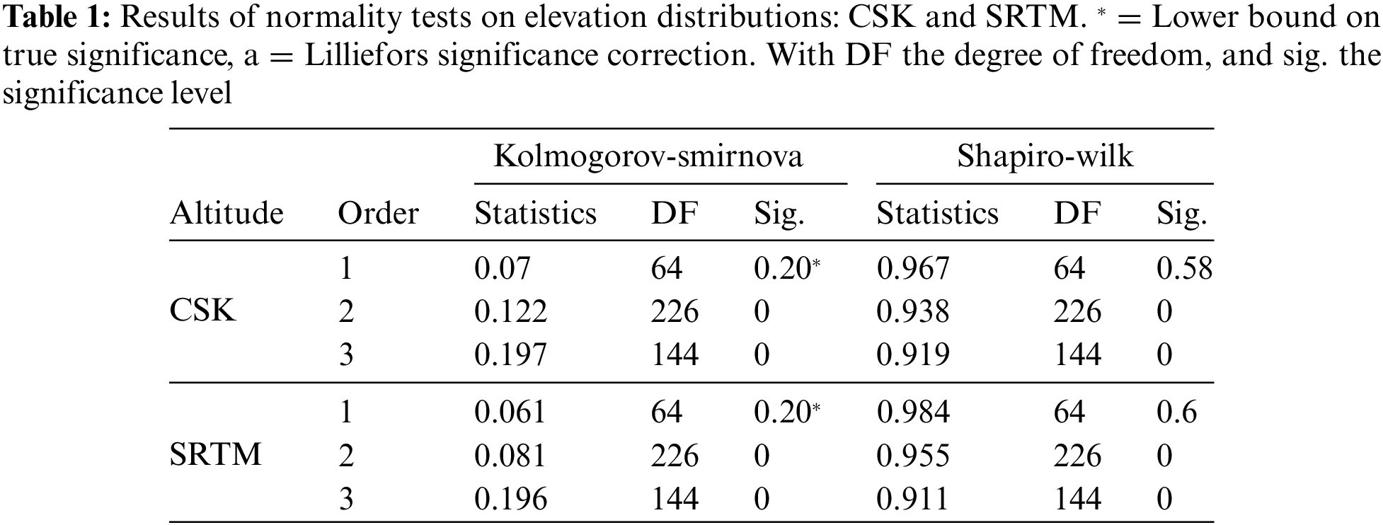
The altimetry data under study show a majority of asymmetrical patterns spread out to the left (Figs. 3A and 3C). The elevation variables follow a random distribution. Skewness coefficients are respectively: −0.94 and −0.79; −0.85 and −0.84, for orders: 2 and 3 of the two observation series CSK and STRM. The box plots (Figs. 3B and 3D) for the first-order CSK and STRM geodesic markers show normal distributions, in contrast to those for orders: 2 and 3. Fig. 3E shows the regression models for the two paired data series. Results in Figs. 3A and 3C are confirmed by the Kolmogorov-Smirnov normality tests, shown in Table 1 below.

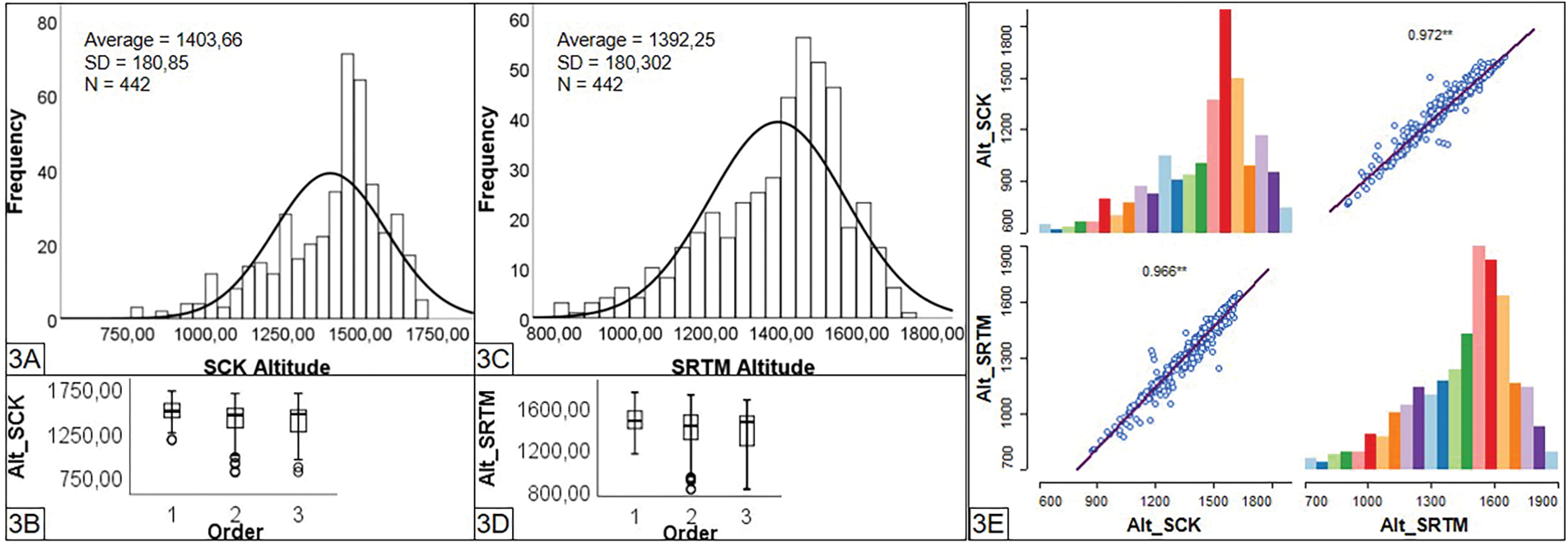
Figure 3: Distributions and correlations of CSK (1952) and SRTM (2000) elevations observed on 420 geodetic markers

Unlike all statistical tests, the normality test seeks to accept H0. The alpha (Sig) significance levels of zero in the results of the main normality tests prove that groups 2 and 3 of the CSK and SRTM data sets follow asymmetric distributions for both Kolmogorov (non-parametric and flexible) and Shapiro-Wilk (parametric and specific) tests. The two groups (2 and 3) were subsequently analyzed differently from the CSK and SRTM of order 1 which did not undergo any transformation to stabilize the group variances.

3.1.2 Group (Order) Distributions of the CSK and SRTM Data Sets

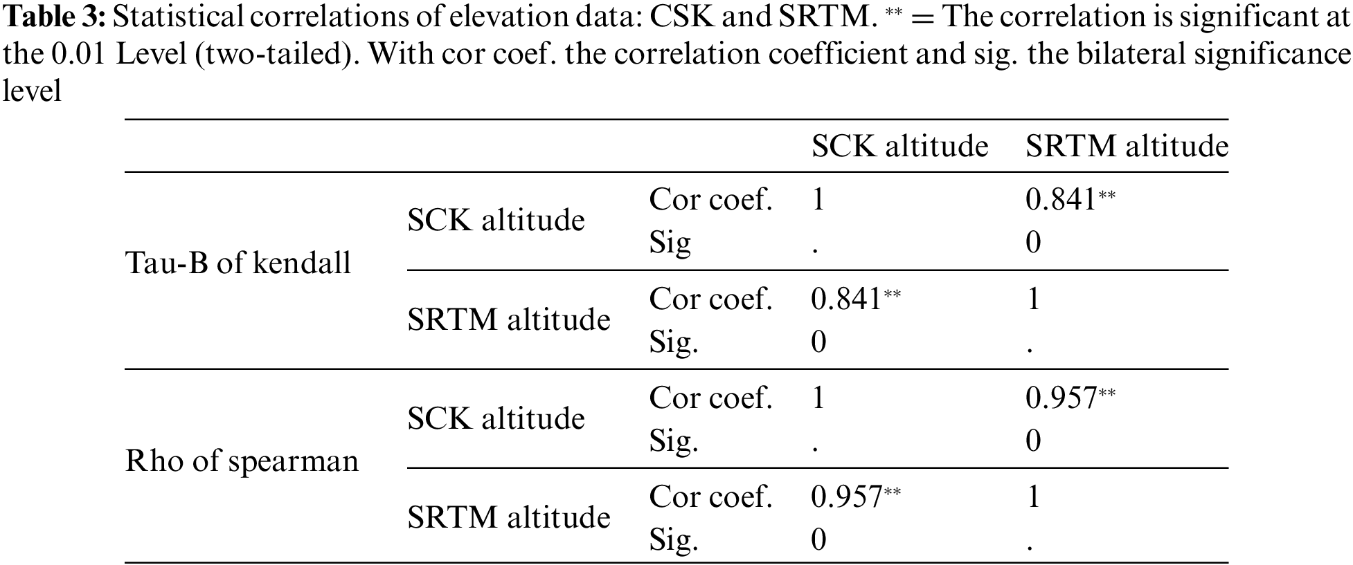
The two-way spatial correlations of the two elevation series (Fig. 3E) show a strong relationship: 0.966 SRTM-CSK and 0.972 CSK-SRTM. Statistical tests applied to the two linked data samples (CSK and SRTM) show a good level of significance of their relationship, as shown in Tables 2 and 3. Spearman’s Rho provides the best score (0.957) in contrast to the result (0.841) obtained with Kendall’s algorithm.

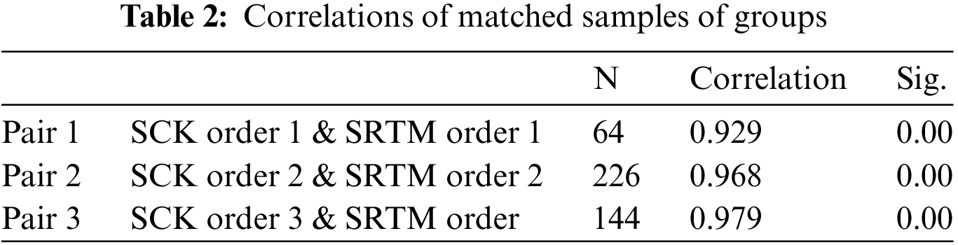
One would expect very good relationships between CSK and SRTM individuals in the same groups. Pairs of orders 1 and 3 form the extreme correlation bounds of 0.929 and 0.979, respectively.

3.2 Statistical Difference of CSK and SRTM Topographic Data Groups

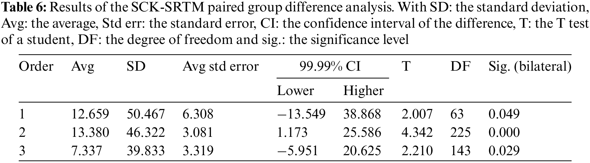
The comparative study of individuals from the CSK and SRTM topographic data groups shows differences in the statistical means of the elevations of the markers, respectively: 1 (1483.2063 m for and 1470.5469 m); 2 (1395.7690 and 1382.3894 m) and 3 (1380.1286 and 1372.7917 m) (see Figs. 4A–4H). The differences of averages of geodetic markers between the CSK and SRTM is about: 12.6594 m for order 1, 13.3796 m for order 2 and 7.3369 m for order 3.

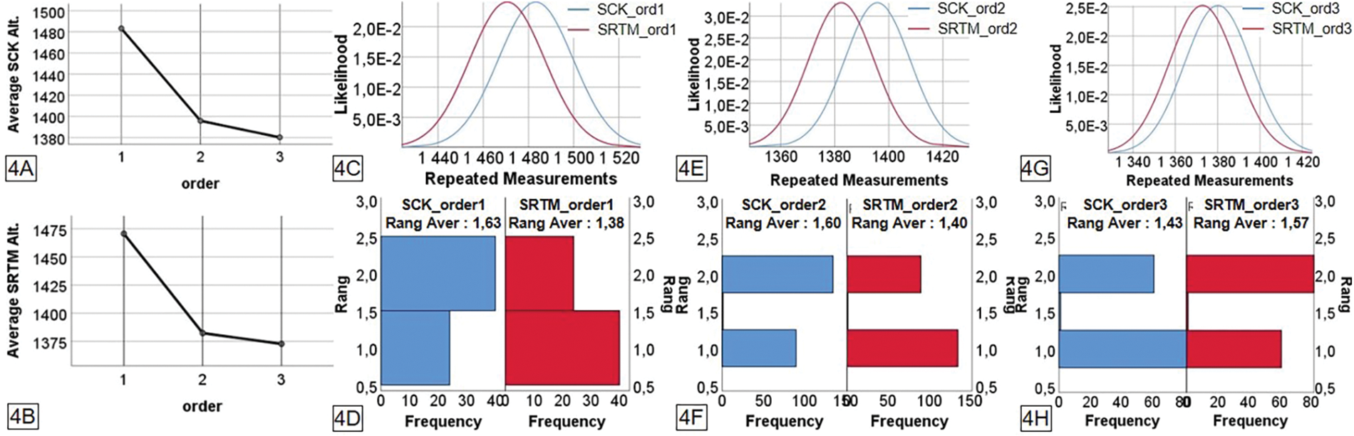
Figure 4: A and B are the mean elevations of orders 1, 2 and 3 of the CSK and SRTM data series. C, E and G: The posteriori distributions of the series averages with repeated measurements for the same orders considered. D, F and H: The two-factor variances by Friedman ranking for matched altimeter samples of the said orders 1, 2 and 3

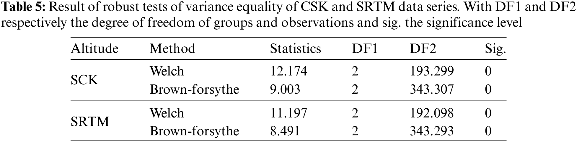
The results of the likelihood analyses (Figs. 4C–4E) show that the CSK elevation series of orders: 1, 2 and 3 are different from the SRTM series of the same orders. The robust tests (Table 4) prove this. The study of variances was carried out a priori on the distribution of matched averages, in order to find, according to Bayes’ central limit theorem, at a 99.99% credibility interval, the degrees of difference expressed by the data under examination. The coefficients: 0.063; 0.04 and 0.021, of Kendall’s agreement (W) obtained respectively at 1 dl for the two-factor analysis of variance and Friedman’s classification for matched samples (Figs. 4D, 4F and 4H) confirm this difference. The differences of: 0.25; 0.20 and −0.14, are observed respectively at the mean ranks between the CSK and SRTM geodetic markers of orders: 1, 2 and 3. This shows the topographic change, to be characterized spatially from the 442 observation points that the study exploits.

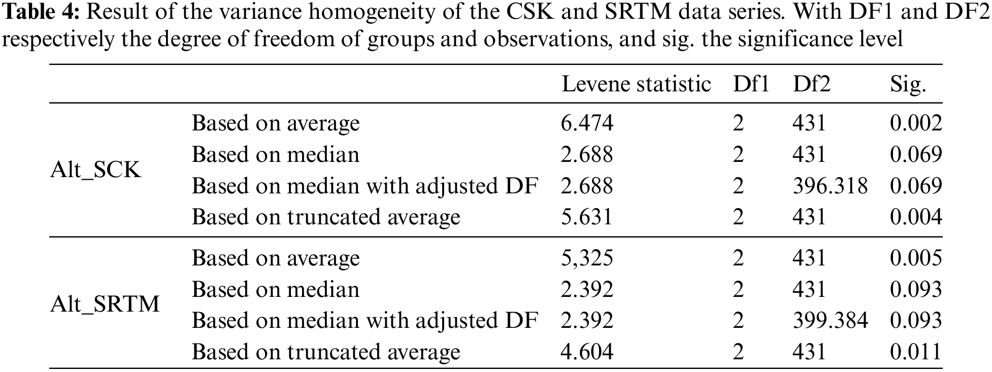
The analysis of equal variances (Tables 4 and 5) carried out with both the Levene statistic and the Welch and Brown robust tests shows that the CSK and SRTM series do not have the same altimeter variances. The hypothesis of homogeneity of variances must be rejected.

3.3 Assessment of Changes Based on Matched Differences in CSK and SRTM Elevations of Orders: 1, 2 and 3

These analyses allowed the study to take into account errors in the assessment of elevation changes. This is due both to the differences in the techniques used during the collection of CSK and SRTM data and to the different levels of accuracy offered by the instruments used in the determination of elevations by the operators. Depending on the order of the geodetic datum, the tolerance ranges of the variation of an elevation are fixed by the confidence intervals of the difference shown in Table 6. In order to further eliminate such errors of assessment, the research considered the standard deviations of the differences to evaluate the altimeter changes on the 442 CSK and SRTM observation points. Thus, three indexing queries support this approach. For the pair of order 1 geodetic markers it is written: zP−z′P≤−50.467−1.5 or zP−z′P≥50.467+1.5; for the pair of order 2 zP−z′P≤−46.322−1.5 or zP−z′P≤46.322+1.5, and for the pair of order 3 zP−z′P≤−39.833−1.5 or zP−z′P≤39.833+1.5. These values are all in meter (m).

3.4 Distributions and Spatial Relationships of Elevation Differences in the CSK-SRTM, CSK-UAV and SRTM-UAV Data Sets

The analysis integrating more than 22,000 points surveyed in 2021 with a UAV, on a small control area, allows the arbitration of the observed elevation differences between the CSK and SRTM data sets (Fig. 5). The differences between the SRTM and UAV elevations are very small, as shown in graph A3, having a normal distribution with no bilateral SRTM-UAV and UAV-SRTM correlations, despite the consideration of the spatial dimension of the observation points. The CSK-SRTM and CSK-UAV elevation differences follow an asymmetric distribution. Visible through graphs B1 and B2 and histograms A1 and A2, supported by better alignments of observations on the respective regression lines. This encourages the use of SRTM data, evaluated by the present study.

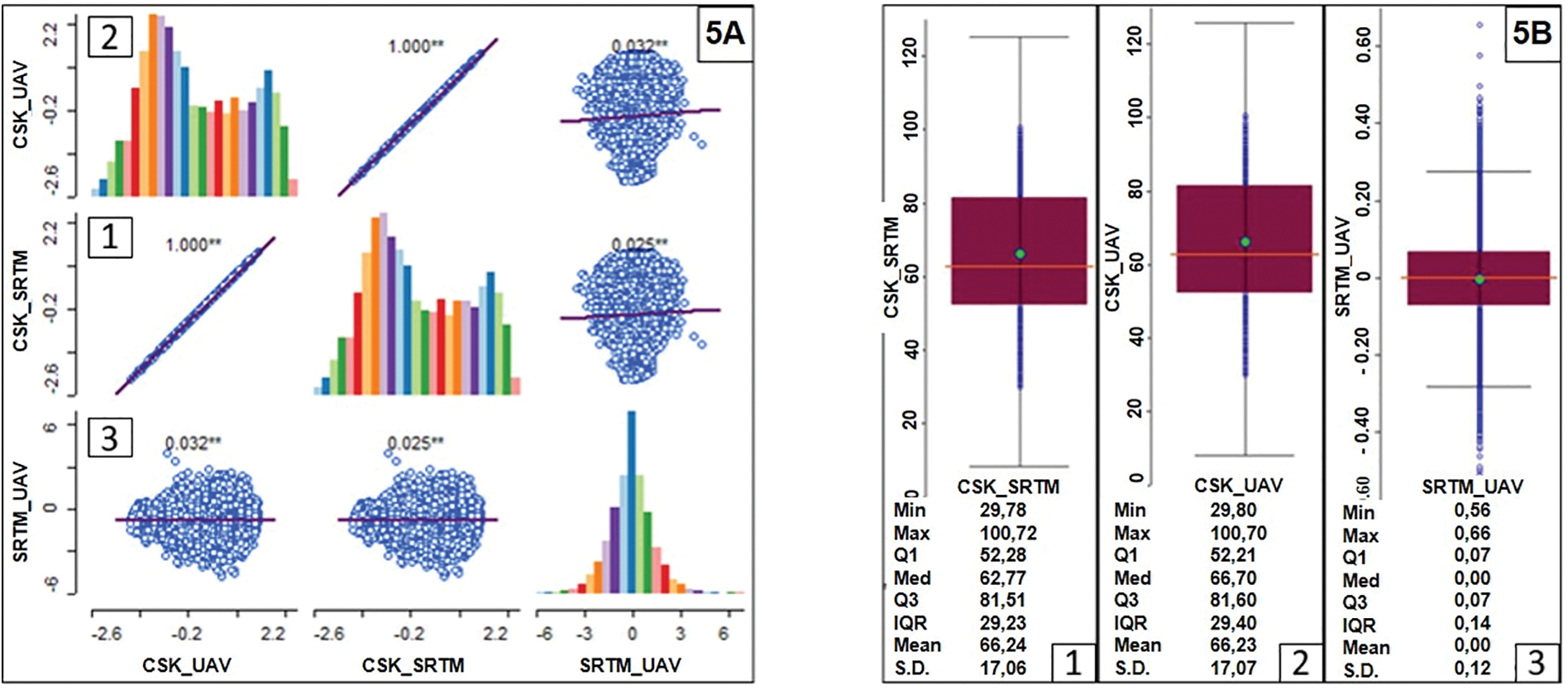
Figure 5: Distributions and spatial relationships of elevation differences: CSK-SRTM, CSK-UAV and SRTM-UAV

3.5 Elimination of Outlier Changes in the Rates of Spatial Variation in Elevation with Bayer’s Approach

Fig. 6A shows the rate of raw variations, obtained with an intrinsic empirical variance instability, before the removal of false changes. To correct for outliers, the empirical Bayes smoothing and spatial averaging approaches were combined. Fig. 6B shows the improved result. Which specifies the height variations from the raw rate, having borrowed strength from the other observations, after imputing the matched difference standard deviation to the latter, following the logic of the syntaxes given in the previous section.

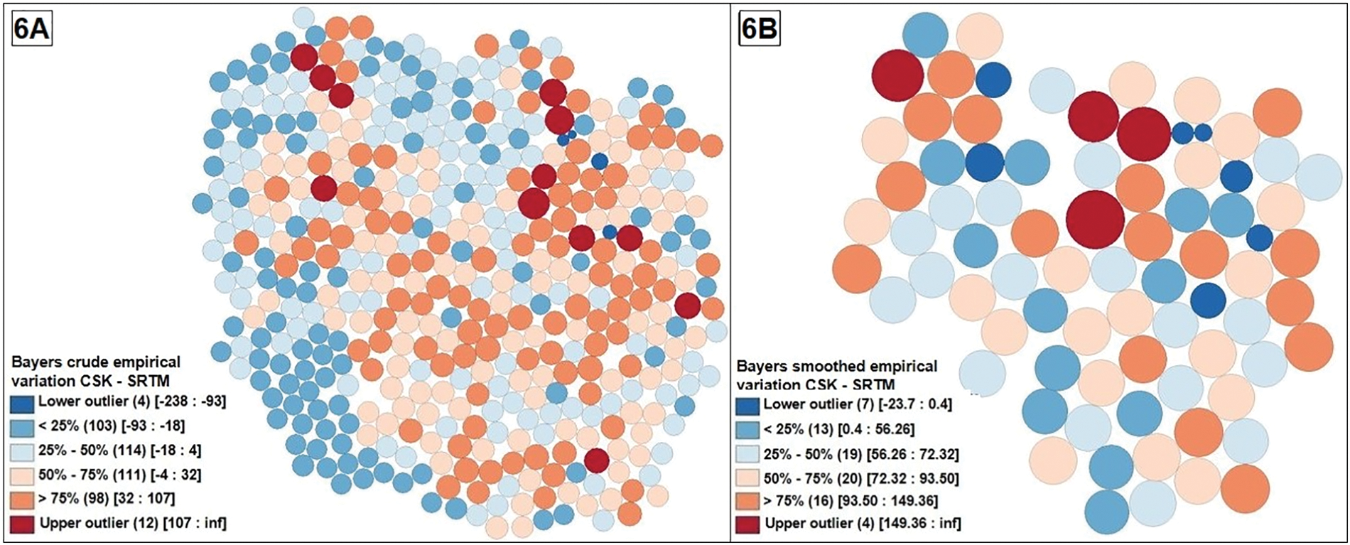
Figure 6: A: Raw elevation changes for the 442 geodetic markers. B: Smoothed elevation changes on the geodetic markers after removing outliers and taking into account standard deviations of paired differences

3.5.1 Elimination of Outlier Changes on Geodesy Markers from Bivariate Moran Scatterplots

Elevation variations at the geodetic marker locations, whatever their order in the geodetic network, are characterized by a positive spatial association. See Figs. 7A (before removal of outliers) and 7B (after removal of uncertain altimeter changes), below. The highly significant slopes of 0.93 and 0.89 are respectively oriented from low-low to high-high on the scatter plots of the point clouds that analyze the altimeter variations at the geodetic marker locations. This positive spatial association increases significantly from the outside to the inside of the KCB, since after eliminating observations of outlier elevation changes, 65.7% of significant topographic variations are found there (Fig. 7F).

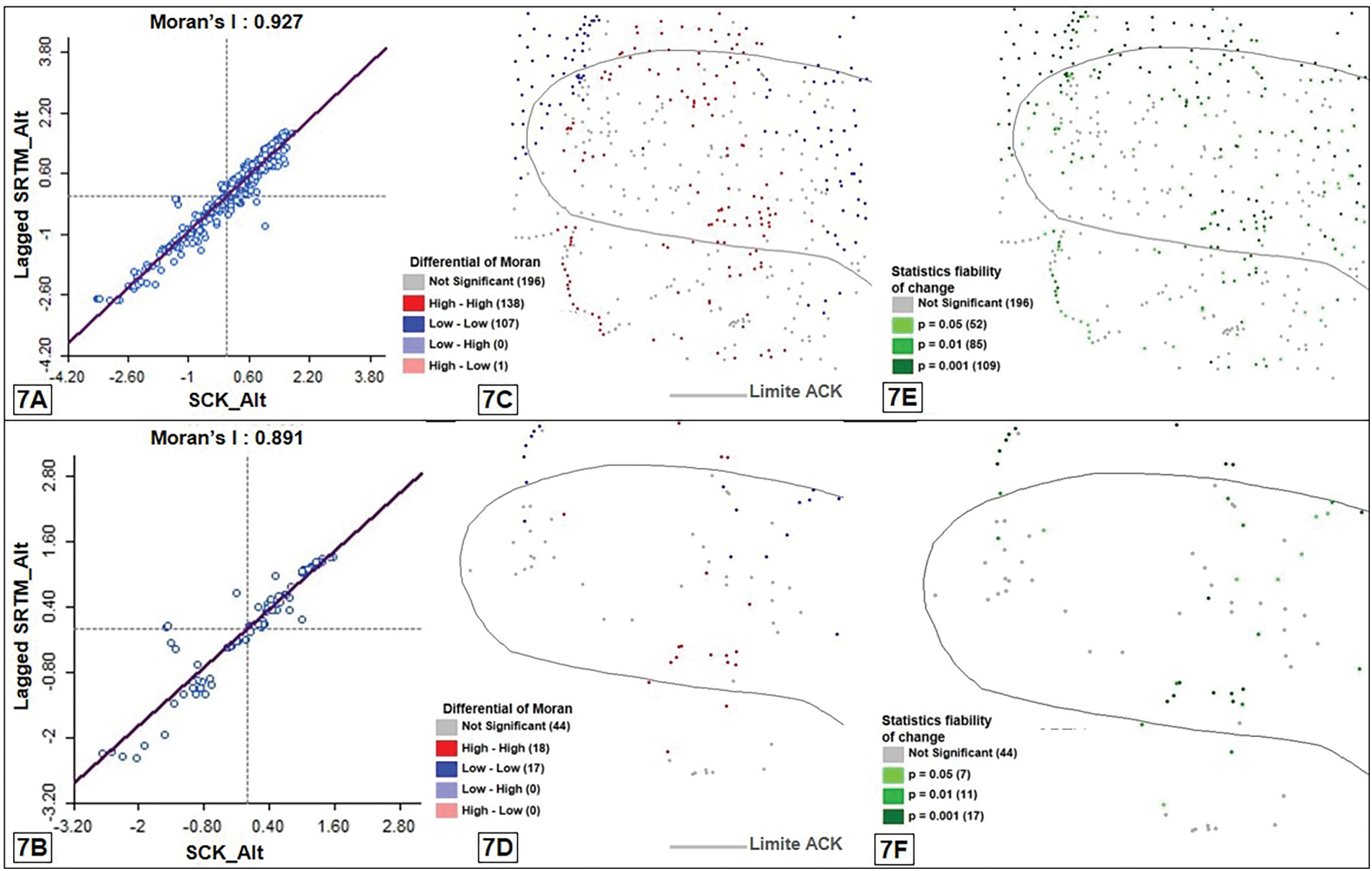
Figure 7: Results of bivariate analyses of the disparity in elevation change. A, C and E: give the dispersion, its statistical significance and the mapping of the topographic change on the geodetic benchmarks, obtained from the analysis of the 442 points before extracting the differences (CSK-SRTM) the error margins calculated for each order of the geodetic markers. B, D and F provide the same analysis as A, C and E, but calculated from the 79 observations from the 442 points, having shown variations after subtraction of standard deviations

The study has retained the best results provided by Figs. 7B, 7D and 7F. A typical elevation variations at the geodetic benchmark locations are observed in the low-high and high-low quadrants (7B). In the first quadrant we note the change in elevation without the significant spatial association of −187.32 m at a first order benchmark (Kyangwale) and two other second order benchmarks: Kyangwale N-E with −159.38 m and Mulunda −73.68 m. The second contains a single similar variation on a third-order marker: Kapidi (62.17 m).

The top-top and bottom-bottom quadrants contain all 35 markers showing spatially significant elevation variations, ranging from −120.48 to 250.68 m. Thus, for the smoothed result (Fig. 7F) at the significance level p = 0.05, 2 bounds are highlighted in the high-high quadrant against 5 in the low-low one. The p = 0.01 confirms changes in elevation on 11 points, 6 of which are in the high-high quadrant and 5 again in the low-low quadrant. As for the p = 0.001, 6 elevation changes of the markers are recorded in the low-low area against 12 others in the high-high area. 44 statistical variations in elevation on the geodetic markers were found to be spatially insignificant in all 79 locations that had previously met the change criteria. The majority of landmark positions varied in relation to the location of extraction and storage of mining or quarrying products.

3.6 Elevation Variation according to the Orders of the Geodetic Markers

Extreme elevation changes are observed on the order 2 marker locations (see Fig. 8), in the two square degrees under study, of the Katanga geodetic network. This coincides with the situations of the mineralized hills, where the series of mines sometimes outcrops in flakes; they constitute the targets for easy exploitation of Cu, Cobalt and Gold ores for some.

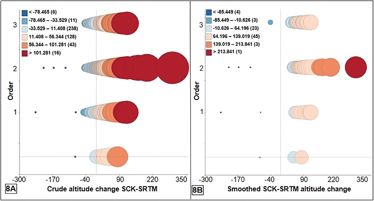
Figure 8: Gross (A) and smoothed (B) variations according to the orders: 1, 2 and 3 of the geodetic markers

3.7 Elevation Variation according to the Orders of the Geodetic Markers

The ratio of about 0.34 characterizes the result grouping the elevation variations. It confirms the spatially very fragmented topographic variations. It reflects both the randomness of the location of the geodetic markers, and the level of disparity of intra-and extra-order changes in the geodetic network, which sometimes rhymes with the geological exceptionally outcrops of the copper-cobalt deposits; generally located on higher ground, at which places there would be geodetic markers in the KCB. Thus, the exploitation of the deposits at the locations of the geodetic markers would be largely responsible for the abrupt change in relief.

We note from the results of the synthesis mapping (Fig. 9) the absence of the 79 geodetic markers in their places. Among them, are three markers of indefinite order; two of them with low probabilities of disappearance or obstruction for one and very high (p = 0.001) for one. Eleven markers of order 1 fail at their locations in the two square degrees of the study area. The probability levels of their absences range from low (7 markers), to medium (1 marker), high (1 marker) to very high (1 marker). As for the second order markers, 35 would be missing at their positions; with respective p’s of: 0.05 (2 markers), 0.01 (6) and 0.001 (7 markers), including the other 20 markers whose probability of absence at their locations is low. Considering the disappearance or obstruction of markers of order 3; 15 are classified in the set of probably weak disappearance, against 4 and 4 having the p respectively of 0.05 and 0.01 and 7 absences of markers found at p = 0.001.

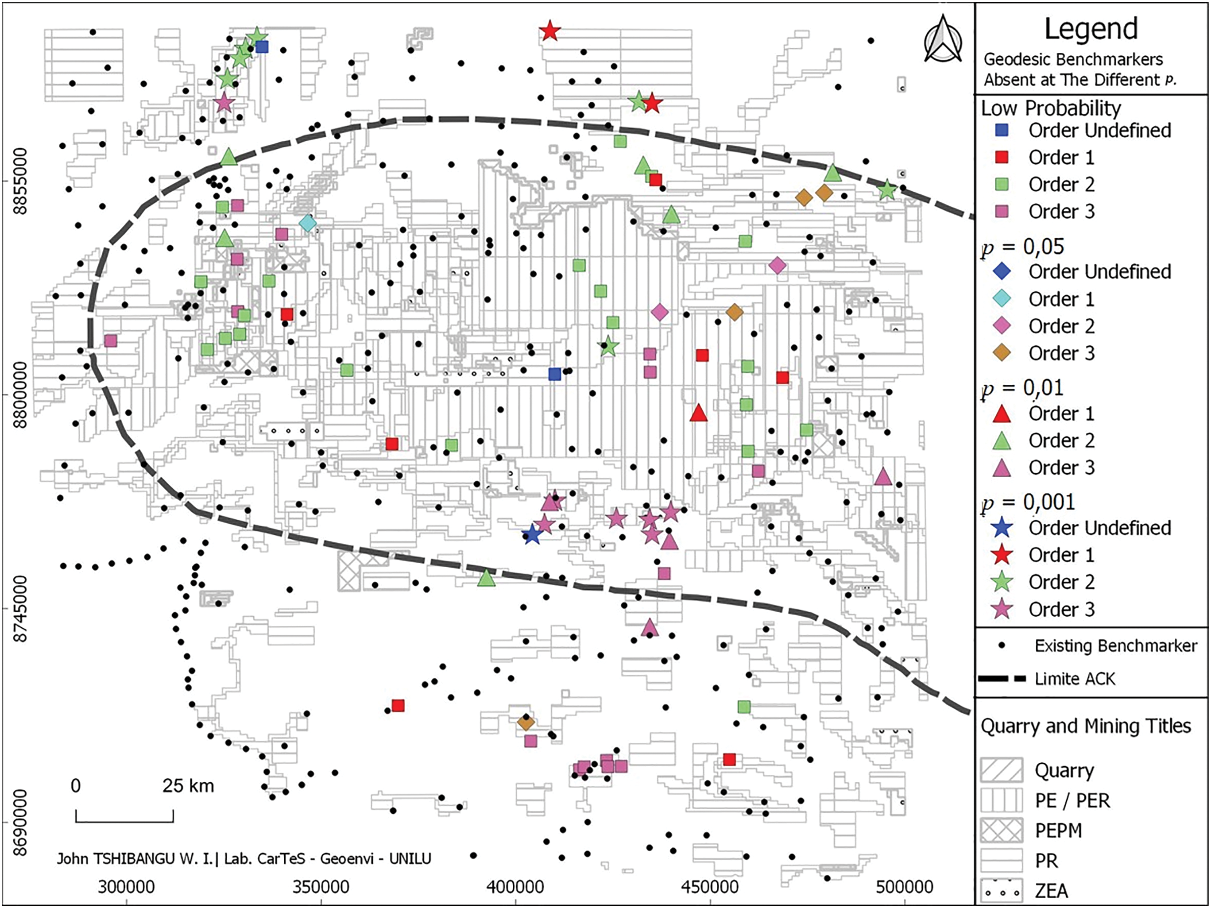
Figure 9: Mapping of the missing or obstruction of geodetic markers with different levels of significance (p). This map provides the situation of the geodetic network from 1912 to 2000

The large loss is observed in the category of benchmarks of order 2, followed by 3. Almost all geodetic benchmarks with a high probability of absence at their locations are found in the KCB, although the exact quantification of the height variation on a geodetic benchmark will require the field survey. This, given that the results of the statistical analysis on the three data sets (CSK, RSTM and UAV) reveal an offset which could be due to differences in the topographic measurement techniques used and the consideration of local datum.

4  Discussion

In Dequincey et al. [46], the authors explained continental mobilism by the bimodal distribution of global elevations. However, in the present study, the asymmetric distribution of the CSK and SRTM data sets allowed us to understand that the geodetic benchmarks are randomly distributed in the study area.

The data and tools exploited in this paper are adapted to the need for analysis and characterization of macro-change in relief and inventory of geodetic landmarks. The performance of SRTM proves to be an appropriate response to this need. The average CSK-SRTM height errors were respectively: 12.6594, 13.3796 and 7.3369 m, depending on orders 1, 2 and 3. These values are very close to the vertical root-mean-square error (RMSE) of ±12.526 m obtained by Ibrahim et al. [47] when evaluating a Digital Elevation Model (DEM) derived from contour lines (CL) against the DEM from an aerial photo. And even, by 8, 10.14, and 14.38 m which were respectively established by Mukul et al. [48] as the RMSE of elevations of SRTM data calculated from the bands: X and C of one arc and C of 3 arcs. The study by Bourgine et al. [49] found the standard deviation of the error to be around 10 m by examining the altimetric accuracies of SRTM, airborne laser, helicopter-borne DTM datasets, and IGN dimensioned points in Cayenne, French Guiana.

The differences in standard deviations of: 40.411 m (SRTM), 42.332 m (Google Earth) and 43.383 m (ASTER GDEM 2) were recorded by Ibrahim et al. [47] when analyzing the vertical accuracies of the latter datasets in relation to the DEM derived from the LCs. The value of around 16 m was obtained at 90% confidence level by Bourgine et al. [49], deviating from those established by the advanced statistical analysis of our study. At 99.99% confidence intervals, the respective elevation differences of: 38,868, 25,586 and 20,625 m for orders 1, 2 and 3 of the CSK-SRTM data were observed. The results of Kolecka et al. [50] established respectively for the SRTM C and X bands mean errors equal to 4.31 ± 14.09 and 9.03 ± 37.40 m and root-mean-square errors equal to 14.74 and 38.47 m, close to results shown in our study. And even around 25 m was found by Ferreira et al. [51] in a similar study.

Altimetric accuracy errors increase with decreasing geodetic terminal orders. Ganie et al. [22] found that SRTM vertical inaccuracy was significant at higher elevations (>1500 m) or steep slopes [49,52] recorded differences of 5.61 ± 15.68 m for areas with high relief and sparse tree cover, and 3.53 ± 8.04 m for flat areas with dense vegetation. Observations by Kolecka et al. [50] point in the same direction, with an error due to forest cover of around 10 m. The 1st-order landmarks are located on the very rugged terrain overhanging the study area at high elevations (>1400 m). They show a higher altimetric accuracy error of 38.868 m compared with 25.586 and 20.625 m, respectively for the order 2 and order 3 benchmarks.

The results highlighted in this study show that the data and the methodology used are suitable for identifying major topographic changes. However, they do not allow the detection of minor variations on the landforms bearing the geodetic markers. This limitation could be due to the low spatial resolution of the SRTM image used in the research and to the divergence of reference zeros (local CSK zero and global SRTM zero). This last argument is confirmed by the small difference between the SRTM (2000) and UAV (2021) data in Fig. 5A. However, the UAV point clouds were collected with a pixel resolution of the order of one meter in contrast to the SRTM data which had 30 m. It is understood that the similarity of the variables in the SRTM and UAV data sets is related to the similar positioning technologies used to acquire the latter data.

The discrepancy between CSK, SRTM and UAV data is thought to be due to the penetrating power of the SRTM C and X bands, disrupted by strong topographic features and dense forest cover. References [51,53] highlighted the advantage of ALOS PALSAR’s low-frequency L-bands over SRTM’s medium-frequency C-band in object detection. Further study of the evaluation of the respective altimetric sensitivities of low-frequency and hyperspectral radar bands is underway in the CarTeS laboratory to understand the influence of edaphic conditions on the vertical accuracy of data provided by the above-mentioned bands. This would contribute to the question of developing an effective methodology for this.

Normally, it is recommended to proceed with direct field inspection and measurements for such a study, related to the control and management of the geodetic network, carried out through the indirect inventory of the geodetic markers that constitute it. But currently, the emergence of geomatic sciences (remote sensing and GIS) having boosted new collection and analysis techniques of geospatial information that facilitate their processing, raises the growing interest in the scientific community. The aim is to test the reliability of data derived from geospatial techniques and also to identify the methods that would be suitable for their exploitation [42] in order to solve concrete problems in society.

5  Conclusion

This work analyzed the state of the geodetic network in an area of heavy mining and forestry, based on CSK (1919–1952) and SRTM (2000) data, arbitrated by the UAV survey carried out in 2021. We have indirectly inventoried the completeness of the existing geodetic monuments and deduced the evolution of the relief in the N-W part of the KCB. The research finds that in the two square degrees under study, on the 442 markers of the geometric and trigonometric triangulation network, 79 markers are missing in their places. With confidence levels varying between p 0.05 and p 0.001. The majority of this loss coincides with the locations of quarrying and mining activities in the KCB and its surroundings.

With this in mind, the present contribution has set out on the one hand to find a method for testing the reliability of SRTM data by comparing them with the topographic data collected by the CSK in the southern part of the DRC. On the other hand, to find a way to remotely monitor the situation of the geodetic network in the KCB. The study proposes a methodological approach applicable to the indexation of major elevation variations at the locations of geodetic markers. Indeed, it is becoming frequent to observe abrupt topographic changes at the locations where geodetic markers are established. In addition, the state institution in charge of the management of the said geodetic network remains without means to play its role.

Acknowledgement: The authors would like to thank the editor and the reviewers for their contribution to the improvement and publication of our paper.

Funding Statement: The authors received funding from CGS SARL for data collection and CarTeS laboratory for technical support.

Author Contributions: The authors confirm contribution to the paper as follows: Project design and data collection were carried out by John Tshibangu W.I. For the work concerning processing, analysis and writing, all the authors participated equally. Catherine Nsiami M. supervised the work.

Availability of Data and Materials: Updated (SRTM, UAV) and historical (CSK) data are stored on the local CarTeS Laboratory server and can be shared with other researchers on request. The digital processing of data was done on the computer using software: Excel, QGIS, SPSS and GeoDa.

Conflicts of Interest: The authors declare that they have no conflicts of interest to report regarding the present study.

1https://www.earthdata.nasa.gov/sensors/srtm

2https://asterweb.jpl.nasa.gov/

3https://www.eorc.jaxa.jp/ALOS/en/dataset/aw3d30/aw3d30_e.htm

4https://data.europa.eu/data/datasets/5eecdf4c-de57-4624-99e9-60086b032aea?locale=en

References

1. Kabulu DJP. Evaluation et cartographie de la déforestation au Katanga (Mémoire de DEA). Bruxelles : Unversité Librede Bruxelles; 2006. [Google Scholar]

2. Cabala Kaleba S, Sikuzani Useni Y, Sambieni KR, Bogaert J, Kankumbi Munyemba F. Dynamique des écosystèmes forestiers del’Arc Cuprifère Katangaisen République Démocratiquedu Congo. I. Causes, transformations spatiales et ampleur. Tropicultura. 2017;35(3):192–202. [Google Scholar]

3. Soyer J, Wilmet J. Etude de l’environnement de Lubumbashi de 1973 à 1981 à l’aide de la télédétection par satellite : croissance urbaine et déboisement. Geo-Eco-Trope. 1983;7(1–4):67–81. [Google Scholar]

4. Malaisse F, Batubenga K, BIzangi K, Ipanga T, Kakisingi M. Essai cartographique sur l’environnement et sa dynamique en milieu tropical humide : les moyens plateaux de Shaba méridional. Geo-Eco-Trope. 1983;7(1–4):49–65. [Google Scholar]

5. Bizangi K. Contribution à l’étude du déboisement en Afrique Tropicale : Le cas du Shaba méridional. Lubumbashi : Université de Lubumbashi; 1988. [Google Scholar]

6. Dikumbwa N, Tshibang Nawej S, Malaisse F. Vie et lente agonie d’une colline de cuivre du Haut-Katanga : la colline de Luiswishi. Geo-Eco-Trop. 2022;46(1):1–14. [Google Scholar]

7. Straeten VDJ. Triangulation du Katanga. Les Bases géodésiques (en général). Mesure de la base de Gandajika. Bulletin de l’Institut Royal Colonial Belge, tome; XX, fasc.4 (G.S.K., op. 16 des Publications relatives à la Cartedu Katanga.) ; 1949. [Google Scholar]

8. Straeten VDJ. Tronçons XIII à XVII de la triangulation fondamentale et groupes X à XIV du nivellement trigonométrique général. Académie Royale des sciences Coloniales Belge, classe des sciences techniques, mémoiresin-8°. Nouvelle série, Tome I, fascicule 4 et dernier. 1955. [Google Scholar]

9. Kulemin GP, Lukin VV, Zelensky AA, Kurekin AA, Engman ET (1997). Radar dual-polarization remote sensing of soil erosion. Proceedings of SPIE 3222, Earth Surface Remote Sensing. doi:10.1117/12.298141. [Google Scholar] [CrossRef]

10. Shmilovitz Y, Marra F, Wei H, Argaman E, Goodrich D, Assouline S, et al. Assessing the controlling factors on watershed soil erosionduring intense rainstorm eventsusing radar rainfall andprocess-based modeling. Catena. 2023;231:107282. doi:10.1016/j.catena.2023.107282. [Google Scholar] [CrossRef]

11. Massonnet D, Kurt LF. Radar interferometry and its application to changes in the Earth’s surface. Rev Geophys. 1998;36(4):441–500. doi:10.1029/97RG03139. [Google Scholar] [CrossRef]

12. Dean BG, Sandra P, Worstell BB. Vertical land change in select counties of Kentucky, Minnesota, and Wisconsin. U.S. Geological Survey Data Release. 2017. doi:10.5066/F7445K05. [Google Scholar] [CrossRef]

13. Zandbergen P. Applications of shuttle radar topography mission elevation data. Geogr Compass. 2008;2:1404–31. doi:10.1111/j.1749-8198.2008.00154.x. [Google Scholar] [CrossRef]

14. Yang LP, Meng XM, Zhang XQ. SRTM DEM and its application advances. Int J Remote Sens. 2011;32(14):3875–96. doi:10.1080/01431161003786016. [Google Scholar] [CrossRef]

15. Gesch DB. An inventory of topographic surface changes: the value of multitemporal elevation data for change analysis and monitoring. Int Arch Photogramm, Remote Sens Spat Inf Sci. 2014;XL-4:59–63. doi:10.5194/isprsarchives-XL-4-59-2014. [Google Scholar] [CrossRef]

16. Kumar Rana V, Suryanarayana TMV. Visual and statistical comparison of ASTER, SRTM, and Cartosat digital elevation models for watershed. J Geovis Spat Anal. 2019;3(2):12. doi:10.1007/s41651-019-0036-z. [Google Scholar] [CrossRef]

17. Patel PP, Sarkar A. Terrain characterization using SRTM data. J Indian Soc Remot Sens. 2021;38:11–24. doi:10.1007/s12524-010-0008-8. [Google Scholar] [CrossRef]

18. Orengo HA, Petrie CA. Multi-scale relief model (MSRMa new algorithm for the visualization of subtle topographic change of variable size in digital elevation models. Earth Surf Process Land. 2018;43:1361–9. doi:10.1002/esp.4317. [Google Scholar] [PubMed] [CrossRef]

19. Gaye HK. Gestion du réseau géodésique national (Mémoire de fin d’étude). Ouagadougou : Groupe des écoles EIER-ETSHER; 2004. [Google Scholar]

20. Desbois H. Les mesures du territoire : Aspects techniques, politiques et culturels des mutations de la carte topographique. vol. 1. Villeurbanne: Pressesdel’enssib; 2015. [Google Scholar]

21. Maniere L. Extraction d’informations topographiques et hydrologiques à partir d’un modèle numérique de terrain – Cas pratique sur le MNT du projet desert networks. 2019. Available from: https://desertnetworks.hypotheses.org/920. [Accessed 2022]. [Google Scholar]

22. Ganie PA, Posti R, Aswal AS, Bharti VS, Sehgal VK, Sarma D, et al. A comparative analysis of the vertical accuracy of multiple open-source digital elevation models for the mountainous terrain of the north-western Himalaya. Model Earth Syst Environ. 2023;9(2):2723–43. doi:10.1007/s40808-022-01641-x. [Google Scholar] [CrossRef]

23. Dikumbwa N, Mbenza Mwana A. Flore des anomalies géobotaniques de la ceinture cupro-cobaltifère du Katanga méridional. Les spécificités biotopiques par le coefficient de recouvrement et le degré de sociabilitédesphytotaxons. Geo-Eco-Trope. 2021;45(4):529–40. [Google Scholar]

24. Lerat S. Une région industrielle au cœur del’Afrique : Le Katanga méridional. Cahiers d’outre-Mer, N° 56-14ème année. 1961;435–42. [Google Scholar]

25. Cornet J. Les richesses minières du Congo Belge. Encyclopédie du Congo belge. Bielleveld; 1982. [Google Scholar]

26. Robert M. Contribution à la géologie du Katanga : Le système du Kundelungu et le système Schistodolomitique. Belgique : Institut Royal Colonial Belge, sectiondes sciences naturelles et médicales; 1940. [Google Scholar]

27. Armand F. La structure tectonique du Katanguien dans la région de Kolwezi (Shaba, Rép. du Zaïre). Annales de la Société Géologique de Belgique, Fascicule 1. 1993;116:87–104. [Google Scholar]

28. Cailteux J. Le Roan Shabien dans la région de Kambove (Shaba-Zaïre) (Thèse de doctorat). Université de Liège : Liège; 1983. [Google Scholar]

29. Kampunzu AB, Cailteux J. Tectonic evolution of the Lufilian Arc (Central Africa copper belt) during Neoproterozoic pan African Orogenesis. Int Assoc Gondwana Res, Japan. 1999;2(3):441–44–21. [Google Scholar]

30. Maury J. Triangulation du Katanga. Tome I, fascicule 1. Belgique: Institut royal colonial Belge, sectiondessciences techniques, mémoires; 1930. [Google Scholar]

31. Straeten VDJ. Mesure des bases de Kilambo et de Pweto. Bulletin De l’institut Royal Colonial Belge. 1930;tome I, fasc.3:566–610. [Google Scholar]

32. Gilliard AA. Cartographie congolaise. Mémoires-Collection in n°8 Tome IX, fasc. 1. Section des scienceset techniques, institut royal colonial belge; 1955. [Google Scholar]

33. Gilliard AA. Cartographie congolaise. Collection in-8°. Tome IX, fascicule 1. Belgique : Institut royal colonial Belge, section des sciences techniques, mémoires; 1955. [Google Scholar]

34. Rezgui M, Ben Hadj Salem A. Theory of errors for technical assistants working in the field of surveying and topography. Version 1.0. 2021. Available from: https://www.researchgate.net/publication/356814984_Notions_of_The_Theory_of_Errors_For_Technical_Assistants. [Accessed 2022]. [Google Scholar]

35. Derrick B, Ruck A, Toher D, White P. Tests for equality of variances between two samples which contain both paired observations and independent observations. J Appl Quant Methods. 2018;13(2):19. [Google Scholar]

36. Simon LJ. Estimateur de Stein, régularisation et pénalisation. Apprentissage : Cours 10; 2014. [Google Scholar]

37. Anselin L. Cartes pour les taux ou les proportions. 2018. Available from: https://geodacenter.github.io/workbook/3b_rates/lab3b.html. [Accessed 2022]. [Google Scholar]

38. Levene H. Contributions to probability and statistics: essays in honor of harold hotelling. Palo Alto: Stanford University Press; 1960. p. 278–92. [Google Scholar]

39. Brown B, Forsythe AB. Robust tests for the equality of variance. J Am Stat Assoc. 1974;69:364–7. [Google Scholar]

40. Lee SI. Développement d’une mesure d’association spatiale bivariée : uneintégration du r de Pearson et du I de Moran. J Des Syst Géogr. 2001;3:369–85. [Google Scholar]

41. Ertur C, Koch W. Analyse spatiale des disparités régionales dans l’Europe élargie. Laboratoire d’économie etdegestion (LEG); 2004. [Google Scholar]

42. Zaninetti JM. Statistiques de produit croisé pour l’analyse spatiale exploratoire. Cybergeo : Revue Européenne de Géographie. 2007;22(397). doi:10.4000/cybergeo.11203. [Google Scholar] [CrossRef]

43. Duque JC, Richard LC, Middleton RS. The p-regions problem. Geogr Anal. 2011;43:104–26. doi:10.1111/j.1538-4632.2010.00810.x. [Google Scholar] [CrossRef]

44. Anselin L. Autocorrélation spatiale globale (2). Diagramme de dispersion de Moran bivarié, différentiel et taux EB. 2019. Available from: https://geodacenter.github.io/workbook/5b_global_adv/lab5b.html. [Accessed 2022]. [Google Scholar]

45. Anselin L. Analyse exploratoire des données (2). Exploration multivariée. 2020. Available from: https://geodacenter.github.io/workbook/2b_eda_multi/lab2b.html. [Accessed 2022]. [Google Scholar]

46. Dequincey O, Thomas P. Distribution bimodale des altitudes et mobilité horizontale (dérive) des continents. 2011. Available from: https://planet-terre.ens-lyon.fr/ressource/distribution-bimodale-altitudestectonique-plaques.xml. [Accessed 2022]. [Google Scholar]

47. Ibrahim M, Al-Mashaqbah A, Koch B, Datta P. An evaluation of available digital elevation models (DEMs) for geomorphological feature analysis. Environ Earth Sci. 2020;79(336):13. doi:10.1007/s12665-020-09075-3. [Google Scholar] [CrossRef]

48. Mukul M, Srivastava V, Mukul M. Accuracy analysis of the 2014–2015 global shuttle radar topography mission (SRTM) 1 arc-sec C-band height model using international global navigation satellite system service (IGS) network. J Earth Syst Sci. 2016;125(5):909–17. doi:10.1007/s12040-016-0716-8. [Google Scholar] [CrossRef]

49. Bourgine B, Baghdadi N. Assessment of C-band SRTM DEM in a dense equatorial forest zone. C R Geosci. 2005;337(14):1225–34. doi:10.1016/j.crte.2005.06.006. [Google Scholar] [CrossRef]

50. Kolecka N, Kozak J. Assessment of the accuracy of SRTM C- and X-band high mountain elevation data: a case study of the polish tatra mountains. Pure Appl Geophys. 2014;171(6):897–912. doi:10.1007/s00024-013-0695-5. [Google Scholar] [CrossRef]

51. Ferreira ZA, Cabral P. A comparative study about vertical accuracy of four freely available digital elevation models: a case study in the Balsas river Watershed, Brazil. ISPRS Int J Geo-Inf. 2022;11(2):106. doi:10.3390/ijgi11020106. [Google Scholar] [CrossRef]

52. Carabajal CC, Harding DJ. ICESat validation of SRTM C-band digital elevation models. Geophys Res Lett. 2005;32(22). doi:10.1029/2005GL023957. [Google Scholar] [CrossRef]

53. Xiong S, Muller JP, Li G. The application of ALOS/PALSAR InSAR to measure subsurface penetration depths in deserts. Remote Sens. 2017;9(6):638. doi:10.3390/rs9060638. [Google Scholar] [CrossRef]