Observation Parameter Selection and Long Integration Time Effect Evaluation for Moon-Based SAR in Polar Sea Ice Monitoring: A Ground-Based Scattering Experiment

1  Introduction

Lunar exploration has increased in recent years, including that of Artemis, Chang’e, Luna, and Chandrayaan. Moon-based Earth observations were explored decades ago for manned lunar landings. During the Apollo 16 mission in 1972, a far-UV telescope was placed on the Moon to capture a picture of the Earth [1]. However, existing studies in this field mostly remain at the theoretical simulation stage, focusing on Moon-based Earth observation geometric characteristic analysis [2], Earth’s radiation measurement simulation [3], land surface temperature retrieval [4], and Moon-based Synthetic Aperture Radar (SAR) capability evaluation [5–7].

The capability of Moon-based SAR for Earth observations has been demonstrated in several studies. These studies mainly focus on the Moon-based SAR imaging capability [5,6], spatiotemporal coverage of Moon-based SAR, spatial baseline for Moon-based SAR cross-track interferometry, and evaluation of ionospheric delay for Moon-based repeat-pass InSAR. Compared with polar-orbiting SAR, Moon-based SAR exhibits some peculiar characteristics. Moon-based SAR can image a large ground swath and even achieve a quasi-global scene by steering the antenna in elevation. For a certain place on Earth, the revisit time of Moon-based SAR can be as short as one day. A high resolution is achievable owing to the long integration time of Moon-based SAR. Moon-based SAR achieves imaging as the Earth rotates, in a manner similar to sliding-spotlight SAR. However, Moon-based SAR has some limitations. First, to achieve both high resolution and a large swath, large antennas are necessary to compensate for the power budget. Second, track curvature could pose challenges to focusing and range migration algorithms. Third, the long integration time could lead to defocusing or decoherence of moving targets on land and in the oceans.

Some Earth observation targets have been suggested for Moon-based SAR, such as global vegetation, solid Earth tides, and sea ice in polar regions. Sea ice plays a crucial role in Earth’s systems, especially in global climate regulation [8]. In our previous study, the Moon-based spatial coverage and observation time for sea ice in polar regions were studied, which suggested that the Antarctic Marginal Ice Zone (MIZ) could be a potential phenomenon for Moon-based Earth observations [9].

However, Moon-based SAR imaging and sea ice scattering have not yet been studied. Moon-based SAR has several characteristics that differ from spaceborne SAR, such as the longer integration time [5] and larger incidence angles for observation in polar regions. To determine whether Moon-based SAR characteristics can affect sea ice detection from the perspective of scattering and imaging, a ground measurement experiment was conducted. On one hand, this experiment was conducted to determine the Moon-based SAR parameters suitable for sea ice monitoring, mainly polarizations and incidence angles. On the other hand, it aims to observe the imaging characteristics of water fluctuation and its effect on sea ice imaging under a long integration time. Unlike most previous research, which has relied on theoretical simulation, this study is innovative in using laboratory experimentation to simulate the characteristics of Moon-based Earth observations. This is the first time that the scattering performance of ice and water has been achieved in an experiment under certain Moon-based SAR imaging characteristics. This study represents a step toward demonstrating the capability of Moon-based SAR for sea ice detection.

The remainder of the paper is structured as follows: Section 2 describes the experiments and data; Section 3 introduces the dissimilarity measures for ice–water discrimination; Section 4 presents the results and discussion; finally, Section 5 concludes the study.

2  Experiment and Data

The experiment was conducted in January 2024 at the Laboratory of Target Microwave Properties (LAMP), in Zhejiang Province. This laboratory has an indoor experimental platform for measuring the microwave characteristics and simulating targeted imaging. The internal structure of the laboratory was 24 m long, 24 m wide, and 17 m high. This can provide experimental conditions for research on microwave remote sensing, such as the verification of the electromagnetic scattering theory model and research on the mechanism of target electromagnetic scattering.

Side and top views of the platform are shown in Fig. 1. The experimental scenarios are illustrated in Fig. 2. Ice-water mixing scenarios were set up to simulate the sea ice scene in polar regions. The ice floats in saline water were placed in a rectangular container 160 cm long, 120 cm wide, and 50 cm deep. The water depth was 45 cm. Before and after the experimental measurements, the temperature and humidity values of the microwave anechoic chamber need to be recorded at least twice a day. If the temperature change of air exceeds 5°C, or the humidity change exceeds 5%, the constant temperature and humidity system needs to be activated to control the environmental temperature and humidity until they meet the measurement requirements.

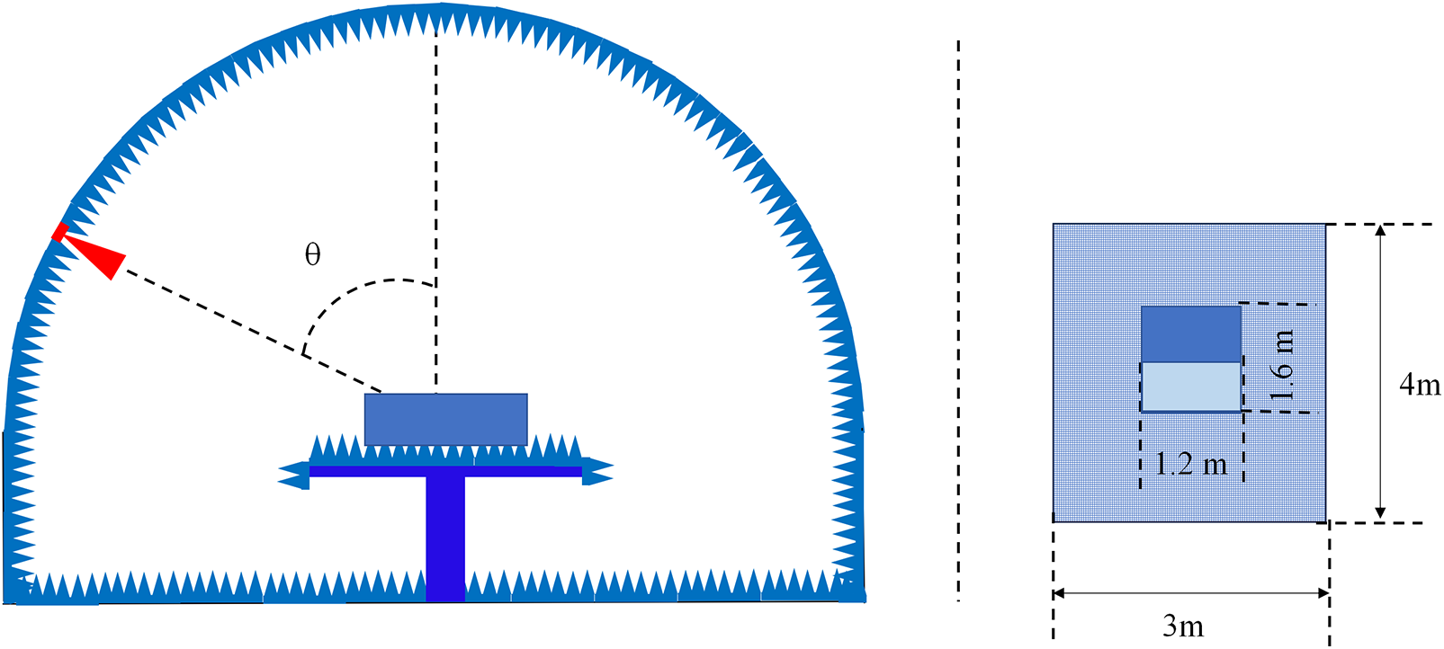
Figure 1: Side and top views of the platform.

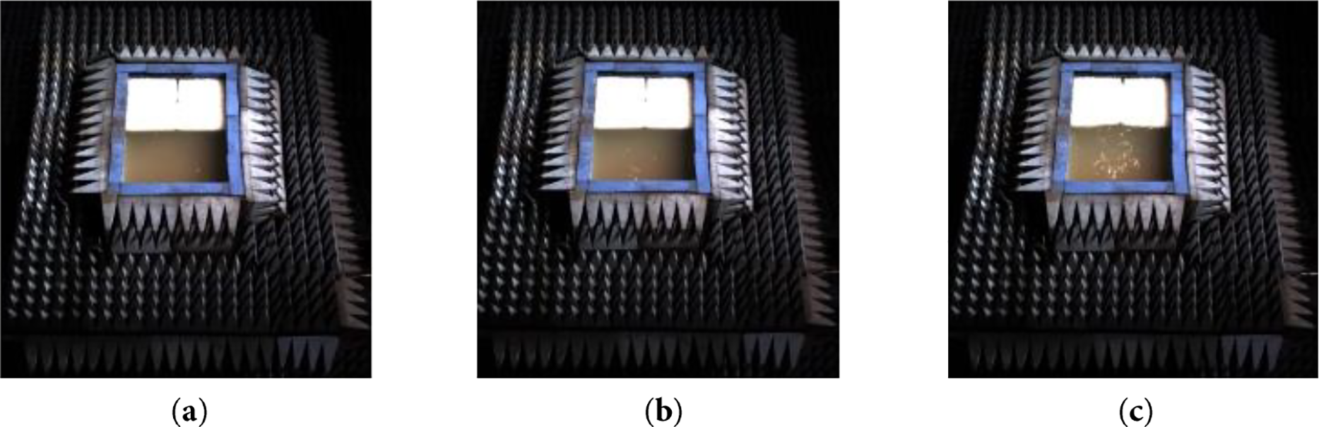
Figure 2: Scene layouts of (a) Calm water, (b) Slightly rough water and (c) Highly rough water.

The imaging radar used in this experiment has some features in common with Moon-based SAR. First, imaging in this experiment was achieved using an inverse SAR (ISAR). In ISAR, the image is obtained by utilizing the motion of the target. As the target moves, the radar captures multiple signals at different angles to create high-resolution images. Moon-based SAR achieves imaging as the Earth rotates. As the Earth rotates, a target on the Earth moves, and the radar on the moon is able to capture multiple signals to create images. Therefore, the imaging mode used in this experiment was similar to that of the Moon-based SAR. Second, the integration time in this experiment was 283 s, which is much longer than that of typical spaceborne SAR, e.g., 0.7 s for ASAR. The integration time of the C-band Moon-based SAR is several minutes [5]. Therefore, the integration time in this experiment was close to that of the Moon-based SAR in magnitude (minutes). Third, large incidence angles were set to simulate the Moon-based SAR observation geometry of the polar regions.

This experiment was conducted to determine the Moon-based SAR parameters suitable for sea ice monitoring, mainly polarizations and incidence angles. C-band quad-polarization SAR data were acquired at an incidence angle range of 30°–70°. The center frequency was 5.3 GHz. The bandwidth was 2 GHz. The frequency interval was set at 50 MHz. The range resolutions at incidence angles of 30°, 40°, 50°, 60°, and 70° were 0.15, 0.12, 0.10, 0.09, and 0.08 m, respectively. The azimuth resolutions at incidence angles of 30°, 40°, 50°, 60°, and 70° were 0.08, 0.06, 0.05, 0.05, and 0.04 m, respectively. C-band satellites have been used extensively for the operational monitoring of Arctic sea ice [10]. The incidence angle range was set to 30°–70° because the Moon-based Earth observation geometry revealed that incidence angles of 27°–72° and 27°–60° are necessary to fully cover the sea ice in the Arctic and Antarctic, respectively. However, according to theory, the backscatter of ice and water at large incidence angles may be too weak, resulting in a low signal-to-noise ratio. This experiment was conducted to evaluate the backscattering performance of ice and water at large incidence angles.

The experiment also observed the imaging characteristics of water fluctuation and its effect on sea ice imaging under a long integration time. A wave pump was used to generate the fluctuating water conditions. Three water conditions were used for imaging in the experiment: calm water, slightly rough water, and highly rough water. Artificial sea ice was prepared. The water salinity was 35‰, close to the salinity of the Southern Ocean [11]. The artificial sea ice was made by freezing artificially adjusted saline water (24‰) [11] in a refrigerator for 5 days at −40°C. After 5 days, the salinity of the ice surface was approximately 11‰, which is within the surface salinity range of the first-year ice (FYI), the dominant sea ice type in the polar regions [12,13]. A single ice block was approximately 56 cm long, 35.5 cm wide, and 13 cm thick. To control ice surface roughness, small ice cubes with a side length of 2 cm were spread on the surface of the ice block. This method was developed by Bredow and Gogineni [12]. The ice surface roughness parameters were as follows: the root mean square height of 0.32 cm and surface correlation length of 1.82 cm.

The experimental platform utilizes three standard calibrators of known dimensions to calculate the calibration coefficients for quad-polarization, and performs relative calibration on the measured data through a quad-polarization calibration coefficient matrix. The SAR images acquired for the three scenarios are shown in Fig. 3. For each scenario, the backscatter of ice and water was acquired and evaluated for the performance of ice–water discrimination for various SAR parameters.

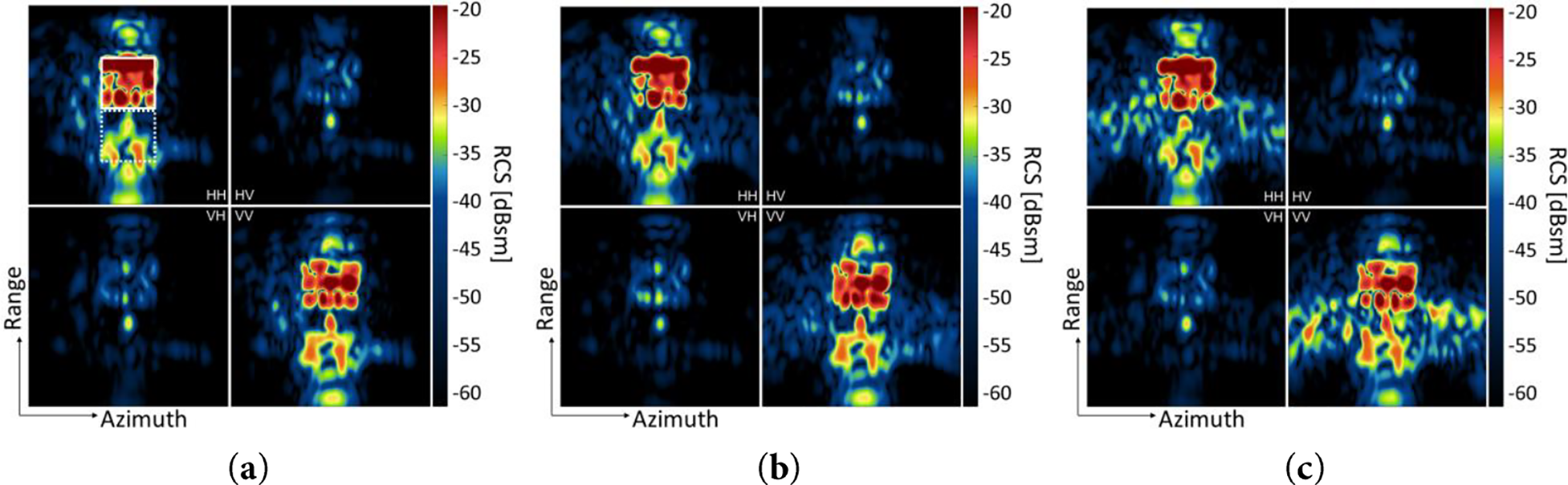
Figure 3: SAR images of ice and water acquired at the incidence angle of 30° for (a) Calm water, (b) Slightly rough water, and (c) Highly rough water. The white solid line box represents ice, and the white dotted line box represents water.

3  Dissimilarity Measures

Dissimilarity measures are used to measure the degree of deviation between data, images, or information. Dissimilarity measure functions can be further divided into categories such as distance measure functions and correlation measure functions. Distance-measurement functions measure the distance between two stochastic processes. Three dissimilarity distance measures were applied: Jensen-Shannon divergence (JSD), Bhattacharyya Distance (BD), and Total Variation Distance (TVD). JSD, BD, and TVD are selected because they are common dissimilarity measurements, but they are not commonly used in ice–water discrimination. In this study, they are used to measure statistical characteristics of ice and water backscatter under a long integration time.

Jensen-Shannon Divergence is a smoothed version of the important divergence measure of information theory, Kullback-Leibler divergence [14]. It is calculated using Eq. (1), and the value ranges are [0,ln⁡2). When the two distributions are identical, the JSD value is zero. When the two distributions are completely nonoverlapping, the JSD value is ln⁡2.

JSD(P,Q)=12∑i=1dpilog⁡(pimi)+12∑i=1dqilog⁡(qimi)(1)

where P and Q are probability distributions, M=12(P+Q), and M is the mixture distribution of P and Q. The samples in P were divided into d parts, and the sample frequency of the i-th part was set as pi. The same procedure was applied to Q and M to obtain qi and mi.

The Bhattacharyya Distance is an often-used measure of distance in statistics and can provide better results than divergence [15]. It is calculated using Eq. (2), and the value range is [0,+∞).

BD(P,Q)=−ln⁡∑i=1dpiqi(2)

The Total Variation Distance is the maximum difference between two probability distributions [16]. It is calculated using Eq. (3), and the value range is [0,1).

TVD(P,Q)=12∑i=1d|pi−qi|(3)

Dissimilarity measures are used to evaluate the degree of deviation between ice and water backscatter, which is the key to sea ice monitoring. Data from the three scenarios were used for the SAR parameter selection. Ice and water samples were manually selected for analysis, as shown in Fig. 3a. The higher the dissimilarity measurement value, the easier it is to distinguish between ice and water. However, it is not possible to determine a fixed threshold for ice–water discrimination based solely on the dissimilarity measurement formula. An effective separability threshold should be provided based on specific data and application scenarios.

4  Results and Discussion

The dissimilarity measurement results for ice and water backscatter are shown in Fig. 4. JSD, BD, and TVD presented different values, but showed similar trends as the incidence angles varied.

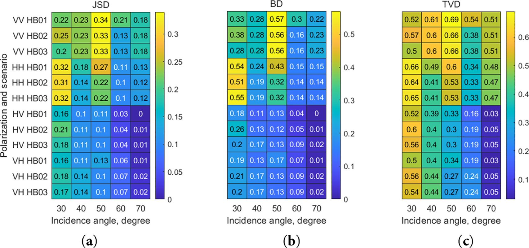
Figure 4: (a) JSD, (b) BD, and (c) TVD values of ice and water backscatter change with incidence angles in quad-polarization, under the calm water (HB01), slightly rough water (HB02), and highly rough water (HB03). The dissimilarity measure value in co-polarization is higher than that in cross-polarization at the same incidence angle within the range of 40°–60°. The dissimilarity measure value in VV polarization is higher than that in HH polarization.

4.1 Parameter Selection: Polarization

At incidence angles of 40°–60°, the dissimilarity measure value in co-polarization (VV and HH) was higher than that in cross-polarization (VH and HV) at the same incidence angle. In co-polarization, the dissimilarity measure value in VV polarization exceeded that in HH polarization; for example, at 50°, JSD was 0.34 for VV compared to 0.27 for HH. This indicates that VV polarization performed better than other polarizations in ice–water discrimination at 40°–60°. At an incidence angle of 30°, HH polarization performed better than the other polarizations in ice–water discrimination. Considering the much higher spatial coverage of sea ice in polar regions by Moon-based SAR at incidence angles of 40°–60° than at 30°, VV polarization is recommended as the preferred polarization for Moon-based SAR under conditions where large antenna quad-polarization is not available.

4.2 Parameter Selection: Incidence Angles

With reference to the noise-equivalent sigma zero (NESZ) in HV polarization RADARSAT-2 images [17], the NESZ in this paper is taken as −30 dB. Therefore, ice backscatter higher than −30 dB is taken as effective. Experimental data showed that incidence angles of 30°–60° provided better ice backscatter, as shown in Fig. 5. In HV polarization, the mean value of ice backscatter at incidence angles of 30°–70° is −25.62, −26.01, −29.17, −29.03, and −33.55 dB, and the standard deviations of ice backscatter at incidence angles of 30°–70° are 6.51, 8.48, 10.19, 9.21, and 8.62 dB. Ice backscatter at the incidence angle of 70° was lower than −30 dB in HV polarization; therefore, 70° was not chosen as an appropriate incidence angle for sea ice monitoring. The HH backscatter incidence angle dependence for sea ice from scenarios HB01, HB02, and HB03 was −0.25, −0.26, and −0.27 dB/° at incidence angles of 30°–60°. The incidence angle dependence value in this experiment was consistent with that of the FYI using spaceborne SAR data [18,19].

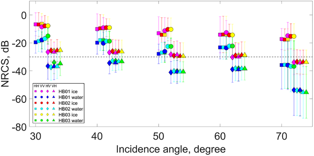
Figure 5: Ice and water backscatter in quad-polarization acquired at the incidence angle range of 30°–70°. Ice backscatters at incidence angles of 30°–60° are higher than −30 dB, which is taken as effective.

In the VV polarization, the dissimilarity measure reached a maximum at an incidence angle of 50°. In the HH, HV, and VH polarizations, JSD, BD, and TVD reached a maximum at an incidence angle of 30°. In co-polarization, the dissimilarity measure values of ice and water backscatter fluctuated with the incidence angles. For example, JSD ranged from 0.21 to 0.34 in the VV polarization under calm water conditions. In cross polarization, the values of the three dissimilarity measures decreased as the incidence angles increased under the three water conditions. For example, the JSD value for the HV polarization ranged from 0.16 to 0.03 with varying incidence angle from 30 to 60°.

4.3 Long Integration Time Effects of Water Fluctuation

Water fluctuation could lead to defocusing in co-polarization owing to the long integration time, but not in cross-polarization, as shown in Fig. 3c. To quantify the defocusing effect, a Fast Fourier Transform was applied to single-look complex data of calm water scenes and highly rough water scenes in the azimuthal direction, and the difference in the Doppler domain was considered to be a change caused by water fluctuation. Using the Inverse Fast Fourier Transform in the spatial domain, the impact of water fluctuations on sea ice imaging can be observed, as shown in Fig. 6. The results showed that the defocusing caused by water fluctuation was mainly distributed along the azimuthal direction and superimposed on the sea ice area, particularly at the ice–water boundary.

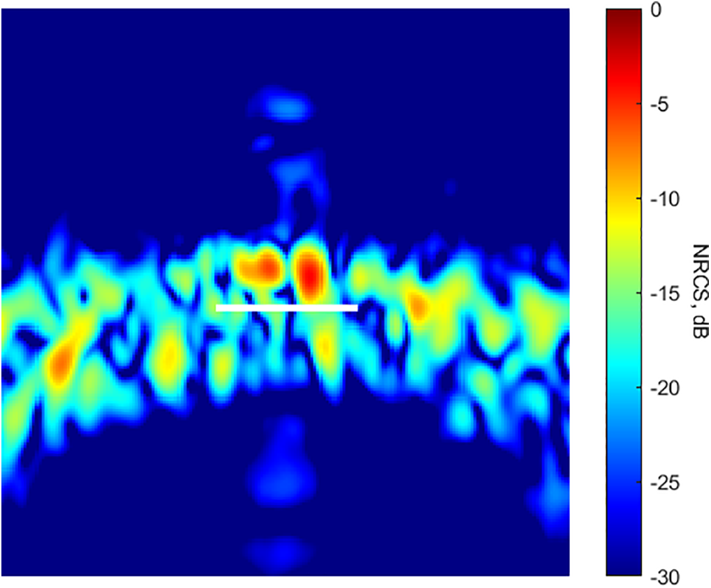
Figure 6: Defocusing effect in VV polarization at an incidence angle of 30° under highly rough water conditions. The white line is the ice–water boundary.

In co-polarization, at incidence angles of 40–60°, water fluctuation caused the dissimilarity measure value of ice and water backscatter to be lower than that under calm water conditions. This can be seen in Fig. 4; for example, at 50°, the JSD was 0.27 for calm water conditions and 0.22 for rough water conditions. This indicates that water fluctuation has a negative effect on ice–water discrimination in co-polarization. In cross-polarization, the dissimilarity measure value in rough water was close to that in calm water, indicating that water fluctuation had little effect on ice–water discrimination in cross-polarization.

To further quantify the degree to which ice and water can be distinguished, the classification accuracy was calculated (Fig. 7). Ice and water were classified using the backscatter threshold. The classification threshold was selected using the following method: first, the probability distribution densities of the backscatter of the ice and water samples were calculated. The intersection point of the two distributions was then considered as the classification threshold. The classification accuracy was defined as the proportion of correctly classified pixels of ice and water. Overall, the classification accuracy showed a trend consistent with the dissimilarity measurement values. In other words, a higher dissimilarity measure value often corresponds to a higher ice–water classification accuracy. In our experiment, to achieve an ice–water classification accuracy higher than 60%, the JSD, BD, and TVD values should be higher than 0.07, 0.09, and 0.24, respectively. To achieve an accuracy greater than 80%, the JSD, BD, and TVD values should be greater than 0.21, 0.26, and 0.6, respectively. Using the same method, each threshold is determined under a specific condition. This threshold determination method is robust. However, thresholds could change under varying noise conditions and water surface states. An effective separability threshold for ice–water discrimination should be determined based on specific data and application scenarios.

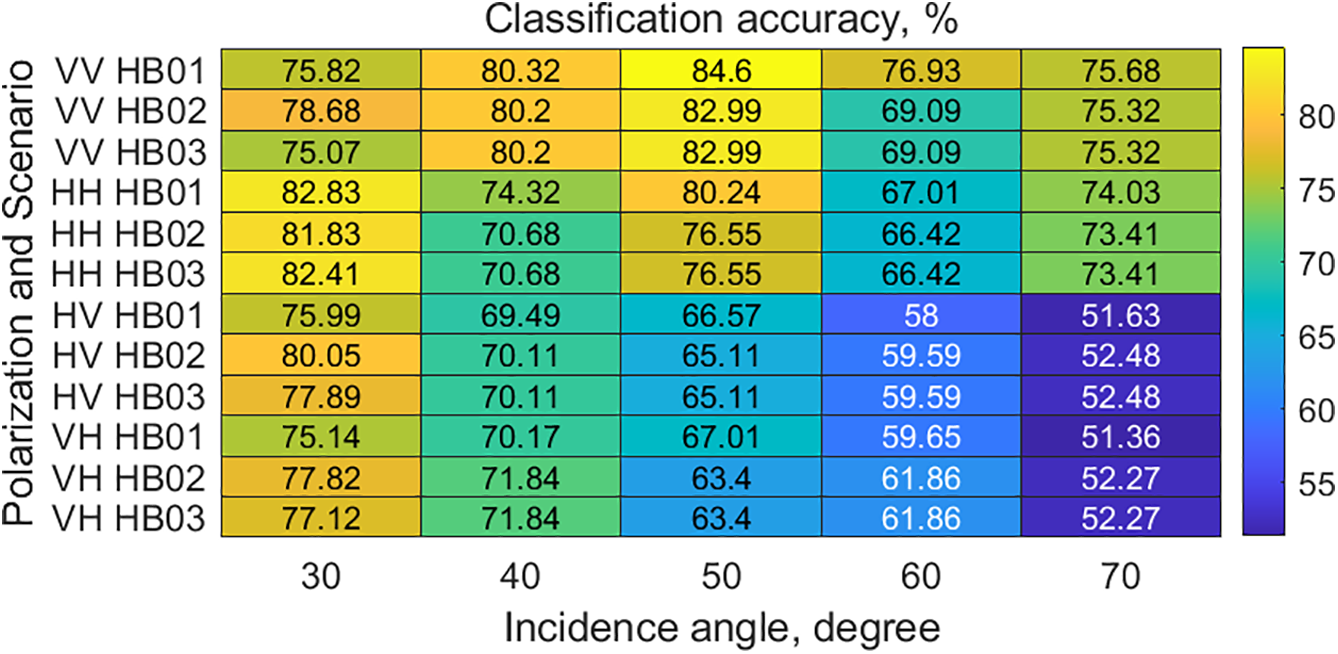
Figure 7: Ice–water classification accuracy based on backscatter at incidence angles of 30°–70° in quad-polarization for three scenarios.

VV polarization achieved a higher ice–water classification accuracy than other polarizations at incidence angles of 40°–60°, while HH polarization achieved higher ice–water classification accuracy than the other polarizations at an incidence angle of 30°. The classification accuracy reached a maximum of 84.60% for VV polarization at an incidence angle of 50° under calm water conditions. At incidence angles of 30°–60°, the ice–water classification accuracy was higher or close to 60% in quad-polarization, whereas the accuracy was lower than 53% at an incidence angle of 70° in HV and VH polarization. While water fluctuation can decrease ice–water classification accuracy by 0.12%–7.84% and 0.42%–3.69% in VV and HH polarization, respectively, accuracies higher than 66.42% can still be achieved. Water fluctuation had no obvious impact on the classification accuracy in the HV and VH polarizations in our experiment. In cross-polarization, the radar system is less sensitive to the surface fluctuations because the signal’s polarization is orthogonal to the surface scattering behavior. Water surface fluctuations typically affect scattering in the same polarization, but cross-polarized signals are more influenced by volume scattering, which is less affected by the direct reflection from the water surface. Therefore, the water surface fluctuations cause less defocusing in cross-polarization because the signal doesn’t rely on the same surface coherence as in co-polarization.

Some of the findings agreed with the well-established SAR scattering behavior, indicating that the scattering characteristics of sea ice do not change over long integration times. These findings offer insights for Moon-based SAR system design. However, certain parameters, such as the orbital height, spatial resolution, signal attenuation over long propagation distances, and geometric distortions, were not addressed, representing a limitation of this study. The main qualitative conclusions are expected to remain valid; however, quantitative results may require additional modeling, scaling analysis, or in situ lunar measurements to fully assess their applicability under Moon-based operating conditions.

The relatively small dimensions of the experimental tank may introduce boundary reflections and scale effects that are not representative of natural sea ice surfaces. To mitigate these effects, absorbing materials were used along the tank boundaries. This could reduce, but could not entirely eliminate, finite-size and boundary effects, which are therefore acknowledged as a limitation of the experiment. Microwave backscatter from sea ice is known to be strongly dependent on thermal state through its influence on brine volume, salinity, and dielectric properties. Consequently, the results presented here are representative of a specific thermodynamic condition rather than the full range of natural sea ice states. Extension of the findings to broader environmental conditions would require additional experiments or modeling.

5  Conclusion

This study examined ice–water discrimination under Moon-based SAR imaging characteristics. An experiment was conducted to simulate Moon-based SAR imaging and acquire SAR data. Dissimilarity measures and classification accuracy were used to determine the degree to which ice and water backscatters could be distinguished. Suitable Moon-based SAR parameters, such as polarization and incidence angle, were determined for ice–water discrimination. The results showed strong consistency between dissimilarity measures and classification accuracy. The ice–water discrimination was better for VV polarization than for the HH, HV, and VH polarizations. For the VV polarization, the highest classification accuracy of 84.60% was achieved at an incidence angle of 50° under calm water conditions. Incidence angles of 30°–60° produced more effective ice backscatter, higher than the NESZ. The ice–water classification accuracy was higher than or close to 60% in quad-polarization at incidence angles of 30°–60°. In addition, the effect of water fluctuation on sea ice imaging under a long integration time was discussed. The results showed that water fluctuation could reduce the ice–water discrimination accuracy, with reductions of 0.12%–7.84% and 0.42%–3.69% in VV and HH polarization, respectively, but still achieving an accuracy higher than 66.42%. Water fluctuation had little effect on the classification accuracy in the HV and VH polarizations in our experiment. The results of this experiment can provide a reference for future Moon-based SAR designs for sea ice monitoring.

Acknowledgement: The authors gratefully acknowledge the Laboratory of Target Microwave Properties for carrying out the experiment.

Funding Statement: This work was supported by the National Key Research and Development Program of China (Grant No. 2022YFB3902100).

Author Contributions: The authors confirm contribution to the paper as follows: conceptualisation, Huiying Liu and Wenjin Wu; methodology, Wenjin Wu and Huiying Liu; writing, Huiying Liu and Wenjin Wu; data acquisition, Zhiqu Liu, Xiulai Xiao, and Yaqi Geng; supervision, Huadong Guo. All authors reviewed and approved the final version of the manuscript.

Availability of Data and Materials: The data cannot be made publicly available upon publication. The data that support the findings of this study are available upon reasonable request from the authors.

Ethics Approval: Not applicable.

Conflicts of Interest: The authors declare no conflicts of interest.

References

1. Pallé E, Goode PR. The Lunar Terrestrial Observatory: observing the Earth using photometers on the Moon’s surface. Adv Space Res. 2009;43(7):1083–9. doi:10.1016/j.asr.2008.11.022. [Google Scholar] [CrossRef]

2. Ren Y, Guo H, Liu G, Ye H. Simulation study of geometric characteristics and coverage for moon-based earth observation in the electro-optical region. IEEE J Sel Top Appl Earth Obs Remote Sens. 2017;10(6):2431–40. doi:10.1109/JSTARS.2017.2711061. [Google Scholar] [CrossRef]

3. Wu J, Guo H, Ding Y, Shang H, Li T, Li L, et al. The influence of anisotropic surface reflection on earth’s outgoing shortwave radiance in the lunar direction. Remote Sens. 2022;14(4):887. doi:10.3390/rs14040887. [Google Scholar] [CrossRef]

4. Yuan L, Liao J. A physical-based algorithm for retrieving land surface temperature from moon-based earth observation. IEEE J Sel Top Appl Earth Obs Remote Sens. 2020;13:1856–66. doi:10.1109/JSTARS.2020.2987102. [Google Scholar] [CrossRef]

5. Fornaro G, Franceschetti G, Lombardini F, Mori A, Calamia M. Potentials and limitations of moon-borne SAR imaging. IEEE Trans Geosci Remote Sens. 2010;48(7):3009–19. doi:10.1109/TGRS.2010.2041463. [Google Scholar] [CrossRef]

6. Moccia A, Renga A. Synthetic aperture radar for earth observation from a lunar base: performance and potential applications. IEEE Trans Aerosp Electron Syst. 2010;46(3):1034–51. doi:10.1109/TAES.2010.5545172. [Google Scholar] [CrossRef]

7. Guo H, Ding Y, Liu G, Zhang D, Fu W, Zhang L. Conceptual study of lunar-based SAR for global change monitoring. Sci China Earth Sci. 2014;57(8):1771–9. doi:10.1007/s11430-013-4714-2. [Google Scholar] [CrossRef]

8. Gao T, Lan C, Zhou C, Zhang Y, Huang W, Wang Y, et al. Arctic sea ice motion retrieval from multisource SAR images using a keypoint-free feature tracking algorithm. ISPRS J Photogramm Remote Sens. 2025;230(8):258–74. doi:10.1016/j.isprsjprs.2025.09.013. [Google Scholar] [CrossRef]

9. Liu H, Guo H, Liu G, Ding Y. An exploratory study on moon-based observation coverage of sea ice from the geometry. Int J Remote Sens. 2020;41(16):6089–98. doi:10.1080/01431161.2020.1734258. [Google Scholar] [CrossRef]

10. Mahmud MS, Nandan V, Singha S, Howell SEL, Geldsetzer T, Yackel J, et al. C- and L-band SAR signatures of Arctic sea ice during freeze-up. Remote Sens Environ. 2022;279(76pt2):113129. doi:10.1016/j.rse.2022.113129. [Google Scholar] [CrossRef]

11. Reagan J, Seidov D, Wang Z, Dukhovskoy D, Boyer T, Locarnini R, et al. World Ocean Atlas 2023, Volume 2: Salinity. Silver Spring, MD, USA: National Oceanic and Atmospheric Administration; 2023. doi:10.25923/70qt-9574. [Google Scholar] [CrossRef]

12. Bredow JW, Gogineni S. Comparison of measurements and theory for backscatter from bare and snow-covered saline ice. IEEE Trans Geosci Remote Sens. 1990;28(4):456–63. doi:10.1109/TGRS.1990.572921. [Google Scholar] [CrossRef]

13. Drunkwater MR, Hosseinmostafa R, Gogineni P. C-band backscatter measurements of winter sea-ice in the Weddell Sea. Antarctica Int J Remote Sens. 1995;16(17):3365–89. doi:10.1080/01431169508954635. [Google Scholar] [CrossRef]

14. Fuglede B, Topsoe F. Jensen-Shannon divergence and Hilbert space embedding. In: Proceedings of the International Symposium onInformation Theory, ISIT 2004; 2004 Jun 27-Jul 2; Chicago, IL, USA. doi:10.1109/ISIT.2004.1365067. [Google Scholar] [CrossRef]

15. Kailath T. The divergence and bhattacharyya distance measures in signal selection. IEEE Trans Commun Technol. 1967;15(1):52–60. doi:10.1109/TCOM.1967.1089532. [Google Scholar] [CrossRef]

16. Levin D, Peres Y. Markov chains and mixing times. Providence, Providence, RI, USA: American Mathematical Society; 2017. doi:10.1090/mbk/107. [Google Scholar] [CrossRef]

17. Komarov AS, Barber DG. Sea ice motion tracking from sequential dual-polarization RADARSAT-2 images. IEEE Trans Geosci Remote Sens. 2014;52(1):121–36. doi:10.1109/TGRS.2012.2236845. [Google Scholar] [CrossRef]

18. Mäkynen M, Karvonen J. Incidence angle dependence of first-year sea ice backscattering coefficient in sentinel-1 SAR imagery over the Kara Sea. IEEE Trans Geosci Remote Sens. 2017;55(11):6170–81. doi:10.1109/TGRS.2017.2721981. [Google Scholar] [CrossRef]

19. Geldsetzer T, Howell SEL. Incidence angle dependencies for C-band backscatter from sea ice during both the winter and melt season. IEEE Trans Geosci Remote Sens. 2023;61:4302515. doi:10.1109/TGRS.2023.3315056. [Google Scholar] [CrossRef]