
 Login
Login Register
 Submit a Paper
 Propose a Special lssue
 Open Access
ARTICLE
Multi-Scale Spatial Analysis of Urban Heat Island Dynamics: Linking Land Surface Temperature and Urban Density in Çanakkale (Türkiye)
1 Department of Landscape Architecture, School of Graduate Studies, Çanakkale Onsekiz Mart University, Çanakkale, Türkiye
2 Department of City and Regional Planning, Faculty of Architecture and Design, Çanakkale Onsekiz Mart University, Çanakkale, Türkiye
3 Risk Management of Natural Disasters Program, School of Graduate Studies, Çanakkale Onsekiz Mart University, Çanakkale, Türkiye
* Corresponding Author: Emre Özelkan. Email:
Revue Internationale de Géomatique 2026, 35, 533-559. https://doi.org/10.32604/rig.2026.085793
Received 18 May 2026; Accepted 24 August 2026; Issue published 25 September 2026
 View Full Text
 Download PDF
Abstract
The Urban Heat Island (UHI) effect is a significant consequence of urbanization that shapes Land Surface Temperature (LST) patterns and thermal variability through the complex interactions of urban morphology, surface characteristics, and built environment configuration. This study investigates the multi-scale relationship between urban density indicators and LST in the coastal city of Çanakkale, Türkiye, over a 14-year period (2010–2023). Utilizing Landsat thermal data, the research evaluates six indicators, including Building Coverage Ratio (BCR), Floor Area Ratio (FAR), population density, and open space density, across four spatial scales: 30 m grid, building block, neighborhood, and district. Results identify the Building Block scale as the optimal resolution. While the Neighborhood scale initially exhibited higher explanatory power ( = 0.447), Leave-One-Out Cross-Validation (LOOCV) revealed this as an artifact of spatial overfitting. Instead, the Building Block scale = 0.314) provides robust structural stability, filtering micro-scale noise without overfitting. A critical finding reveals the synergistic impact of physical and demographic densities. Standardized coefficients show Gross Population Density and BCR act jointly. Unstandardized baseline Multiple Linear Regression (MLR) models indicate every 10% BCR increase is associated with an approximately 0.08°C LST rise (Coef = 0.813). This research’s originality lies in its multi-dimensional approach to scale uncertainty, prioritizing ground-level breathing design over mere density control. The Building Block model’s structural stability, confirmed by consistent in-sample (0.92°C) and out-of-sample LOOCV (0.93°C) errors, provides a verified, robust toolkit for resilient urban planning.Keywords
Supplementary Material
Supplementary Material FileThe sudden and continuous increase in the urban population, which accelerated with the Industrial Revolution, has brought about rapid spatial urban sprawl [1]. However, the expansion of urban areas towards periphery causes the destruction of natural ecosystems such as agricultural lands, forests, and wetlands, alongside air pollution and local temperature increases [2,3]. This increasing heat intensity in urban areas is directly related to human activities, the physical characteristics of the built environment, and the urban density decisions dictated by the planning discipline.
Urban density is a multidimensional concept, classified in literature as perceived and physical density [4] or human-oriented and physical-oriented density [5]. While urban planning shapes the built physical space, it also dictates social, economic, and environmental factors in the long term [6]. To date, various theories and numerous measurement methods have been developed to explain the spatial distribution of density and its drivers, such as distance to the central business district [7,8], land-use demand [9], and land value depending on transportation costs to the center [10–13].
However, density measurement methods and planning standards vary significantly across countries. For instance, in the USA, recreation-oriented standards such as the “Open Space Index,” “Livable Space Index,” and “Parking Area Index,” which correlate open space use with construction area in residential zones, are utilized [9,14]. In Germany, methods based on building height and orientation have been developed to determine the distance between buildings, considering shadow lengths to prevent structures from blocking each other’s sunlight [15]. In the Netherlands, research has been conducted to standardize Floor Area Ratio (FAR) values to prevent low-density settlements from degrading green landscapes [9]. In Türkiye, the physical density of urban areas is generally controlled through population density and building density parameters, specifically the BCR and FAR [16]. These two coefficients in planning legislation work in inverse proportion; as the living space (FAR) increases, the open space per capita on the ground level (BCR) decreases [9]. While gross population density is considered in country or city-scale planning, the use of net densities at the building block scale demonstrates that the planning scale directly determines the type of density to be calculated.
The decrease in standard-compliant open spaces, alongside increasing population and building density, enhances heat retention in urban areas, negatively affecting human comfort and public health [17]. These adverse effects are directly related not only to the spatial growth of the “built environment” but also to its qualitative characteristics. The three-dimensional physical formation consisting of buildings, roads, and infrastructure systems creates impervious surfaces that prevent water from infiltrating the soil [18]. The proliferation of materials with low albedo and high heat capacity, coupled with the reduction of cooling green spaces [19,20], causes impervious surfaces to heat up more than natural areas, resulting in the Urban Heat Island (UHI) effect.
The UHI effect observed in different layers of the city is divided into two categories: the Atmospheric UHI (AUHI) in the canopy boundary layer and the Surface Urban Heat Island (SUHI), which represents the radiation temperature difference between impervious and natural surfaces [21]. SUHI is primarily calculated by monitoring LST utilizing the thermal infrared region of Remote Sensing (RS) systems [22,23]. Although satellites like ASTER, MODIS, and Sentinel are used to monitor extensive urban areas [24–26], the Landsat satellite series is the most preferred source in LST and SUHI studies due to its extensive data archive and moderate spatial resolution (30 m) [27–29].
Although cities are complex and multi-component systems, LST studies in the literature generally attempt to explain temperature increases in urban areas through singular factors. While some studies have found a positive relationship between building density and LST [30–32], Reference [33] determined that an increase in building height reduces the building footprint, leaving more room for green spaces and consequently lowering the LST. Reference [34], assuming that urban density decreases with distance from the city center, modeled anthropogenic heat emissions using MODIS day-night LST data. However, generalizing the distance-based density approach used in this massive approximately 156,900-hectare study area, which exhibits a monocentric urban sprawl, to cities with different morphologies and polycentric sprawl dynamics is methodologically debatable. Similarly, Reference [35] focused on the relationship between directional profiles and NDVI, while Reference [36] revealed the effects of street geometry and east-west canyon orientations on LST at the neighborhood scale.
Examining the current literature, it is evident that parameters such as mere building count, height, or vegetation cover (NDVI) are insufficient on their own to explain the LST increase in urban areas. In cities harboring diverse urban fabrics, factors like building layouts, street geometry, ratios of pervious/impervious surfaces, and demographic pressure must be evaluated collectively. Although there are national and international studies investigating the relationship between building or population density with LST, there is a lack of interdisciplinary and holistic studies in literature where the spatial and temporal relationship of population, building, and open space density with LST is examined comprehensively across multiple scales.
This research aims to fill this gap in literature by addressing the impacts of increasing population and urban sprawl on LST through a holistic methodology. Within the scope of the study, the relationship between population density, built-up area density, open space density, and LST was examined in monthly, seasonal, annual, and 14-year (2010–2023) periods in the central district of Çanakkale province, which accommodates various urban fabrics and density types. As a coastal settlement located in the Mediterranean climate zone, Çanakkale is particularly exposed to climate-related risks such as heatwaves, droughts, and floods, which are becoming more pronounced with rising summer temperatures. The high proportion of elderly residents and inadequate infrastructure/transportation options are additional factors that increase the public health risks associated with this vulnerability. Nevertheless, Çanakkale presents a relatively manageable urban profile in terms of UHI formation due to its sustainability-oriented policies, low industrial density, medium-scale urban structure, and relatively balanced population growth. This enables a clearer, isolated observation of the effects of morphological variables triggering UHI formation compared to complex metropolises, allowing the findings to be generalized to other medium-sized cities with similar morphological and climatic characteristics. Furthermore, considering the coastal location of the study area, potential seasonal shifts in the relationship between urban morphology and LST, often influenced by maritime thermal lag, represent a crucial yet overlooked dimension in local climate assessments.
The temporal starting point of the study was determined as 2010, the year when urban sprawl and new residential areas rapidly developed due to the relocation of public service buildings to the urban periphery [37]. The literature emphasizes that the strength and direction of the relationship between LST and urban parameters can vary significantly depending on the chosen spatial scale [38,39]. City-scale analyses based on large-area averages often mask intra-urban heterogeneity and localized thermal divergences. For instance, while some studies suggest a 600 m grid scale as optimal for evaluating the impact of building morphology on LST [40], other researchers argue that smaller scales (e.g., 180 m) yield more successful results in analyzing building forms [41]. Identifying the scales that reveal micro-climatic differences is becoming increasingly vital to accurately guide urban planning and climate adaptation strategies.
In this context, one of the most significant original contributions of this study is its multidimensional approach to the scale uncertainty present in the literature. The relationship between urban space and LST was not reduced to a single scale; to test the representation capability and suitability of open-source Landsat data for urban fabric, the relationships were analyzed comparatively across four different spatial scales: unit area (30 m × 30 m grid), building block, neighborhood, and district. Conducting this research at the neighborhood and building block scales allowed for a detailed analysis of intra-urban heterogeneity. By determining at which scale accessible satellite data provides the highest accuracy in local settlement areas, this multi-scale methodological framework aims to offer an evidence-based, innovative guide for sustainable disaster planning and local climate action plans.
The overall methodological framework of this study is illustrated in Fig. 1. The proposed workflow combines satellite-derived thermal data, urban morphology indicators, and multi-scale statistical analyses to examine the influence of urban density on land surface temperature. The framework comprises five consecutive stages: data acquisition, variable extraction, multi-scale aggregation, statistical modeling and validation, and interpretation of the findings.
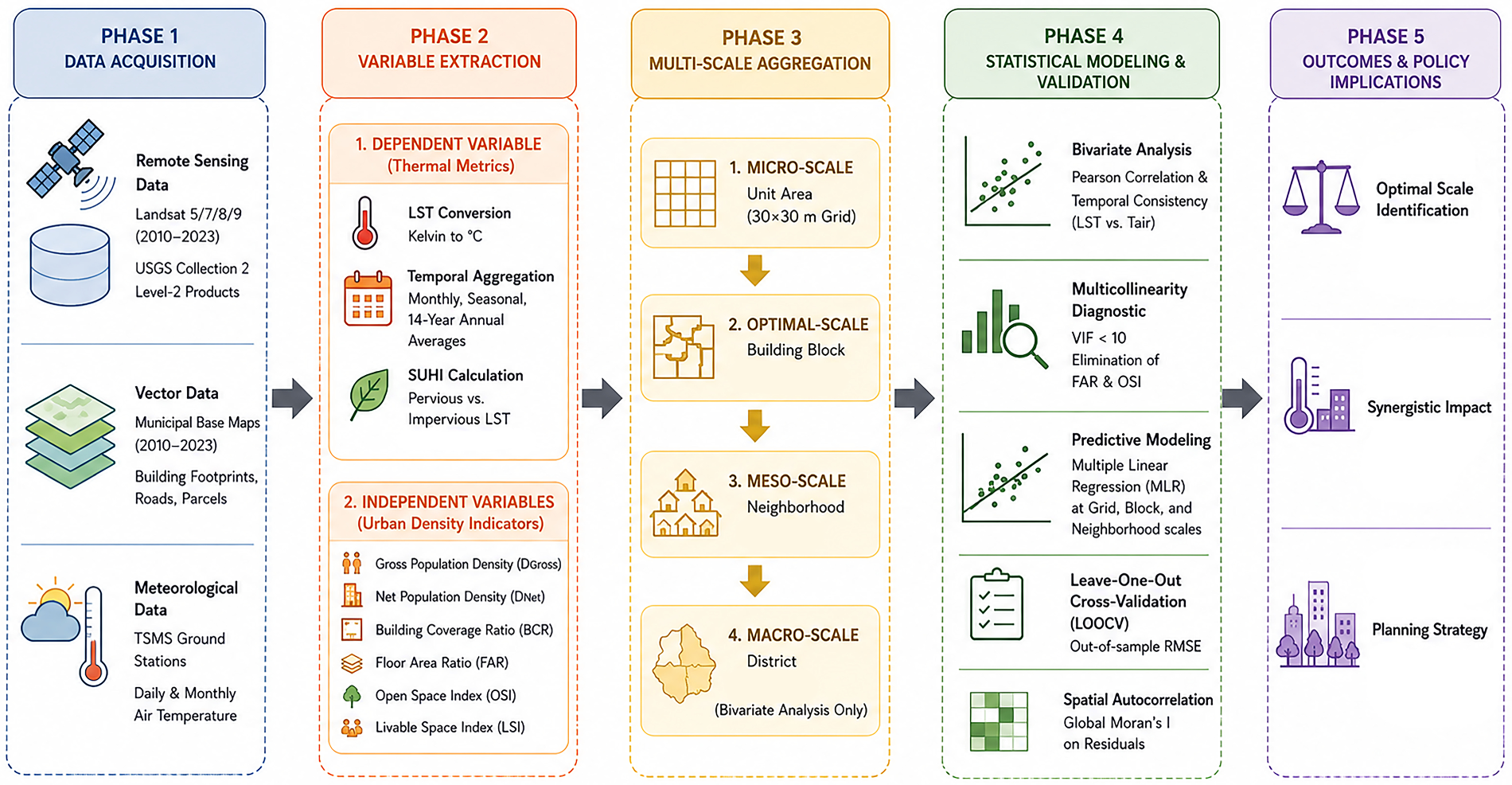
Figure 1: Workflow of this study.
The study area is located in the northwestern part of Türkiye, specifically focusing on the urban core and adjacent areas of the Çanakkale Central District (situated between 26°20′08″–26°27′07″ E longitudes and 40°01′48″–40°10′54″ N latitudes (Fig. 2). At the neighborhood scale, the analysis encompasses 12 units: seven neighborhoods from the Central district (a = Barbaros, b = Cevatpaşa, c = Esenler, d = Fevzipaşa, e = İsmetpaşa, f = Kemalpaşa, g = Namık Kemal), three neighborhoods from Kepez (h = Boğazkent, i = Cumhuriyet, j = Hamidiye), the largest town connected to the center, and two villages (k = Güzelyalı and l = Çınarlı) located within the adjacent area boundaries. At the district scale, the units are categorized into three groups: the Central District (1), Kepez Town (2), and Adjacent Areas (3). The first zone represents the highest population and construction density, while the second zone, formerly a rural settlement, has evolved into a medium-density area merging with the urban core due to rapid population growth. The third zone is characterized as a low-density settlement primarily consisting of secondary housing (summer residences).
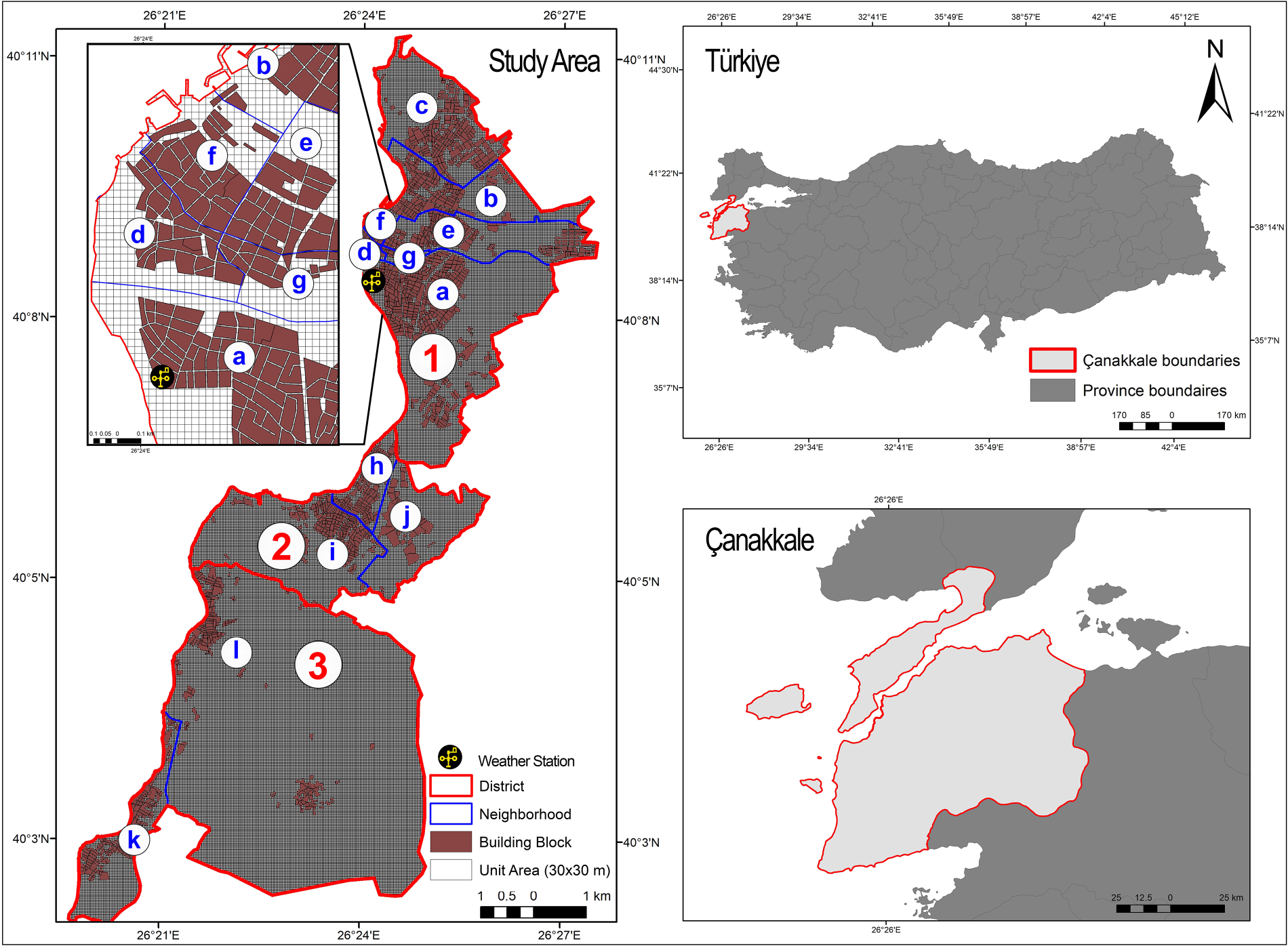
Figure 2: The study area in Çanakkale Central District, Çanakkale Province, Türkiye. The red numbers represent the districts (1: Central District, 2: Kepez Town, 3: Adjacent Areas). The blue letters inside the circles represent the study units: a = Barbaros, b = Cevatpaşa, c = Esenler, d = Fevzipaşa, e = İsmetpaşa, f = Kemalpaşa, g = Namık Kemal, h = Boğazkent, i = Cumhuriyet, j = Hamidiye, k = Güzelyalı, l = Çınarlı.
Çanakkale is located within the subtropical Mediterranean climate zone, experiencing the regional Marmara climate, which serves as a transition between Mediterranean and Black Sea climatic influences. Specifically, according to the Köppen climate classification, the study area exhibits a Csa climate type, characterized by mild winters and very hot, dry summers [42]. Based on long-term data from the Turkish State Meteorological Service (TSMS), the annual mean temperature is 15.2°C. The hottest months are July and August, with an average of 25.1°C, while the coldest month is January, averaging 6.3°C. Extreme temperatures have been recorded as high as 39.7°C in August and as low as −11.5°C in February.
The annual mean relative humidity is approximately 73%, fluctuating between 60% in summer and 80% in winter. The average annual precipitation is 624.4 mm, with the highest rainfall occurring in December (108.7 mm) and the lowest in August (10.9 mm). The average number of frost days per year is 13.4, occurring predominantly in January and February. The prevailing wind directions for the Çanakkale city center are Northeast, followed by Southwest [43]. The city’s location along the Çanakkale Strait further subjects it to significant maritime influences, which modulate local thermal dynamics.
To map the LST effects of the study area between 2010 and 2023, Landsat satellite imagery was utilized. Landsat 5, 7, 8, and 9 Collection 2 Level-2 (C2 L2) data with a 30-m spatial resolution (Path/Row: 181/032 and 182/032) were obtained from the United States Geological Survey (USGS) data portal. Due to regional climatic conditions, it is often challenging to find cloud-free and suitable images for every month within a single year. Therefore, the temporal scope of the study was expanded to a 14-year period (2010–2023) to minimize the impact of annual meteorological anomalies and to identify the long-term, stable average LST values of the area. Within this framework, a total of 142 satellite images were processed (Table S1). Monthly, seasonal, and annual average LST maps were generated by calculating the cell-based mean values for each month over the 14-year period. These Level-2 products, pre-processed by the USGS, include atmospherically and geometrically corrected surface temperature data, ensuring high radiometric consistency across the 14-year time series (Table 1).
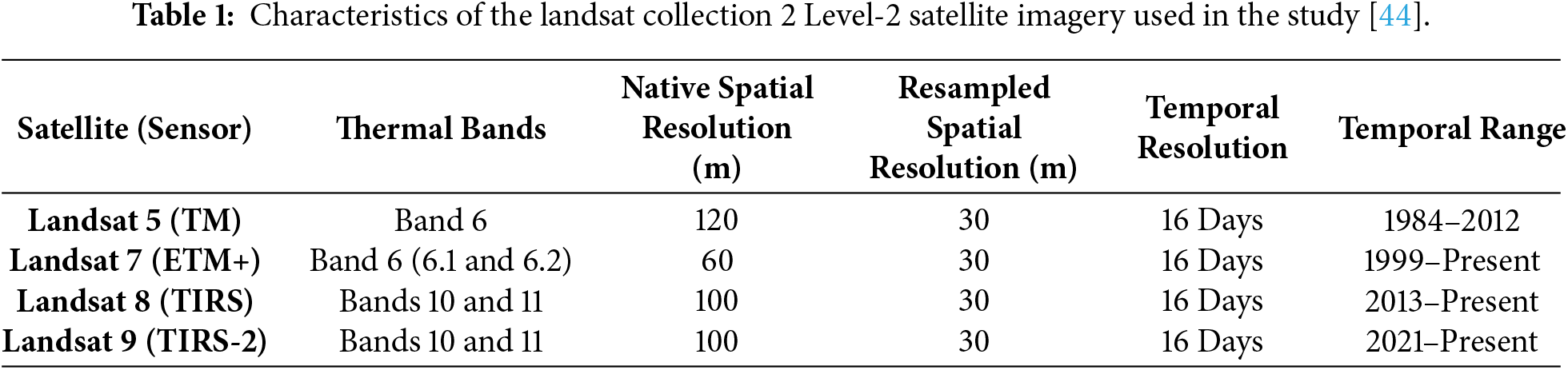
To ensure data quality, only scenes that were completely cloud-free over the study area were selected. For Landsat 7 ETM+ imagery post-2003, the Scan Line Corrector (SLC-off) data gaps were resolved using the GDAL-based ‘Fill NoData’ tool within the QGIS software environment. The missing pixels were interpolated from valid neighboring pixels using the Inverse Distance Weighting (IDW) method, followed by a smoothing filter, thereby ensuring the spatial continuity of the LST data. Since the relatively compact study area is fully encompassed by both Landsat paths 181 and 182, images from these overlapping paths were not averaged. Instead, to maximize data reliability, the single scene with the optimal visual quality, specifically the one completely free of clouds and artifacts over the study area, was selected for each given month. Furthermore, it is important to state that while the native spatial resolution of the Landsat thermal bands is coarser (120 m for TM, 60 m for ETM+, and 100 m for TIRS), all thermal datasets are resampled to 30 m by the USGS prior to distribution.
Meteorological data were utilized to evaluate the temporal consistency and seasonal cycle alignment of the satellite-derived LST data, rather than serving as a strict spatial validation. Monthly, and daily average air temperature data, synchronized with the satellite overpass dates, were obtained from the TSMS monitoring stations located within the study area (Fig. 2). These in-situ observations served as a robust reference to confirm that LST fluctuations appropriately follow regional atmospheric temperature trends. Furthermore, other microclimatic parameters, such as relative humidity, wind speed, and direction, were utilized to interpret the local drivers of UHI formation.
Urban morphology data required to calculate demographic, physical, and open space density types (BCR, FAR, Open Space Index, etc.) were produced from current base maps obtained from the Municipalities of Çanakkale and Kepez. These digital vector datasets allow for the digitization and precise calculation of building blocks, floor counts, net residential areas, and transportation/parking surfaces within a Geographic Information System (GIS) environment. Missing or outdated floor count and footprint data were updated and verified through field surveys and high-resolution satellite imagery.
To evaluate the impact of urban morphology on UHI, the 2010–2023 period was defined as a cohesive urbanization epoch, initiated by the rapid urban sprawl in 2010. The 2023 base maps and demographic data represent the mature realization of this development phase. While matching a 14-year LST average with a 2023 morphological snapshot creates a temporal lag for newly built areas (whose multi-year LST average includes pre-construction cooler years), this approach ensures that the resulting statistical relationships between density and thermal increase remain highly conservative and resistant to overestimation. This framework establishes a scientifically sound basis for evaluating the long-term cumulative thermal footprint of the recent expansion.
2.3.1 Calculation of Urban Density Indicators
To ensure reproducibility, six indicators under three main categories were quantified. The calculation formulas for each variable are as follows:
Demographic Density:
Gross Population Density (DGross): The number of people in the gross settlement area, expressed as persons/hectare (Eq. (1)). The gross area consists of the sum of the net residential area and social and technical infrastructure areas.
Net Population Density (DNet): The number of people in the net settlement area allocated solely for residential use (persons/hectare) (Eq. (2)). The net settlement area is obtained by subtracting the social and technical infrastructure areas from the gross area.
To calculate demographic density indices, neighborhood-level population data for the reference year 2023 were obtained from the Turkish Statistical Institute (TUİK) Address Based Population Registration System (ADNKS) [45]. To disaggregate the neighborhood-level population counts down to the building block and 30 m grid scales, a building based weighted dasymetric mapping approach was employed. Rather than simple areal weighting, the population was distributed proportionally based on the estimated gross floor area of the residential structures within each spatial unit, calculated by multiplying the building footprint areas by their respective number of floors. This method ensures that the 3D morphological capacity of the built environment accurately dictates the micro-scale population distribution.
Physical Density:
Building Coverage Ratio (BCR): The ratio of the building footprint to the total area of that parcel or building block (Eq. (3)).
Floor Area Ratio (FAR): The ratio of the total construction area (sum of all floors) of a building to the total area of that parcel or building block (Eq. (4)).
Open Density:
Open Space Index (OSI): In residential areas, this is obtained by dividing the unbuilt open spaces in a unit area by the total construction area within the same area (Eq. (5)). Unlike the gross BCR, this coefficient relates the open space to the construction area and, consequently, to the population living in that area. Therefore, it is considered an indicator of the quality of life.
Livable Space Index (LSI): In residential areas, this is calculated by dividing the open spaces that are unbuilt and not used by motorized vehicles (excluding roads and parking lots), thus completely available for pedestrian use, by the total construction area (Eq. (6)). As the FAR value increases, this value decreases at a certain rate depending on the number of floors of the residences.
2.3.2 Calculation of Land Surface Temperature (LST)
To determine the LST values of the study area between 2010 and 2023, pre-processed Landsat archive Collection 2 Level-2 data were utilized. Landsat Level-2 surface temperature products are generated by USGS based on the Rochester Institute of Technology (Version 1.3.0) algorithm, which effectively mitigates TIRS stray light artifacts while integrating Thermal Infrared (TIR) bands, Top of Atmosphere (TOA) reflectance, ASTER, and MERRA-2/GEOS atmospheric profile data [44].
To obtain LST in Kelvin, the official scaling formula provided by the USGS for Collection 2 Level-2 products was applied (Eq. (7)):
here, “Pixel Value” refers to Band 6 (ST_B6) for Landsat 7, and Band 10 (ST_B10) for Landsat 8 and 9. The obtained Kelvin values were converted to degrees Celsius (°C) for the final analyses (Eq. (8)):
These calculations were repeated for all months over the 14-year period between 2010 and 2023. By averaging the values on a cell basis, monthly, seasonal, and annual average LST maps were generated.
2.3.3 Spatial and Temporal Relationship Analysis
To determine at which scale the Landsat LST data with a 30-m spatial resolution are more applicable and yield more meaningful results in urban areas, the relationships between LST and urban density parameters were examined across four different spatial scales:
Unit Area (Grid) Scale: 30 m × 30 m cell size (Landsat thermal data resolution).
Building Block Scale: Average values of the cells fall within the respective building block.
Neighborhood Scale: Average values of the cells within the administrative neighborhood boundaries.
District Scale: Average values within district boundaries representing broader urban sub-regions.
For each spatial unit (e.g., a neighborhood or building block), a representative LST value was derived by calculating the arithmetic mean of the LST pixels within those boundaries. Subsequently, the density indicators (demographic, physical, and open space) were integrated with these LST values within a GIS environment.
Prior to statistical modeling, a rigorous data filtering protocol was applied to ensure the reliability of the dataset. Spatial units exhibiting GIS-related computational anomalies, specifically, where the LST was erroneously recorded as 0°C due to NoData pixels, cloud shadows, or boundary masking errors during zonal statistics, were excluded from the analysis. Importantly, unbuilt urban spaces (i.e., areas where BCR = 0) were deliberately retained in the dataset to accurately evaluate the cooling effects of open spaces and parks. This multi-scale framework allowed for a systematic comparison of thermal-morphological interactions throughout the time series (2010–2023), facilitating the identification of the scale at which urban heat dynamics are most accurately captured while minimizing micro-scale thermal noise.
Correlation and regression analyses were employed to examine the direction and magnitude of the relationship between urban density parameters and LST. The Pearson correlation coefficient (r) was utilized to determine the linear relationship between variables, while probability (p) values were used to test the statistical significance of the findings [46].
To account for the complex and multi-dimensional structure of urban morphology, MLR models were developed. As a methodological necessity, the district scale was excluded from multivariate modeling due to an insufficient sample size (n = 3). Therefore, the regression analyses were conducted exclusively across the remaining three spatial scales (unit area, building block, and neighborhood). A critical step in the modeling process involved addressing multicollinearity, as urban density parameters, such as BCR and FAR, often exhibit high internal correlation. To ensure model reliability, Variance Inflation Factor (VIF) values were calculated for all independent variables. Following established statistical protocols, variables exceeding a VIF threshold of 10 were systematically excluded from the models to prevent coefficient inflation and ensure statistical stability [47].
In addition to the explanatory power indicated by the Adjusted R2
Traditional MLR assumes that the residuals (estimation errors) are independent and randomly distributed. However, urban thermal environments often exhibit spatial dependence, where the LST of a specific unit is influenced by its adjacent neighbors (heat spillovers). To assess this spatial dependence and validate the OLS assumptions, a Global Moran’s I diagnostic was applied to the model residuals. Global Moran’s I is a robust statistic that measures the overall spatial autocorrelation across the study area. The index (I) is calculated using Eq. (9):
where n is the total number of spatial units (building blocks), xi and xj represent the regression residual values for spatial units i and j,
In this study, spatial relationships were conceptualized an Inverse Distance method based on Euclidean distance, and row standardization was applied to mitigate bias from unevenly distributed features. To determine the statistical significance of the observed spatial autocorrelation, the z-score is calculated using Eq. (10):
where E[I] is the expected value of Moran’s I under the null hypothesis of no spatial autocorrelation, and V[I] represents its variance. A statistically significant positive z-score (z > 1.96, p < 0.05) indicates spatial clustering of the estimation errors, thereby highlighting the necessity of acknowledging spatial dependence in micro-scale thermal analysis.
All spatial data processing and GIS analyses were conducted using QGIS Desktop 3.30.2 and ArcMap 10.5. Statistical analyses, including multicollinearity diagnostics and MLR were performed using Python within the Jupyter Lab environment.
In this study, spatial, morphological, and temporal relationships between urban density parameters and LST were analyzed using a 14-year climatological dataset (2010–2023). The findings are presented in four subsections: the validation of LST data against meteorological parameters, bivariate correlations across spatial scales, a multi-scale regression modeling including temporal dynamics, and monthly and seasonal dynamics of LST.
3.1 Temporal Consistency and Seasonal Cycle Check with Meteorological Parameters
To evaluate the temporal reliability and seasonal consistency of the satellite-derived LST data, a comparative analysis was conducted using ground-based meteorological observations from the 2010–2023 period. The relationship between the monthly mean air temperature and the monthly mean LST showed a very strong positive correlation (r = 0.96) (Fig. 3). While this high correlation primarily reflects a shared seasonal cycle rather than a strict spatial validation, it confirms that LST fluctuations robustly follow regional atmospheric temperature trends.
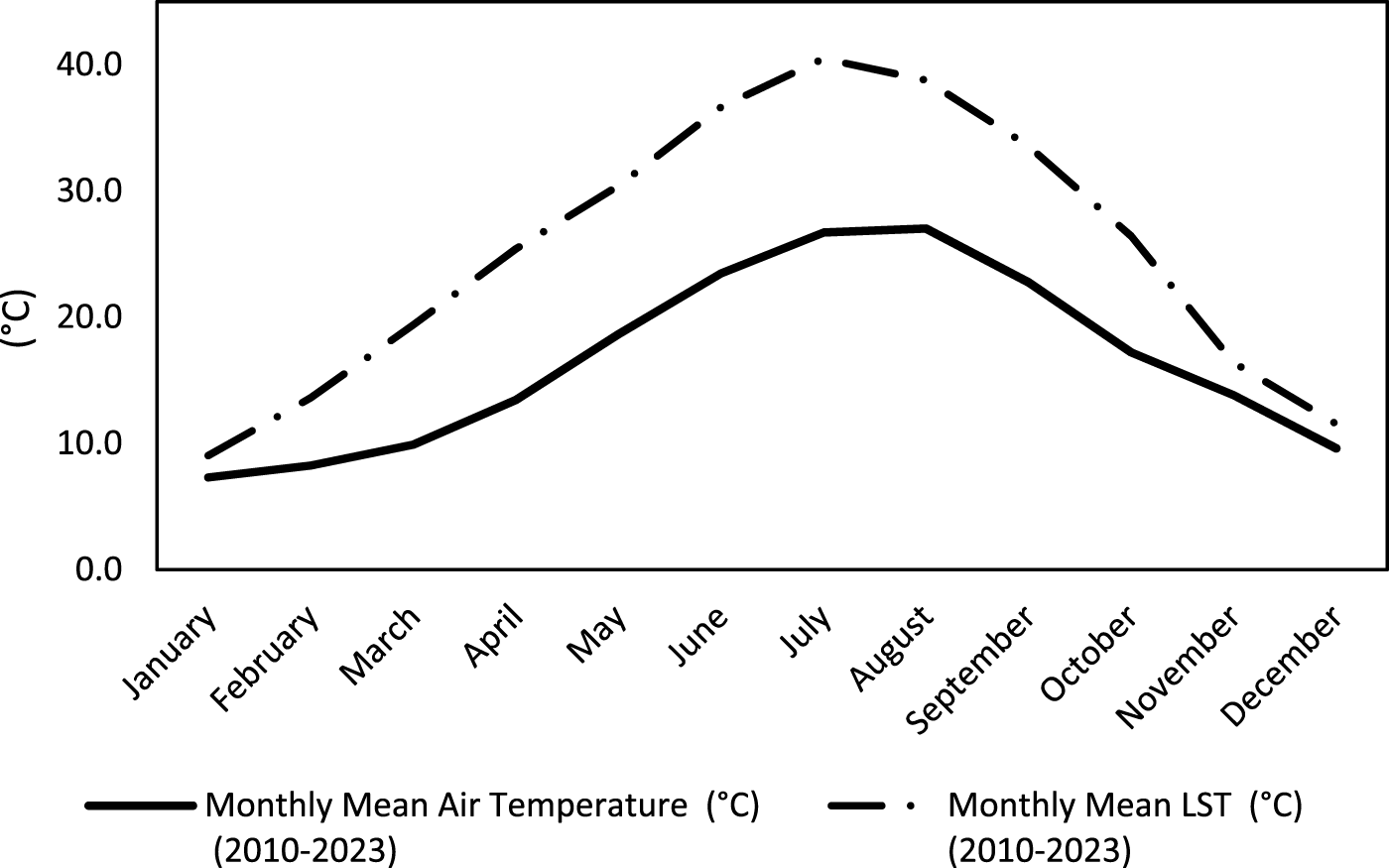
Figure 3: The relationship between air temperature and LST.
Furthermore, a strong positive correlation (r = 0.83) was identified between air temperature and the standard deviation of LST (Fig. 4). This relationship suggests that as air temperatures rise, the thermal heterogeneity of the urban surface increases, primarily due to the differential heat-retention and re-radiation capacities of impervious surfaces. This phenomenon explains the peak in thermal variance during the summer months, when the contrast between heat-absorbing built-up areas and natural surfaces is most pronounced.
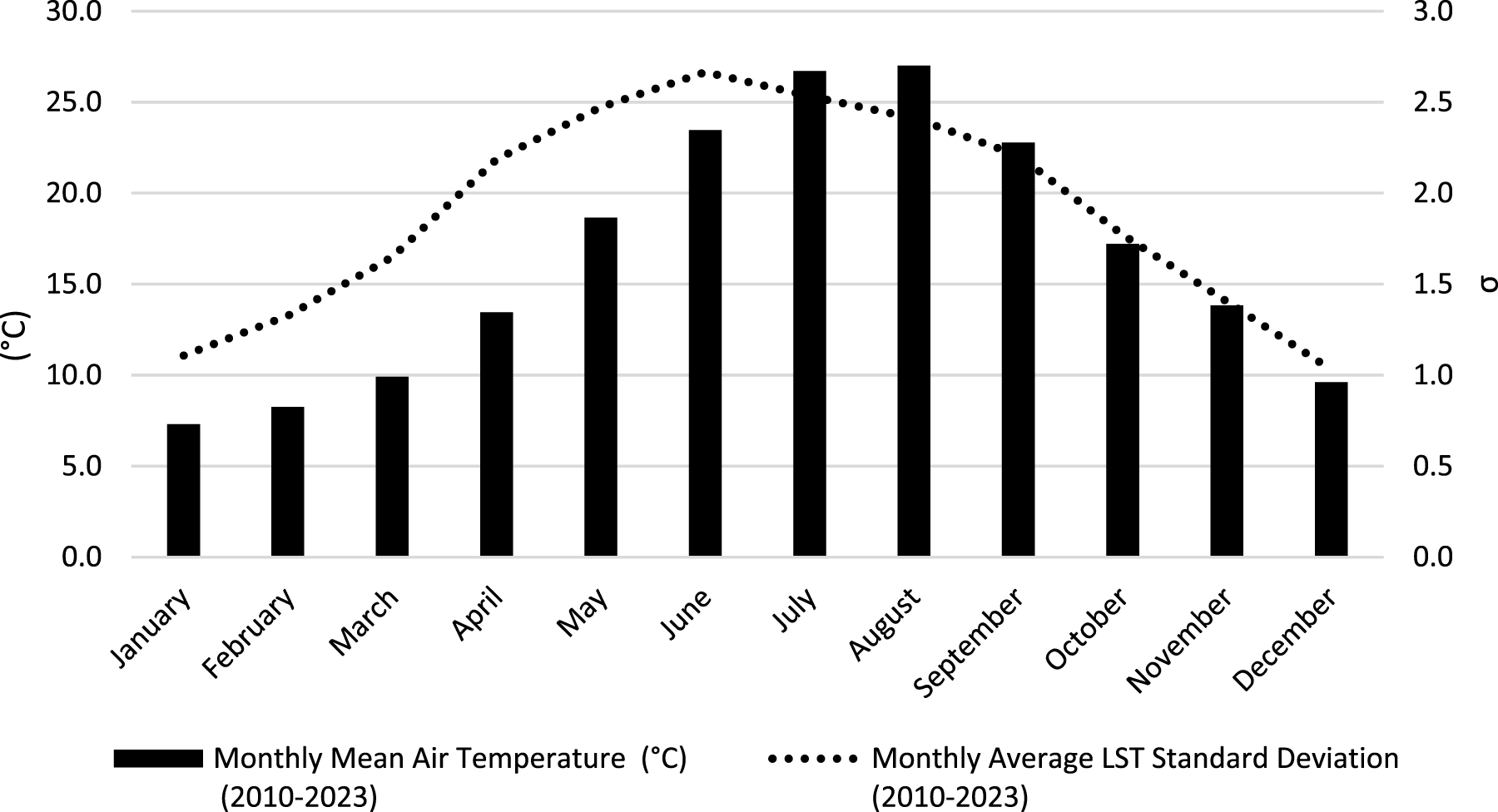
Figure 4: Standard deviation of monthly average air temperature and LST values.
A direct comparison between the LST values extracted from specific satellite overpass dates and the corresponding daily mean air temperatures yielded a high positive correlation (r = 0.94) (Fig. 5). As illustrated in the regression analysis (Fig. 5), the model exhibits a slope of 1.38 and an intercept of 2.43 (R2 = 0.90, RMSE = 10.15°C, Bias = 9.17°C). The slope greater than 1 indicates systematic amplification is a physically expected characteristic for daytime observations over impervious urban surfaces, where sensible heat fluxes dominate and physical surfaces heat up significantly faster than the overlying air. This effect is further pronounced because instantaneous daytime LST captures near-maximum solar heating, whereas the daily mean air temperature includes cooler nighttime values. This structural difference highlights the robust heat exchange mechanism between the land surface and the lower atmosphere, explicitly demonstrating the vulnerability of urban morphology to thermal stress.
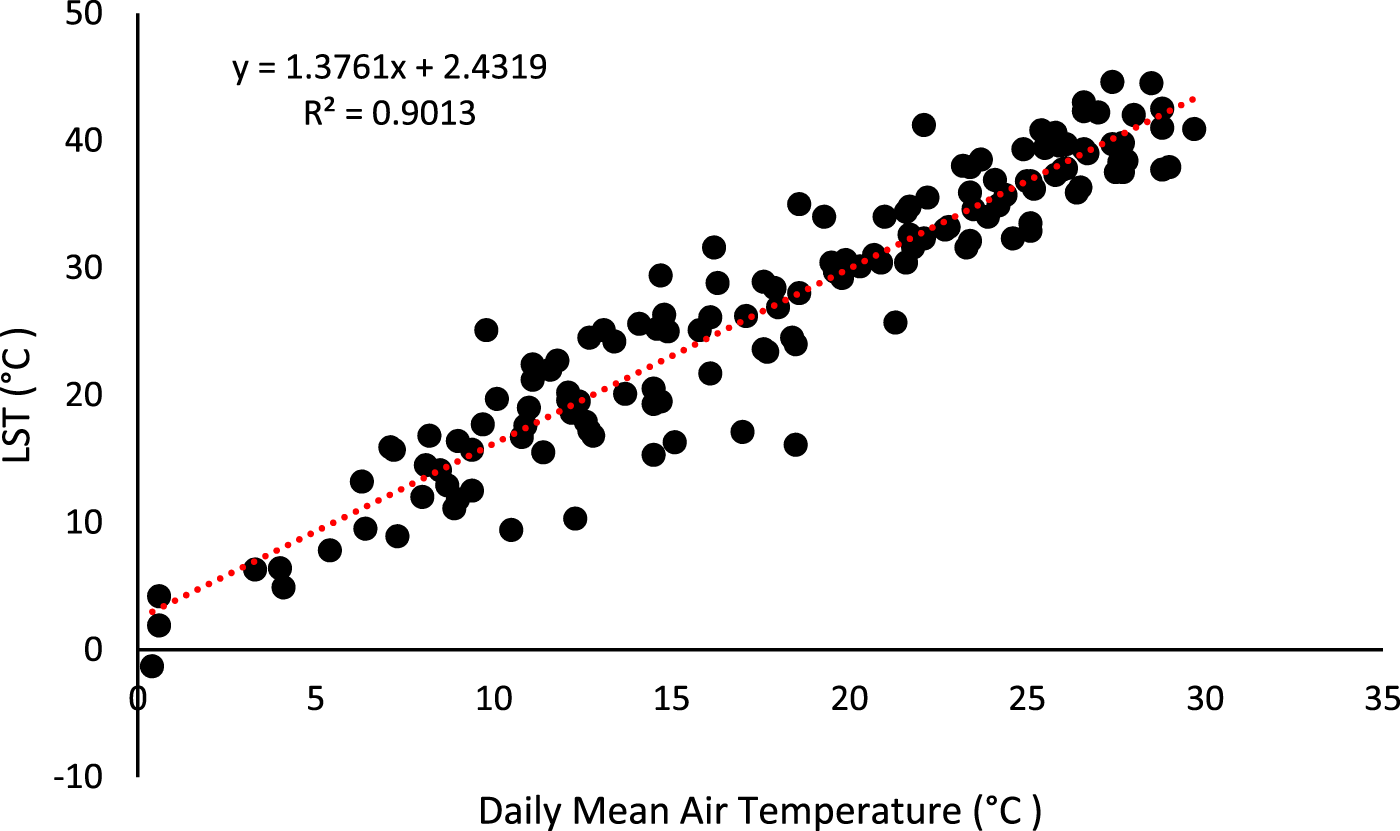
Figure 5: The relationship between the dates satellite images were captured and the corresponding daily air temperature data.
3.2 Bivariate Correlations across Spatial Scales
Pearson correlation analyses were conducted to evaluate the initial linear interactions between the six urban density parameters and LST across four spatial scales: Unit Area (30 m Grid), Building Block, Neighborhood, and District.
The analysis revealed that the correlation strengths are highly sensitive to spatial scale (Fig. 6). At the micro-scales (Unit Area and Building Block), the annual correlation coefficient remained weak to moderate (|r| ≤ 0.32). A significant increase was observed at the neighborhood scale, where DGross exhibited the strongest positive correlation (r = 0.73, p < 0.001), while the OSI and LSI demonstrated strong negative correlations (r = −0.57). At the macro (District) scale, the bivariate correlations for all density parameters reached extreme values (|r| > 0.95). However, from a critical methodological perspective, this scale is characterized by an extremely small sample size (n = 3). In spatial statistics, reporting such high correlations at heavily aggregated levels serves as a classic demonstration of the Modifiable Areal Unit Problem (MAUP) and aggregation bias. As spatial data is grouped into fewer, larger administrative boundaries, micro-scale variance is artificially filtered out, systematically inflating the correlation coefficients. Therefore, these district-level values are presented here not as stable predictive metrics, but rather as an empirical warning for urban climate researchers regarding how scale inflation masks actual ground-level thermal dynamics. To establish true statistical validity at this administrative resolution, a substantially larger institutional sample size of distinct districts would be required.
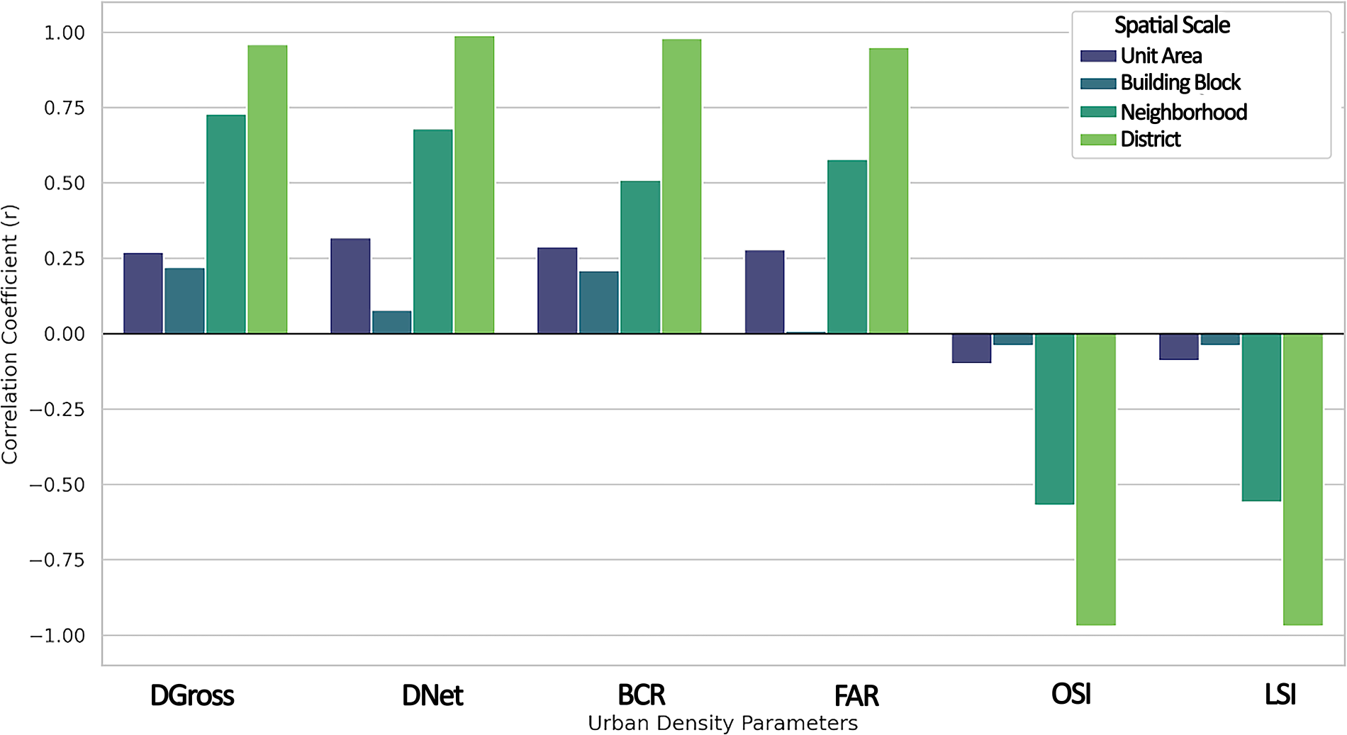
Figure 6: Annual correlation between urban density and LST across different scales.
3.3 Multicollinearity Diagnostic and Multiple Linear Regression (MLR)
To identify the primary morphological drivers of LST, MLR models were constructed. As a methodological necessity, the district scale was excluded from multivariate modeling due to an insufficient sample size (n = 3 for the analyzed district). The regression analyses were thereby conducted on the Unit Area, Building Block, and Neighborhood scales.
Prior to modeling, VIF diagnostics were performed to address multicollinearity among the density parameters. The results indicated that the OSI and FAR consistently exceeded the accepted threshold of VIF > 10 across the analyzed scales. Consequently, these variables were removed using backward elimination. Crucially, to allow for a direct comparison of predictors with vastly different native units (e.g., BCR as a 0–1 ratio vs. demographic density as person/ha), all remaining independent variables were standardized prior to regression. The final MLR models were established using the remaining independent variables: DGross, DNet, BCR, and LSI.
The explanatory power of the resulting MLR models varied significantly by scale, demonstrating a clear scale-dependent progression. At the Unit Area scale, the model yielded a very low Adjusted R2 of 0.032. In contrast, the aggregated scales demonstrated substantially higher and nearly identical explanatory power: the Adjusted R2 was 0.314 for the Building Block scale and 0.447 for the Neighborhood scale. However, evaluating models solely on in-sample fit metrics like Adjusted R2 can be misleading, particularly for aggregated scales with smaller sample sizes. To rigorously test predictive reliability and address potential overfitting, LOOCV was performed. The results revealed a critical methodological insight while the Neighborhood scale exhibited the lowest in-sample RMSE (0.54°C), its out-of-sample LOOCV RMSE drastically spiked to 13.53°C. This severe performance collapse confirms that the high explanatory power at the Neighborhood level (n = 12) is largely an artifact of overfitting. In stark contrast, the Building Block scale (n = 1396) maintained robust predictive stability, yielding nearly identical in-sample (0.92°C) and out-of-sample (0.93°C) error metrics. This cross-validation mathematically confirms the Building Block as the optimal spatial resolution for urban design interventions.
Fig. 7 illustrates the high in-sample predictive precision across the three spatial scales. While the Neighborhood scale shows a good fit in Fig. 7, it is essential to interpret this in conjunction with the LOOCV cross-validation metrics presented in Table 2. This comparison reveals that the exceptional fit at the Neighborhood scale is a statistical artifact of overfitting (n = 12), whereas the Building Block scale maintains robust predictive stability on unseen data.
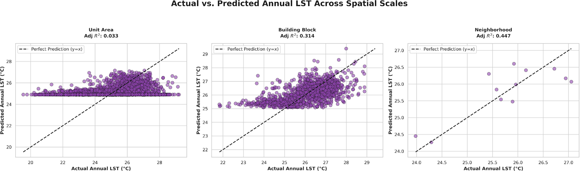
Figure 7: In-sample predictive performance of the MLR models across three spatial scales (predicted vs. actual LST). The extremely tight fit observed at the neighborhood scale (right panel) visually demonstrates the high in-sample R2, which is subsequently identified as a statistical artifact of overfitting due to the small sample size (n = 12).
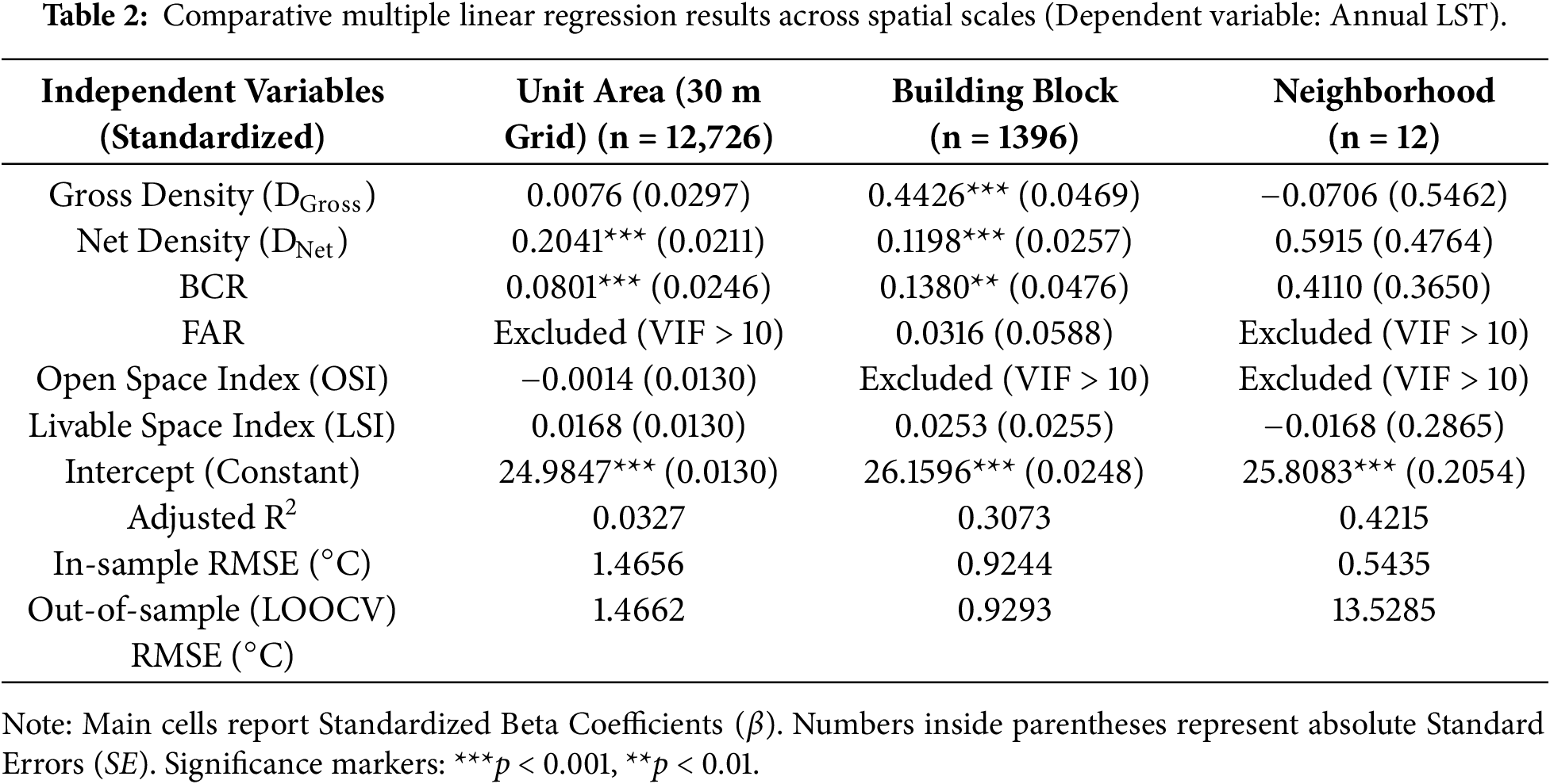
Analysis of the standardized beta coefficients (β) revealed that DGross and BCR were the dominant and most significant positive predictors of LST at the Building Block scale (Table 2). Specifically, both variables showed strong independent effects, with DGross (β = 0.443, p < 0.001) and BCR (β = 0.138, p = 0.003) standing out as a critical driver of urban heat. By utilizing standardized coefficients, this statistical prominence is established independent of the variables’ original measurement scales.
However, while the overall explanatory power of the model appeared to increase at the Neighborhood scale, the statistical significance of individual predictors completely vanished (p > 0.05). This loss of predictor significance is likely due to the combination of thermal homogenization across large boundaries and the extremely small sample size (n = 12). Conversely, at the Unit Area (30 m) scale, only DNet and BCR emerged as statistically significant positive predictors, though the model’s overall capacity to explain temperature variations remained negligible.
To evaluate the spatial dependence of the urban thermal environment and validate the assumptions of the Ordinary Least Squares (OLS) framework, a Global Moran’s I diagnostic was performed on the model residual at the optimal Building Block scale. Table 3 presents the spatial autocorrelation statistics for the residual of each density metric. The analysis revealed a highly significant positive spatial autocorrelation (clustered pattern) for the residuals of structural density metrics, specifically the BCR (I = 0.596, z = 122.56, p < 0.001) and FAR (I = 0.534, z = 109.79, p < 0.001). This strong clustering indicates that the thermal behavior of physical urban forms is not completely isolated; rather, the heat trapped by contiguous impervious surfaces and building volumes spills over into adjacent spatial units. Consequently, estimation errors in these structural models are spatially agglomerated, demonstrating the inherent thermal continuity of the built environment and suggesting that future micro-scale studies could benefit from spatial regression techniques (e.g., Spatial Error or Spatial Lag Models) to yield completely unbiased coefficient estimates.
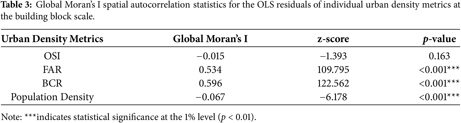
Conversely, the spatial patterns of residuals for demographic and open space metrics exhibited fundamentally different thermal behaviors. The residuals for the OSI demonstrated a completely random spatial distribution (I = −0.015, z = −1.39, p = 0.163), indicating an absence of spatial autocorrelation. This confirms that the localized cooling effect of unbuilt spaces is strictly confined to their immediate vicinity without significant spatial spillover, making the standard OLS framework perfectly sufficient for capturing its impact without spatial bias. In particular, the residuals for Population Density displayed a slight but statistically significant dispersed pattern (I = −0.067, z = −6.17, p < 0.001). This negative autocorrelation reflects the highly heterogeneous and fragmented distribution of demographic density, and its associated anthropogenic heat emissions, within the urban fabric. Together, these diagnostics highlight that while physical building coverage induces contiguous thermal zones, demographic and open space impacts operate in a highly localized and diverse manner across the micro-climate.
3.4 Monthly and Seasonal Dynamics
Temporal variations in the density-LST relationship were analyzed using 14-year monthly and seasonal averages to account for intra-annual microclimatic shifts. The spatiotemporal analysis of LST across Çanakkale reveals a consistent thermal gradient between the urban core and its periphery (Figs. 8–10). The annual mean LST (Fig. 8) highlights permanent thermal hotspots in high-density built-up areas, where temperatures are significantly higher than in the surrounding vegetated zones.
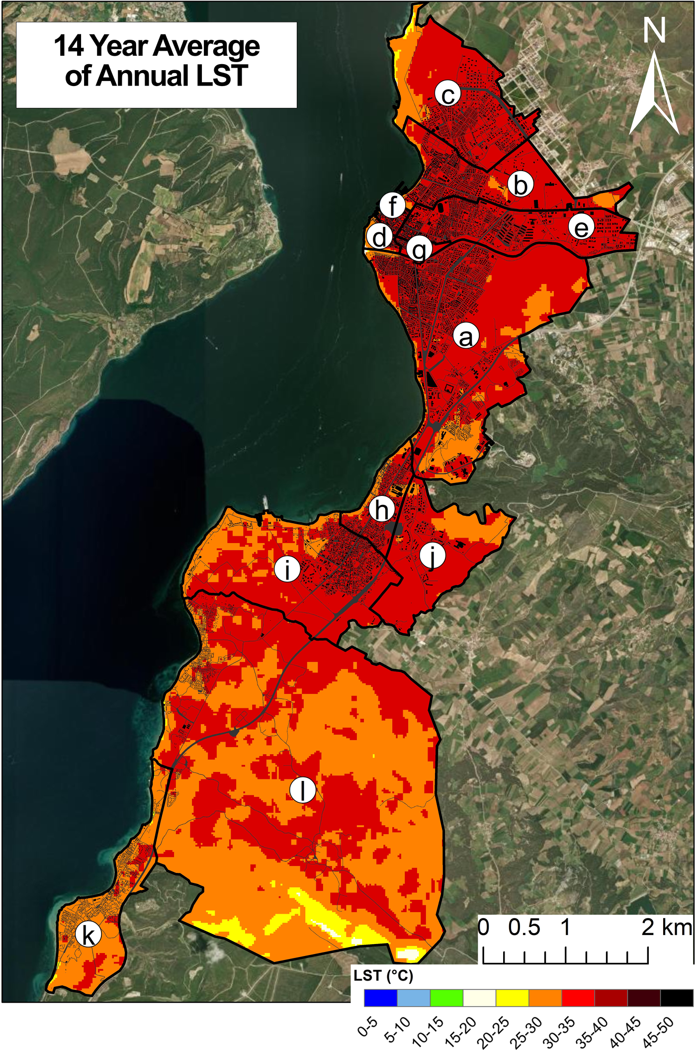
Figure 8: Annual mean LST (2010–2023). Letter codes represent individual neighborhoods (a = Barbaros, b = Cevatpaşa, c = Esenler, d = Fevzipaşa, e = İsmetpaşa, f = Kemalpaşa, g = Namık Kemal, h = Boğazkent, i = Cumhuriyet, j = Hamidiye, k = Güzelyalı, l = Çınarlı.), while bold black outlines indicate district boundaries. Building footprints and road networks are overlaid in black to illustrate the relationship between physical density and thermal hotspots.
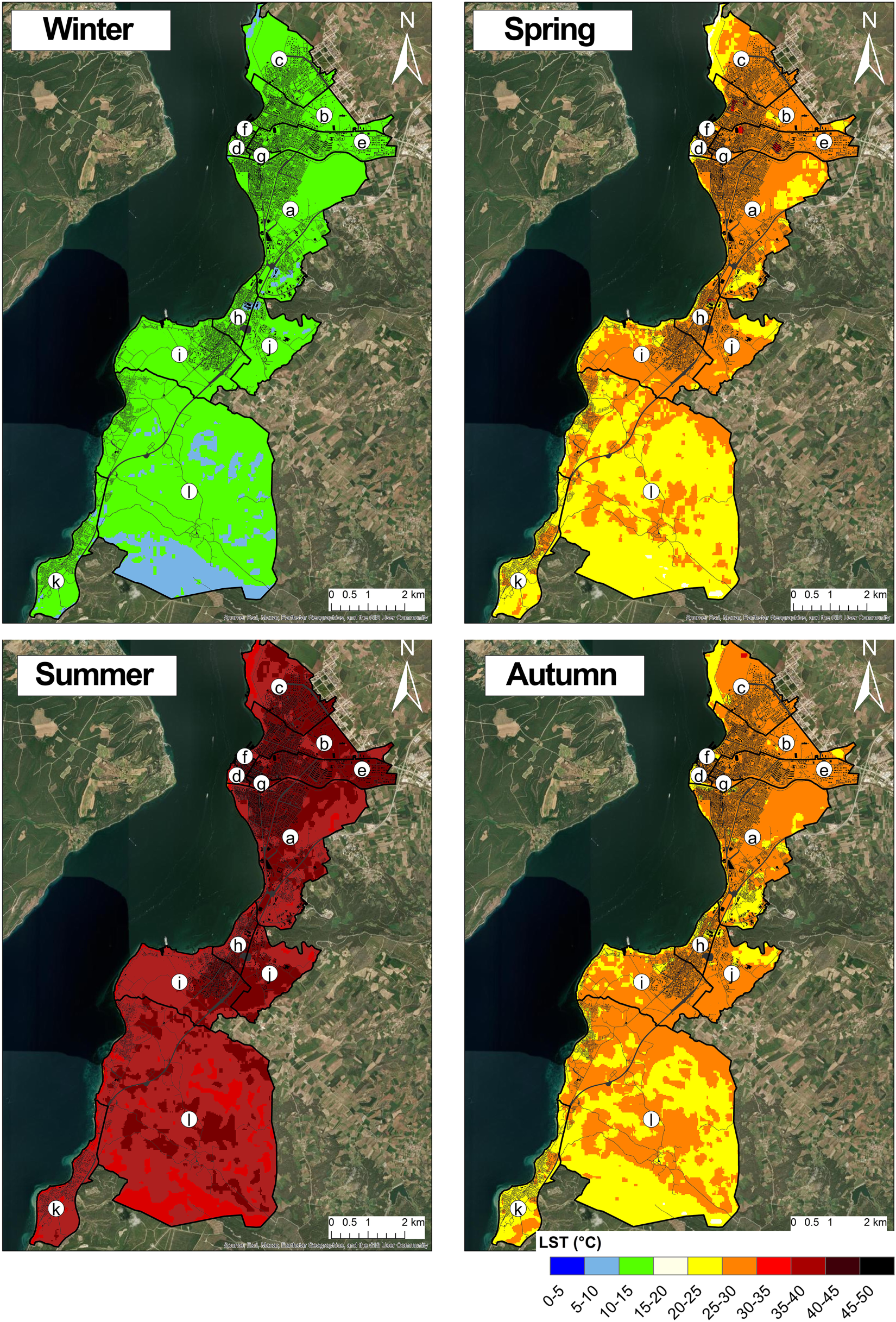
Figure 9: Seasonal LST variations. Letter codes represent individual neighborhoods (a = Barbaros, b = Cevatpaşa, c = Esenler, d = Fevzipaşa, e = İsmetpaşa, f = Kemalpaşa, g = Namık Kemal, h = Boğazkent, i = Cumhuriyet, j = Hamidiye, k = Güzelyalı, l = Çınarlı.), while bold black outlines indicate district boundaries. Building footprints and road networks are overlaid in black to illustrate the relationship between physical density and thermal hotspots.
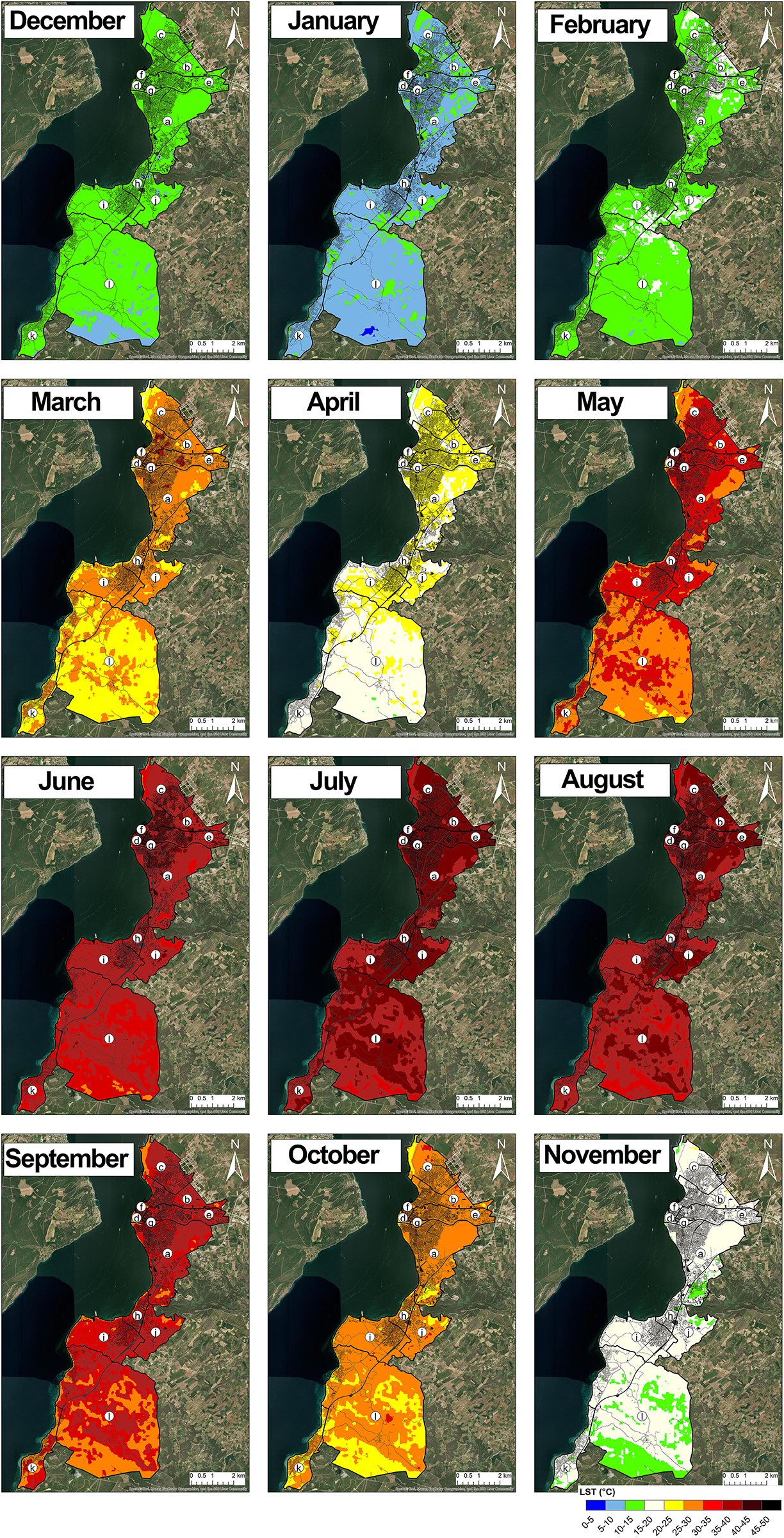
Figure 10: Monthly LST progression. Letter codes represent individual neighborhoods (a = Barbaros, b = Cevatpaşa, c = Esenler, d = Fevzipaşa, e = İsmetpaşa, f = Kemalpaşa, g = Namık Kemal, h = Boğazkent, i = Cumhuriyet, j = Hamidiye, k = Güzelyalı, l = Çınarlı.), while bold black outlines indicate district boundaries. Building footprints and road networks are overlaid in black to illustrate the relationship between physical density and thermal hotspots.
Seasonal mappings (Fig. 9) demonstrate that the spatial extent of high LST values expands during Spring and Summer, reaching its maximum spatial extent and intensity. In contrast, Winter maps show a more uniform thermal surface with minimized temperature contrasts. Monthly distributions (Fig. 10) track the transition of these patterns, showing a steady intensification of heat clusters from early spring through mid-summer. Notably, spatial homogenization of the thermal surface is observed in September, where the distinct urban-rural temperature boundaries temporarily weaken before transitioning into the winter equilibrium.
Across all valid scales, the strongest positive correlations between the urban density parameters and LST were consistently recorded during the spring months, peaking specifically in April and May (e.g., r = 0.70–0.75 on the Neighborhood scale). During the summer peak (July and August), when absolute LST reaches its maximum, the correlation strengths exhibited a slight decrease compared to the spring peak.
A distinct statistical anomaly was observed during the autumnal transition in September. To illustrate the magnitude spatial consistency of this phenomenon, a multi-scale monthly correlation matrix was generated. As visualized in the heatmap (Fig. 11), September marks an abrupt microclimatic homogenization, causing a simultaneous statistical collapse across all structural parameters, especially at district scale.
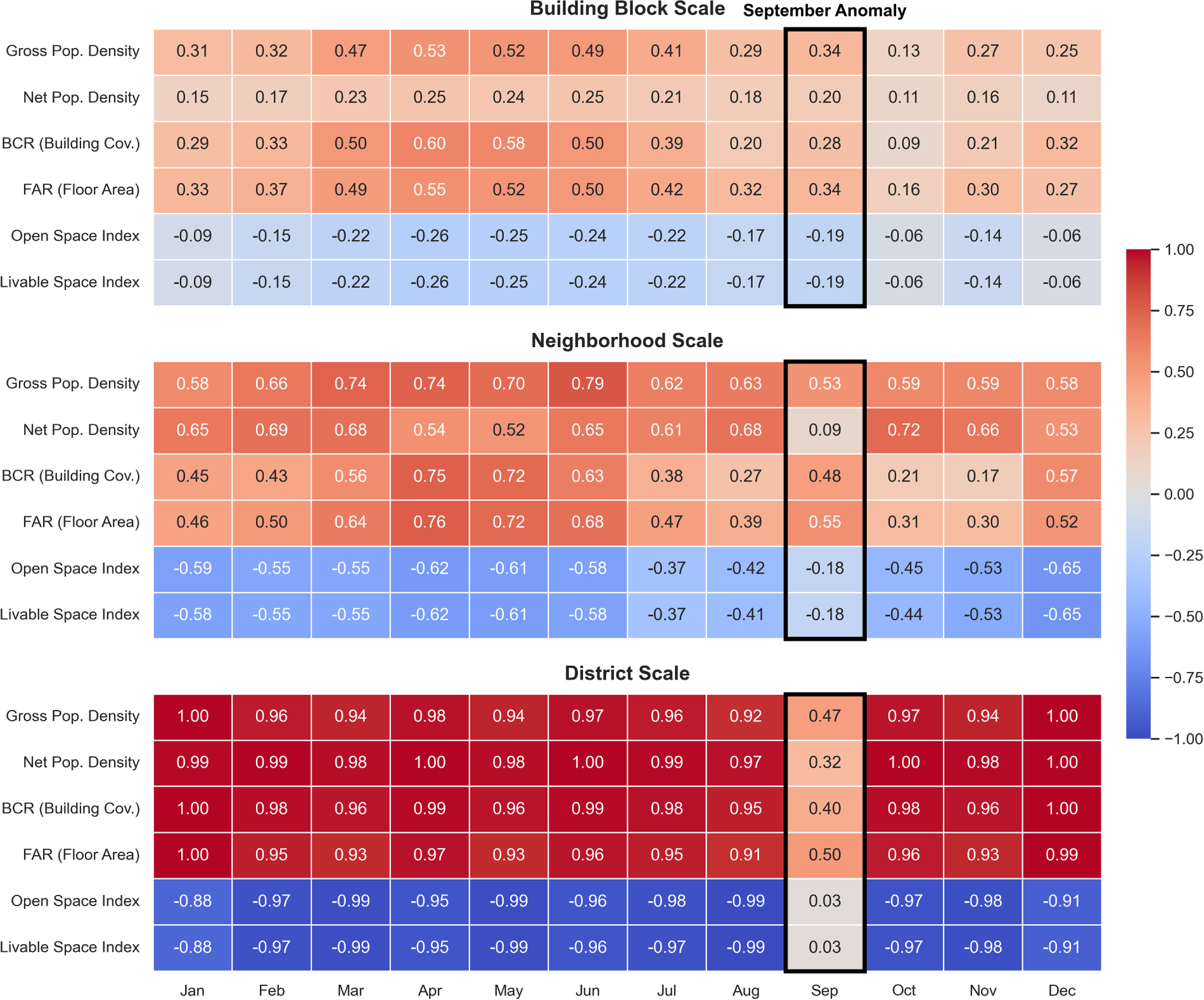
Figure 11: Multi-scale heatmap of Pearson correlation coefficients between urban density parameters and monthly LST values (January–December).
The heatmap explicitly confirms that this loss of explanatory power is not an isolated event at the macro (i.e., district) level, but a systemic disruption that occurs consistently down to the Building Block and Neighborhood scales, where r values drop sharply to near-zero. Following this September anomaly, correlation strength recovered gradually throughout the autumn and winter months, re-establishing a strong linear relationship as the region entered its winter climatological regime.
The research results demonstrate that the LST exhibits a heterogeneous distribution across different scales, primarily driven by demographic and physical density. The systematic identification of higher LST values in areas with intensive building density and impervious surface ratios aligns with similar findings in the literature [39,48–50]. However, the MLR models used in this study reveal that the BCR parameter has a significant combined effect on LST in conjunction with demographic density. These findings are consistent with studies emphasizing the absolute dominance of horizontal morphological expansion over the urban thermal environment [51].
Seasonal analyses confirm that the response of LST to physical indicators varies according to the climatic context [52]. While the high heat accumulation capacity of impervious surfaces intensifies this difference during summer and autumn [53,54], the “September Anomaly” observed in this study is hypothesized to be linked to the thermal lag phenomenon specific to coastal cities. Recent SHAP-based attributions demonstrate that water bodies can exhibit a “sign reversal” effect, transforming into potential heat accumulation sources during specific seasonal contexts due to their high specific heat capacity [55]. The delayed cooling of seawater compared to land, combined with the temporal decoupling between anthropogenic heat sources and climatic data, is thought to contribute to the weakening of correlations in September [56,57].
From a methodological perspective, the dramatic increase in explanatory power (R2) when transitioning from the micro-scale (30 m Grid) to the Building Block and Neighborhood scales is linked to the thermal blurring effect in Landsat data. At the micro-scale, the model yielded an extremely low R2 of 0.033, as the resampling of 100 m thermal data to 30 m creates radiometric noise between structural and thermal data at the micro-level. The mitigation of this noise through aggregation at the building block (
While various studies suggest different optimal scales such as 180 or 600 m or recently identified 250–300 m thresholds [40,41,59], this study demonstrates that the building block scale provides the highest statistical reliability and practical resolution for urban design interventions specifically within the context of Çanakkale. Although the Neighborhood scale initially appears to yield higher explanatory power, its susceptibility to spatial overfitting leaves the Building Block as the ultimate reliable spatial unit that balances statistical accuracy with the preservation of practical morphological details. Furthermore, the identification of the building block as the optimal scale is strongly supported by recent literature. As Reference [60] emphasizes, employing block units structured by road networks rather than arbitrary grids avoids the bisection of building footprints, ensures morphological homogeneity, and more accurately reflects human activities, thereby effectively filtering out micro-scale radiometric noise.
The analysis confirms that BCR and DGross act synergistically as the primary morphological indicators associated with urban temperature, especially at the building block scale. While standardized coefficients highlight their relative statistical importance, understanding the physical equivalent of these metrics is critical for urban planning decisions. According to the unstandardized baseline MLR estimates, holding all other parameters constant, every %10 increase in BCR (0.10 unit**, derived from the unstandardized coefficient of 0.813**) correlates with an approximate rise of 0.08°C in local annual temperature. As deciphered in the spatial design simulation (Fig. 12), transitioning from a BCR of 0.10 (Detached Fabric) to 0.90 (dense Attached Fabric) does not merely increase concrete mass; it eliminates the void volume that allows the block to breathe. Indeed, recent literature strongly supports the idea that urban green space ecosystems and open voids play a fundamental role in mitigating urban heat islands [61].
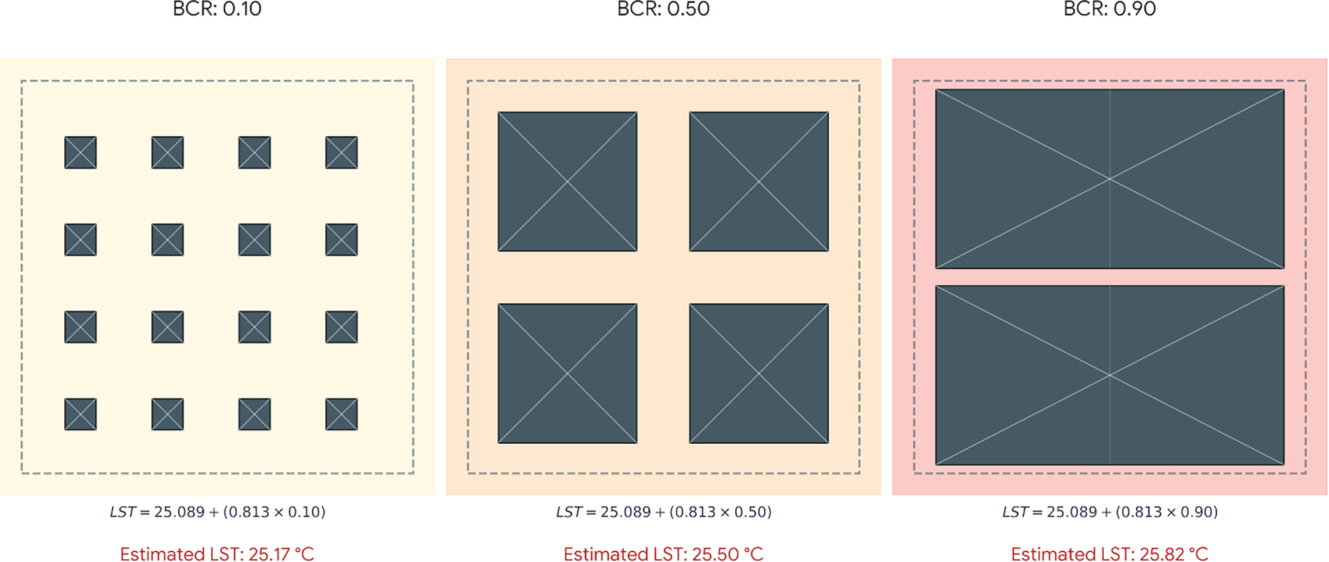
Figure 12: Comparative simulation of the relationship between BCR and estimated LST at the building block scale. The visual demonstrates the transition from detached (low BCR) to dense attached (high BCR) urban fabrics, where each 0.10 unit increase in BCR is linked to a statistically significant thermal rise based on the MLR coefficient (0.813).
Furthermore, it is crucial to accurately interpret the impact of demographic density alongside the physical footprint. While BCR controls passive solar heating, DGross reflects the active, anthropogenic heat introduced into the micro-climate. According to the unstandardized baseline building block model, the unstandardized coefficient for DGross is 0.0021. In practical urban planning terms, this means that for every 100 additional people settling within a 1-hectare building block (100 person/ha), the local annual mean temperature rises by approximately 0.21°C. This temperature increase is associated with the concentrated anthropogenic heat fluxes resulting from population density, such as increased vehicular traffic, the operation of air conditioning units, and higher daily energy consumption, rather than human body heat itself. This synergistic effect of dense built environments and high population concentrations drastically amplifies localized cooling demand, a critical mismatch recently emphasized by References [62,63], who demonstrated that core urban areas with high demographic exposure face the most severe and urgent heat risks.
The negative correlation found between LST, and the LSI further supports the cooling effect of open spaces and void management [64]. Furthermore, evidence suggests that road width can increase wind speed by 90%, whilst open spaces can increase it by 50% [65]. It demonstrates that the contraction of these breathing spaces renders urban areas more climatically vulnerable. Therefore, sustainable urban design should prioritize the solid-void relationship on the ground rather than just aggregate density.
The significant positive spatial autocorrelation (Moran’s I = 0.596) observed in the MLR residuals at the building block scale highlights the inherent spatial dependence of urban micro-climates. This clustering indicates that the thermal behavior of a building block is not entirely isolated but interacts continuously with adjacent blocks, leading to localized heat spillover effects. This strong spatial dependence is consistent with recent findings demonstrating that localized urban environmental performance is heavily dictated not only by on-site conditions but also by the surrounding urban fabric [66] While the primary objective of this study was to mathematically compare relative explanatory power across four different spatial scales using a standardized baseline MLR framework, this spatial dependence cannot be ignored in predictive modeling. Therefore, future studies are highly encouraged to adopt Spatial Error Models (SEM) or Spatial Lag Models (SLM) to account for thermal spillovers and further refine local coefficient estimates. As recently demonstrated by references [60,61], moving beyond traditional OLS to advanced spatial econometric models is essential for accurately capturing the spatial heterogeneity and thermal interactions of adjacent urban units.
Despite the strong evidence presented, this research has certain limitations. First, LST is satellite-derived data and may differ from the ambient air temperature directly felt by humans. Second, three-dimensional data such as building heights (H) and 3D urban canyon geometry (H/W ratio) could not be fully integrated into the analyses due to data constraints; however, the shading effect of buildings remains a secondary control mechanism. Finally, the factors supporting the September anomaly are presented as statistical inferences; validating these theories with direct energy consumption data and coastal wind stations in future studies will further strengthen the framework.
This study deconstructs the multi-scale relationship between urban morphology and LST in the coastal city of Çanakkale over a 14-year period. The findings reveal a significant scale dependency, identifying the Building Block scale as the optimal spatial resolution for urban design interventions. While the Neighborhood scale yields the highest explanatory power (
A critical discovery of this research is the synergistic impact of physical and demographic densities on the urban micro-climate. Based on standardized Beta coefficients, DGross (β = 0.4426) and the BCR (β = 0.1380) act jointly as the primary indicators associated with localized thermal increases. While every 10% increase in BCR is associated with an approximately 0.08°C rise in surface temperature, the standardized metrics highlight that horizontal physical coverage, and anthropogenic demographic concentration must be managed simultaneously. Furthermore, the identified September anomaly proves that coastal urban climates are subject to seasonal shifts and maritime thermal lag, necessitating month-specific mitigation strategies. In coastal cities, this seasonal extension of thermal stress suggests that climate adaptation measures, such as urban cooling interventions and energy management policies, should not be limited to peak summer months but must extend into late autumn to address the prolonged heat.
From a policy perspective, these results suggest that climate-sensitive urban planning should prioritize breathing design models that preserve open-space voids and regulate ground-level coverage to prevent heat trapping. The structural stability of the Building Block model, confirmed by consistent in-sample (0.92°C) and out-of-sample LOOCV (0.93°C) errors, provides a highly robust and statistically verified toolkit for resilient urban planning. Future research integrating 3D urban geometry, real-time energy consumption data, and Spatial Error/Lag Models (SEM/SLM) to account for spatial thermal spillover will further refine these morphological thresholds, providing a more comprehensive framework for building resilient cities in the face of global climate change.
Acknowledgement: The study was derived from master thesis of Esra Eren and was supported by The Scientific and Technological Research Council of Türkiye (TÜBİTAK) under the 1002-A Rapid Support Module. The authors also gratefully acknowledge the U.S. Geological Survey (USGS) for providing Landsat 8/9 OLI/TIRS imagery and Turkish Meteorological Service for meteorological data, which were essential for the preparation and analysis of this research. AI tools were utilized to improve the manuscript’s readability and for translation purposes. Additionally, the initial conceptual draft of Figs. 2 and 12 was generated using Google Gemini (Pro) and subsequently manually edited using Adobe Photoshop (Version 2019). The authors take full responsibility for the final content.
Funding Statement: This study was supported by The Scientific and Technological Research Council of Türkiye (TÜBİTAK) under the project titled “Yer Yüzeyi Sıcaklığı ile Kentsel Yoğunluk Türleri Arasındaki İlişkinin Uzaktan Algılama Yöntemleri Kullanılarak Analizi” (Analysis of the Relationship Between Surface Temperature and Urban Density Types Using Remote Sensing Methods), funded through the 1002-A Rapid Support Module (Project no. 224K477, Project Period: 26 September 2024–26 September 2025).
Author Contributions: The authors confirm contribution to the paper as follows: Conceptualization, Esra Eren and Emre Özelkan; methodology, Esra Eren and Emre Özelkan; software, Esra Eren; validation, Esra Eren and Emre Özelkan; formal analysis, Esra Eren and Emre Özelkan; investigation, Esra Eren; resources, Emre Özelkan; data curation, Esra Eren and Emre Özelkan; writing—original draft preparation, Esra Eren; writing—review and editing, Emre Özelkan; visualization, Esra Eren; supervision, Emre Özelkan. All authors reviewed and approved the final version of the manuscript.
Availability of Data and Materials: The data that support the findings of this study are available from the Corresponding Author, [Emre Özelkan] upon reasonable request.
Ethics Approval: Not applicable.
Conflicts of Interest: The authors declare no conflicts of interest.
Supplementary Materials: The authors confirm that the data supporting the findings of this study are available within the article its supplementary materials (Table S1: satellite images data from 2010 to 2023). The supplementary material is available online at https://www.techscience.com/doi/10.32604/rig.2026.085793/s1.
Abbreviations
The following abbreviations are used in this manuscript:
| LST | Land Surface Temperature |
| IDW | Inverse Distance Weighting |
| UHI | Urban Heat Island |
| AUHI | Atmospheric Urban Heat Island |
| GIS | Geographic Information System |
| RMSE | Root Mean Square Error |
| MAE | Mean Absolute Error |
| MAUP | Modifiable Areal Unit Problem |
| SUHI | Surface Urban Heat Island |
| TSMS | Turkish State Meteorological Service |
| DGross | Gross Population Density |
| DNet | Net Population Density |
| BCR | Building Coverage Ratio |
| FAR | Floor Area Ratio |
| OSI | Open Space Index |
| LSI | Livable Space Index |
| MLR | Multiple Linear Regression |
| OLS | Ordinary Least Squares |
| VIF | Variance Inflation Factor |
| LOOCV | Leave-One-Out Cross-Validation |
| USGS | United States Geological Survey |
| SEM | Spatial Error Models |
| SLM | Spatial Lag Models |
References
1. Festus IA, Omoboye IF, Andrew OB. Urban sprawl: environmental consequence of rapid urban expansion. Malays J Soc Sci Humanit. 2020;5(6):110–8. doi:10.47405/mjssh.v5i6.411. [Google Scholar] [CrossRef]
2. Chen M, Xian Y, Wang P, Ding Z. Climate change and multi-dimensional sustainable urbanization. J Geogr Sci. 2021;31(9):1328–48. doi:10.1007/s11442-021-1895-z. [Google Scholar] [CrossRef]
3. Hao M, Gao C, Gu C, Hou T, Zhang Y. Numerical simulation of the impact of urbanization on climate in Taihu Lake Basin. Ecol Indic. 2023;154:110522. doi:10.1016/j.ecolind.2023.110522. [Google Scholar] [CrossRef]
4. Haupt P, Berghauser PM, Camp D, editors. Spacematrix: space, density and urban form [Internet]. Revised Edition. nai010 publisher; 2021 [cited 2026 Apr 27]. Available from: https://cir.nii.ac.jp/crid/1971712334823747365. [Google Scholar]
5. Newman P, Hogan T. A review of urban density models: toward a resolution of the conflict between populace and planner. Hum Ecol. 1981;9(3):269–303. doi:10.1007/BF00890739. [Google Scholar] [CrossRef]
6. Yavuz Kumlu KB, Tüdeş Ş, Keleş R. Komşuluk birimi ölçeğinde yapılı çevreyi biçimlendiren planlama kararlarına ilişkin sonuçların ölçülmesine yönelik çok değişkenli bir yöntem önerisi. J Plan. 2018;28(3):328–47. (In Turkish). doi:10.14744/PLANLAMA.2018.07379. [Google Scholar] [CrossRef]
7. Clark C. Urban population densities. J R Stat Soc Ser A Gen. 1951;114(4):490. doi:10.2307/2981088. [Google Scholar] [CrossRef]
8. Mills ES. Urban density functions. Urban Stud. 1970;7(1):5–20. doi:10.1080/00420987020080011. [Google Scholar] [CrossRef]
9. Bölen F, Türkoğlu HD, Yirmibeşoğlu F. İstanbul’da yapılaşma yoğunluğu—yaşanabilir alan ilişkisi. itüdergisi/a mimarlık, planlama ve tasarım [Internet]. 2009 [cited 2026 Apr 27]. (In Turkish). Available from: http://160.75.25.161/index.php/itudergisi_a/article/view/65. [Google Scholar]
10. Alonso W. A theory of the urban land market. Readings Urban Anal. 2017:1–10. doi:10.4324/9781315128061-1. [Google Scholar] [CrossRef]
11. Boyko CT, Cooper R. Clarifying and re-conceptualising density. Prog Plan. 2011;76(1):1–61. doi:10.1016/j.progress.2011.07.001. [Google Scholar] [CrossRef]
12. Dovey K, Pafka E. The urban density assemblage: modelling multiple measures. Urban Design Int. 2014;19(1):66–76. doi:10.1057/udi.2013.13. [Google Scholar] [CrossRef]
13. Harvey D. Social justice and the city [Internet]. Revised Edition. Athens, GA, USA: The University of Georgia Press; 2009 [cited 2026 Apr 27]. Available from: https://books.google.com.tr/books?hl=tr&lr=&id=VCwLi2nVmooC&oi=fnd&pg=PA5&dq=Harvey,+D.+(2010).+Social+justice+and+the+city+(Vol.+1).+University+of+Georgia+press.&ots=RhApGg42XU&sig=Up5dY_863vWbsae79tDNdeTKV3s&redir_esc=y#v=onepage&q&f=false. [Google Scholar]
14. De Chiara J, Panero J, Zelniki M. Time-saver standards for housing and residential development [Internet]. 2nd ed. Columbus, OH, USA: McGraw-Hill Edition; 1995 [cited 2026 Apr 27]. Available from: https://cir.nii.ac.jp/crid/1971712334718172848. [Google Scholar]
15. Chiri G, Giovagnorio I. Gaetano vinaccia’s (1881–1971) theoretical work on the relationship between microclimate and urban design. Sustainability. 2015;7(4):4448–73. doi:10.3390/su7044448. [Google Scholar] [CrossRef]
16. Kıdır Y. Kamusal Açık Kent Mekânı Kullanımını Dönüştüren Bir Mekânizma Olarak Yoğunluk: Levent Bölgesi Örneği [Internet]. İstanbul, Türkiye: Institute of Natural Sciences; 2015 [cited 2026 Apr 27]. (In Turkish). Available from: http://hdl.handle.net/11527/14232. [Google Scholar]
17. Shirinde J, Wichmann J. Temperature modifies the association between air pollution and respiratory disease mortality in Cape Town, South Africa. Int J Environ Health Res. 2023;33(11):1122–31. doi:10.1080/09603123.2022.2076813. [Google Scholar] [PubMed] [CrossRef]
18. Environmental Protection Agency. Basic information about the built environment [Internet]. 2026 [cited 2026 Apr 27]. Available from: https://www.epa.gov/smm/basic-information-about-built-environment. [Google Scholar]
19. Arnold CL Jr, Gibbons CJ. Impervious surface coverage: the emergence of a key environmental indicator. J Am Plan Assoc. 1996;62(2):243–58. doi:10.1080/01944369608975688. [Google Scholar] [CrossRef]
20. Türkyilmaz M, Özelkan E, Karaman M. Termal Uydu Görüntülerinden Üretilen Yer Yüzeyi Sıcaklığı ile Hava Sıcaklığı İlişkisinin Değerlendirilmesi. Avrupa Bilim Ve Teknol Derg. 2020;20(20):932–48. (In Turkish). doi:10.31590/EJOSAT.799722. [Google Scholar] [CrossRef]
21. Oke TR. The distinction between canopy and boundary-layer urban heat islands. Atmosphere. 1976;14(4):268–77. doi:10.1080/00046973.1976.9648422. [Google Scholar] [CrossRef]
22. Esposito A, Pappaccogli G, Buccolieri R. Surface urban heat island (SUHI) dynamics in the major Apulian cities using remote sensing approaches. Bull Atmos Sci Technol. 2026;7(1):22. doi:10.1007/s42865-026-00137-1. [Google Scholar] [CrossRef]
23. Cimolai C, Aguilar E. Heatwave hotspots: SUHI and intra-urban surface temperature mapping in three Argentine Cities. Earth Syst Environ. 2026;10(2):1665–85. doi:10.1007/s41748-025-00699-8. [Google Scholar] [CrossRef]
24. Kporha VK, Fox DM, Banitalebi M, Bouroubi Y, Fournier R. Comparing daily and 8-day MODIS land surface temperature data for urban heat island assessment using random forest modeling in data-limited regions. Remote Sens Appl Soc Environ. 2026;41:101904. doi:10.1016/j.rsase.2026.101904. [Google Scholar] [CrossRef]
25. Ali K, Clementini E, Patrizi R, Santic M, Villante C. CNN-based downscaling of land surface temperature and scaling effect analysis using multi-sensor satellite data: a case study in L’Aquila, Italy. Int Arch Photogramm Remote Sens Spatial Inf Sci. 2026;48:35–42. doi:10.5194/isprs-archives-xlviii-4-w18-2025-35-2026. [Google Scholar] [CrossRef]
26. Luintel N, Ma W, Ma Y, Wang B, Subba S. Spatial and temporal variation of daytime and nighttime MODIS land surface temperature across Nepal. Atmos Ocean Sci Lett. 2019;12(5):305–12. doi:10.1080/16742834.2019.1625701. [Google Scholar] [CrossRef]
27. Kuzevicova Z, Kuzevic S, Bobikova D. Long-term urban thermal dynamics and land use transformation in košice, Slovakia: a landsat time series analysis (1985–2025). Urban Sci. 2026;10(7):356. doi:10.3390/urbansci10070356. [Google Scholar] [CrossRef]
28. Ermida SL, Soares P, Mantas V, Göttsche FM, Trigo IF. Google earth engine open-source code for land surface temperature estimation from the landsat series. Remote Sens. 2020;12(9):1471. doi:10.3390/rs12091471. [Google Scholar] [CrossRef]
29. de Almeida CR, Teodoro AC, Gonçalves A. Study of the urban heat island (UHI) using remote sensing data/techniques: a systematic review. Environments. 2021;8(10):105. doi:10.3390/environments8100105. [Google Scholar] [CrossRef]
30. Zhou R, Zhang Y, Zhang J, He T, Lv X, Ma Q, et al. The dominant factors of building pattern for regulating urban thermal environment vary across urban functional zones. Landsc Ecol. 2026;41(6):96. doi:10.1007/s10980-026-02342-x. [Google Scholar] [CrossRef]
31. Estoque RC, Murayama Y, Myint SW. Effects of landscape composition and pattern on land surface temperature: an urban heat island study in the megacities of Southeast Asia. Sci Total Environ. 2017;577:349–59. doi:10.1016/j.scitotenv.2016.10.195. [Google Scholar] [CrossRef]
32. Li Y, Chen Y. Study on the influence mechanism of urban environmental factors on thermal environment based on machine learning method. Environ Dev Sustain. 2026;36:1–28. doi:10.1007/s10668-026-07621-w. [Google Scholar] [CrossRef]
33. Zheng Z, Zhou W, Yan J, Qian Y, Wang J, Li W. The higher, the cooler? Effects of building height on land surface temperatures in residential areas of Beijing. Phys Chem Earth Parts A. 2019;110:149–56. doi:10.1016/j.pce.2019.01.008. [Google Scholar] [CrossRef]
34. Bonafoni S, Keeratikasikorn C. Land surface temperature and urban density: multiyear modeling and relationship analysis using MODIS and landsat data. Remote Sens. 2018;10(9):1471. doi:10.3390/rs10091471. [Google Scholar] [CrossRef]
35. Mukherjee F, Singh D. Assessing land use-land cover change and its impact on land surface temperature using LANDSAT data: a comparison of two urban areas in India. Earth Syst Environ. 2020;4(2):385–407. doi:10.1007/s41748-020-00155-9. [Google Scholar] [CrossRef]
36. Ünal Çİlek M. The influence of urban canyon geometry on land surface temperature: kurtuluş neighborhood. Turk J Remote Sens GIS. 2022;3(2):98–111. doi:10.48123/rsgis.1095619. [Google Scholar] [CrossRef]
37. Çavuş CZ. Interaction with the urban development, sprawl and the rural areas in Canakkale. Planning. 2018;28(Supp: 1):105–17. doi:10.14744/planlama.2018.85547. [Google Scholar] [CrossRef]
38. Yang J, Jin S, Xiao X, Jin C, Xia JC, Li X, et al. Local climate zone ventilation and urban land surface temperatures: towards a performance-based and wind-sensitive planning proposal in megacities. Sustain Cities Soc. 2019;47:101487. doi:10.1016/j.scs.2019.101487. [Google Scholar] [CrossRef]
39. Han W. Analyzing the scale dependent effect of urban building morphology on land surface temperature using random forest algorithm. Sci Rep. 2023;13(1):19312. doi:10.1038/s41598-023-46437-w. [Google Scholar] [CrossRef]
40. Tran DX, Pla F, Latorre-Carmona P, Myint SW, Caetano M, Kieu HV. Characterizing the relationship between land use land cover change and land surface temperature. ISPRS J Photogramm Remote Sens. 2017;124:119–32. doi:10.1016/j.isprsjprs.2017.01.001. [Google Scholar] [CrossRef]
41. Li H, Li Y, Wang T, Wang Z, Gao M, Shen H. Quantifying 3D building form effects on urban land surface temperature and modeling seasonal correlation patterns. Build Environ. 2021;204:108132. doi:10.1016/j.buildenv.2021.108132. [Google Scholar] [CrossRef]
42. General Directorate of Meteorology (GDM). Climate classification [Internet]. 2026 [cited 2026 Apr 28]. Available from: https://mgm.gov.tr/iklim/iklim-siniflandirmalari.aspx. [Google Scholar]
43. General Directorate of Meteorology (GDM). Official climate statistics [Internet]. 2026 [cited 2026 Apr 28]. Available from: https://www.mgm.gov.tr/. [Google Scholar]
44. Crawford CJ, Roy DP, Arab S, Barnes C, Vermote E, Hulley G, et al. The 50-year landsat collection 2 archive. Sci Remote Sens. 2023;8:100103. doi:10.1016/j.srs.2023.100103. [Google Scholar] [CrossRef]
45. Turkish statistical institute (TUİK) [Internet]. [cited 2026 Jul 16]. Available from: https://biruni.tuik.gov.tr/medas/?locale=tr. [Google Scholar]
46. Gogtay N, Thatte U. Principles of correlation analysis. J Assoc Physicians Ind. 2017;65(3):78–81. [Google Scholar]
47. Dormann CF, Elith J, Bacher S, Buchmann C, Carl G, Carré G, et al. Collinearity: a review of methods to deal with it and a simulation study evaluating their performance. Ecography. 2013;36(1):27–46. doi:10.1111/j.1600-0587.2012.07348.x. [Google Scholar] [CrossRef]
48. Zhan Q, Meng F, Xiao Y. Exploring the relationships of between land surface temperature, ground coverage ratio and building volume density in an urbanized environment. Int Arch Photogramm Remote Sens Spatial Inf Sci. 2015;40:255–60. doi:10.5194/isprsarchives-xl-7-w3-255-2015. [Google Scholar] [CrossRef]
49. Guo F, Wu Q, Schlink U. 3D building configuration as the driver of diurnal and nocturnal land surface temperatures: application in Beijing’s old city. Build Environ. 2021;206:108354. doi:10.1016/j.buildenv.2021.108354. [Google Scholar] [CrossRef]
50. Wang J, Zhang X, Li Q, Chen Y. The influence mechanism and spatial heterogeneity of urban spatial structure on the thermal environment: a case study of the central urban area of Jinan. Sustainability. 2026;18(5):2283. doi:10.3390/su18052283. [Google Scholar] [CrossRef]
51. Guo G, Zhou X, Wu Z, Xiao R, Chen Y. Characterizing the impact of urban morphology heterogeneity on land surface temperature in Guangzhou, China. Environ Model Softw. 2016;84:427–39. doi:10.1016/j.envsoft.2016.06.021. [Google Scholar] [CrossRef]
52. Song J, Chen W, Zhang J, Huang K, Hou B, Prishchepov AV. Effects of building density on land surface temperature in China: spatial patterns and determinants. Landsc Urban Plan. 2020;198:103794. doi:10.1016/j.landurbplan.2020.103794. [Google Scholar] [CrossRef]
53. Adulkongkaew T, Satapanajaru T, Charoenhirunyingyos S, Singhirunnusorn W. Effect of land cover composition and building configuration on land surface temperature in an urban-sprawl city, case study in Bangkok Metropolitan Area, Thailand. Heliyon. 2020;6(8):e04485. doi:10.1016/j.heliyon.2020.e04485. [Google Scholar] [CrossRef]
54. Lai S, Zhao Y, Fan Y, Ge J. Characteristics of daytime land surface temperature in wind corridor: a case study of a hot summer and warm winter city. J Build Eng. 2021;44:103370. doi:10.1016/j.jobe.2021.103370. [Google Scholar] [CrossRef]
55. Qu L, Hai R, Liang K, Zheng Q, Jin M. Multi-scale attribution of land surface temperature driving mechanisms in a cold region city: a study on spatial non-stationarity and nonlinearity based on XGBoost-SHAP. Sustainability. 2026;18(9):4451. doi:10.3390/su18094451. [Google Scholar] [CrossRef]
56. Yuan Y, Xi C, Jing Q, Felix N. Seasonal variations of the urban thermal environment effect in a tropical coastal city. Adv Meteor. 2017;2017:8917310. doi:10.1155/2017/8917310. [Google Scholar] [CrossRef]
57. Wu X, Zhang L, Zang S. Examining seasonal effect of urban heat island in a coastal city. PLoS One. 2019;14(6):e0217850. doi:10.1371/journal.pone.0217850. [Google Scholar] [CrossRef]
58. Luo X, Peng Y. Scale effects of the relationships between urban heat islands and impact factors based on a geographically-weighted regression model. Remote Sens. 2016;8(9):760. doi:10.3390/rs8090760. [Google Scholar] [CrossRef]
59. Zheng H, Li Y, Li C, Su X, Jin J. Spatially heterogeneous thermal responses to urban form and greening: a multi-model analysis of seasonal and diurnal dynamics in Beijing. iScience. 2026;29(6):115843. doi:10.1016/j.isci.2026.115843. [Google Scholar] [CrossRef]
60. Chen Y, Shan B, Yu X. Study on the spatial heterogeneity of urban heat islands and influencing factors. Build Environ. 2022;208:108604. doi:10.1016/j.buildenv.2021.108604. [Google Scholar] [CrossRef]
61. Han L, Zhang R, Wang J, Cao SJ. Spatial synergistic effect of urban green space ecosystem on air pollution and heat island effect. Urban Clim. 2024;55:101940. doi:10.1016/j.uclim.2024.101940. [Google Scholar] [CrossRef]
62. Li X, Qian W, Chen Y. Identifying and prioritizing key zones for heat mitigation in Nanjing: a cooling demand-supply mismatch perspective. Urban Clim. 2026;65:102791. doi:10.1016/j.uclim.2026.102791. [Google Scholar] [CrossRef]
63. Wang S, Wang M, Wang C, Liu X, Yu J, Li Y, et al. The day-night asymmetric and nonlinear impacts of human activity and 3D urban morphology on land surface temperature: threshold mechanisms and spatial heterogeneity. Sustain Cities Soc. 2026;143:107346. doi:10.1016/j.scs.2026.107346. [Google Scholar] [CrossRef]
64. Ji Y, Peng Y, Tang H, Li Z, Xia Y, Feng T. How do heat waves affect the relationship between built environment patches of different compactness and land surface temperature? Build Environ. 2024;266:112044. doi:10.1016/j.buildenv.2024.112044. [Google Scholar] [CrossRef]
65. Chen YL, Wang LC, Lin TP. Establishment of wind corridor systems: identification and validation of urban wind corridors with wind speed estimation. Build Environ. 2026;287:113804. doi:10.1016/j.buildenv.2025.113804. [Google Scholar] [CrossRef]
66. Xia Y, Zheng D, Zhang Y, Deng W, Yang T. Balancing urban environmental and societal performance in high-density cities: morphological trade-offs and optimization strategies in Shenzhen and Hong Kong. Sustain Cities Soc. 2026;143:107383. doi:10.1016/j.scs.2026.107383. [Google Scholar] [CrossRef]
Cite This Article
 Copyright © 2026 The Author(s). Published by Tech Science Press.
This work is licensed under a Creative Commons Attribution 4.0 International License , which permits unrestricted use, distribution, and reproduction in any medium, provided the original work is properly cited.
 Downloads
 Citation Tools
