Intelligent Aquila Optimization Algorithm-Based Node Localization Scheme for Wireless Sensor Networks

1  Introduction

Wireless Sensor Network (WSN) can be defined as self-arranged and foundation less networks used to screen physical or ecological circumstances, like temperature, sound, vibration, strain, etc. A sink or base station (BS) behaves like a point of interaction among clients and the organization [1]. The user can recover required data from the organization by infusing inquiries and social occasion results from the sink. Ordinarily, WSN comprises countless sensor nodes (SNs). The SNs can impart among themselves utilizing radio transmissions [2]. For most existing utilization of WSNs, the node localization (NL) is urgent [3]. For instance, in the primary observing application, we can reason that the construction is in a bad way assuming issue is distinguished by at least one sensor in the organization of sensors mounted wherever on the design. In any case, we can’t precisely report the broken situation without localization ability of the WSN. Rather than other sorts of organizations, e.g., Internet, a conspicuous contrast is that WSNs are area based networks. In this manner, the NL tool and localization calculations is a significant methodology in the advancement of a WSN framework [4,5]. The strucutre of WSN is shown in Fig. 1.

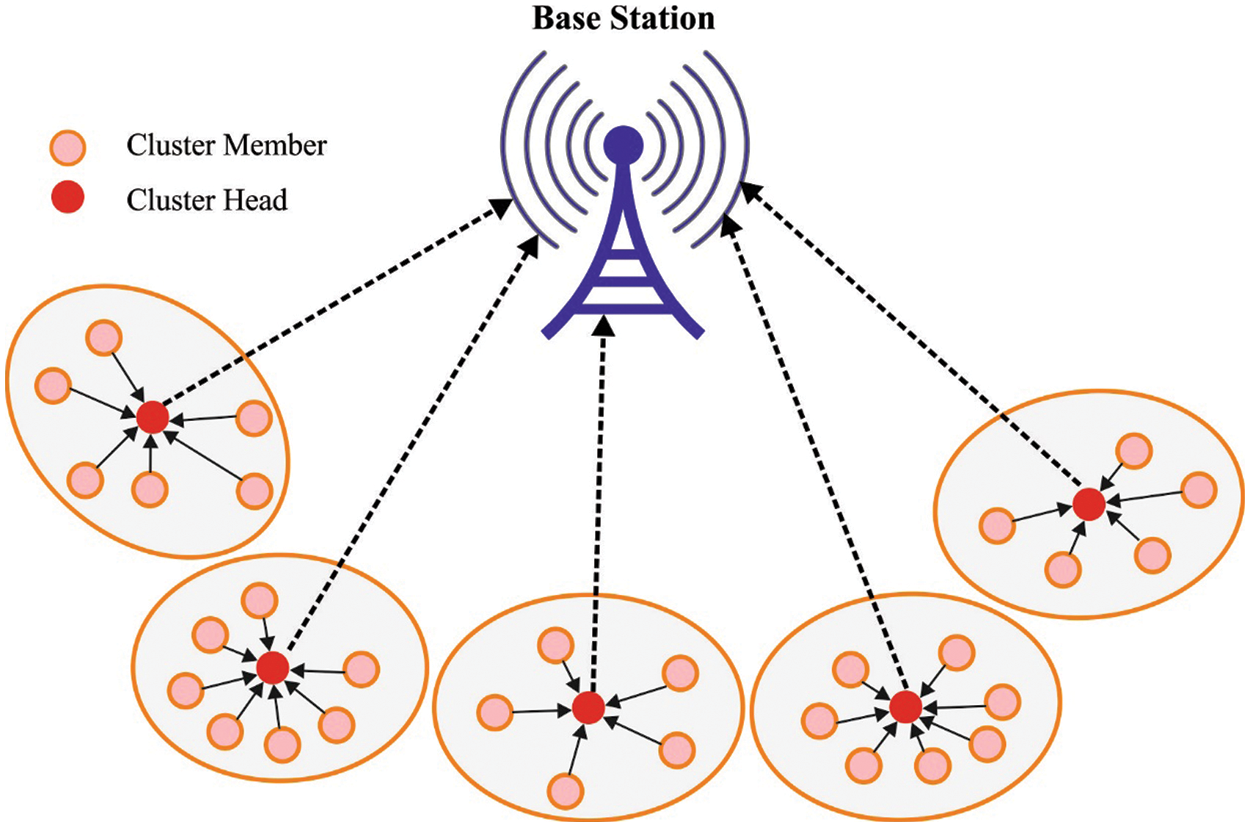
Figure 1: Structure of WSN

Node data might be handled either halfway or in a dispersed way. In concentrated localization, distance estimations are gathered by a focal processor before computation. In appropriated calculations, the sensors share their data just with neighbors yet conceivably iteratively [6]. The two techniques face the significant expense of correspondence, however, by and large, concentrated localization creates more exact area data, though appropriated localization offers greater adaptability and vigor to connect disappointments [7]. NL depends on the estimations of distances between the nodes to be confined and various reference or anchor nodes. Precise area data is significant in practically all genuine utilizations of WSNs. Specifically, localization in a three-layered (3D) space is essential as it yields more precise outcomes. Trilateration and multilateration situating techniques [8] are insightful strategies utilized in two-layered (2D) and three-layered (3D) spaces, individually. These techniques use distance estimations to assess the objective area systematically and experience the ill effects of horrible showing, diminished exactness, and computational intricacy, particularly in the 3D case [9]. All the more explicitly, trilateration is the assessment of node area through distance estimations from three reference nodes with the end goal that the crossing point of three circles is figured, in this manner finding the node [10].

In [11], an enhanced DV-Hop technique dependent upon hop thinning and distance correction was presented. The minimal hop was modified by presenting Received Signal Strength Indication (RSSI) ranging technologies, and the average hop distance was modified by weight average value of hop distance error and evaluated distance errors. Next, the entire enhancement on the place performance of Hop-DV place technique was recognized. In [12], optimized distance range free (ODR) resolves this hop size and after that, a centroid was attained in the minimal far away anchor nodes to unknown nodes. At this point, a minimal probable distance identified as base distance was measured with routing table support. During the final step, the DV-Hop utilizes least square regression for localizing, but ODR exploits linear optimized for comprehending the base distance to localize.

Messous et al. [13] present an enhanced DV-Hop technique in this work. The distance amongst unknown nodes and anchors was evaluated utilizing the RSSI and polynomial approximation. Besides, the presented technique utilizes a recursive computation of localized procedures for improving the accuracy of place estimation. In [14], a new soft computing approach such as Adaptive Plant Propagation Algorithm (APPA) was established for attaining the optimization places of these mobile nodes. These mobile target nodes were heterogeneous and utilized in an anisotropic environment containing an Irregularity (Degree of Irregularity (DOI)) value fixed to 0.01.

This study focuses on the design of Intelligent Aquila Optimization Algorithm Based Node Localization Scheme (IAOAB-NLS) for WSN. The presented IAOAB-NLS model makes use of anchor nodes to determine proper positioning of the nodes. In addition, the IAOAB-NLS model is stimulated by the behaviour of Aquila. The IAOAB-NLS model has the ability to accomplish proper coordinate points of the nodes in the network. For guaranteeing the proficient NL process of the IAOAB-NLS model, widespread experimentation takes place to assure the betterment of the IAOAB-NLS model.

2  Design of IAOAB-NLS Model

In this study, a novel IAOAB-NLS model has been developed for NL in WSN. The presented IAOAB-NLS model makes use of anchor nodes to determine proper positioning of the nodes. In addition, the IAOAB-NLS model is stimulated by the behaviour of Aquila.

2.1 Overview of AO

AO is a population-based method, the heightened rule starts by the population of candidate solution (X) as shown in Eq. (1) that is stochastically formed among the upper bounds(UB) and lower bounds (LB) of the presented issue. The finest solution attained in every round is described by the following [15,16].

x=[x1,1⋯x1,jx1,Dim−1x1,Dimx2,1⋯x2,j⋯x2,Dim⋯⋯xi,j⋯⋯⋮⋮⋮⋮⋮xN−1,1⋯xN−1,j⋯xN−1,DimxN,1⋯xN,jxN,Dim−1xN,Dim](1)

whereas Dim indicates the dimension of the problem, X denotes the collection of existing candidate solutions that can be arbitrarily formed. Xi shows the conclusion value of ith solution and N characterize the total sum of candidate solutions.

Xij=rand×(UBj−LBj)+LBj,i=1,2,…..,Nj=1,2,…,Dim(2)

whereas rand represents the arbitrary value, LBj determines the jth lower bound, and UBj indicates the jth upper bound. The AO method is communication in exploration to exploitation phases using different presentations depending on the form when t≤(23)∗T the exploration phases have been enthusiastic; otherwise, the exploitation phases are executed. Now, the AO explorers in greater soar to determine the region of searching region where the prey is. This presentation can be arithmetically shown below,

X1(t+1)=Xbest(t)×(1−tT)+(XM(t)−Xbest(t)∗rand),(3)

whereas, X1(t+1) indicates the solution of succeeding iteration of t i.e., produced by primary search method (X1). Xbest(t) indicates the optimal achieved solution till tth iteration, this regenerates the assessed prey location. The equation (1−tT) is used to control the extending searching (exploration) with the quantity of rounds. XM(t) describes the place mean value of existing solution related to tth round viz. calculated in the following. rand shows the arbitrary values within [0,1]. r and T demonstrate the existing and the maximal iterations [17].

XM(t)=1N∑i=1NXj(t),∀j=1,2,…,Dim(4)

In which Dim denotes the dimension size of problem and N characterizes the population size.

In the next method (X2), when the prey region is initiated, the Aquila round on the target, arrange the land and follow attacks. This presentation was arithmetically given below.

X2(t+1)=Xbest(t)×Levy(D)+XR(t)+(y−x)∗rand,(5)

Now X2(t+1) indicates the solution of subsequent rounds of r that is produced by the following search technique (X2). D indicates the dimension region, and Levy(D) determines the levy flight distribution function that is calculated. XR(t) characterizes the arbitrary solution attained within at ith rounds.

Levy(D)=s×u×σ|v|1β(6)

Here, s shows the constant value fixed to 0.01, u and v represents the arbitrary values among [0,1]. σ indicates the calculated as follows.

σ=(Γ(1+β)×sine(πβ2)Γ(1+β2)×β×2(β−12))(7)

Then, y and x are employed to present the spiral shape in the search procedure as:

y=r×cos(θ)(8)

x=r×sin(θ)(9)

whereas,

r=r1+U×D1(10)

θ=−ω×D1+θ1(11)

θ1=3×π2(12)

In the third process (X3), when the prey region is perfectly recognized, and the Aquila was organized to land and attack, they vertically incline with opening attack for determining the prey response. This method is termed minimal flight. Fig. 2 shows the process involved in AO algorithm [18]. Currently, the AO exploits the preferred area of the target for receiving near prey and attack. This presentation was arithmetically expressed as.

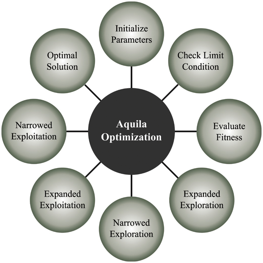
Figure 2: Process involved in AO algorithm [17]

X3(t+1)=(Xbest(t)−XM(t))×α−rand+((UB−LB)×rand+LB)×δ,(13)

In the fourth method (X4), once the Aquila near the prey, the Aquila attacks the prey on the land according to its stochastic motion. This procedure has been arithmetically expressed in the following

X4(t+1)=QF×Xbest(t)−(G1×X(t)×rand)−G2×Levy(D)+rand×G1,(14)

Here X4(t+1) indicates the solution of following iteration of t that was formed by the fourth searching method (X4). QF determines the quality function employed for equilibrium the searching approach that has been calculated.

2.2 Process Involved in IAOAB-NLS Model

The IAOAB-NLS model was executed to estimate the co-ordinate of sensor nodes. An essential purpose of NL in WSN lies in computing the co-ordinate of chosen nodes by minimizing of objective function. IAOAB-NLS model contains the subsequent stages to localize the sensor node from WSN [18]:

•   Uploaded M target nodes (TNs) and N anchor nodes (ANs) randomly from the sensor area. Every ANs are location aware and used for identifying the place of other nodes. Every the AN and TN contain transmitting range R.

•   The distance among the target and ANs were estimated and distinct with additive Gaussian noise. The TN determines the distance as d^i=di+ni whereas di denotes the real distance which is measured among the place of TN (x,y) and place of beacon (xi,yi) utilizing the offered function:

di=(x−xi)2+(y−yi)2(15)

The parameter ni indicates the noise that disturbs the measured distance in di±di(Pn100) in which Pn determines the noise ratio from the expected distance.

•   The desired node was named as localizable node once it contains 3 ANs inside the transmission radius of TN. Next, the reason is dependent upon trilateral positioning model, co-ordinates of 3 ANs (x1,y1), B(x2,y2), and C(x3,y3), and distance among the TN di and 3 ANs are recognized.

•   In event of a localizable node, the IAOAB-NLS model was executed autonomously for recognizing the place of TN. The AO algorithm has been applied to employ the centroid of ANs inside a transmits radius employing the offered function:

(xc,yc)=(1N∑i=1Nxi,1N∑i=1Nyi)(16)

In which N stands for the total amount of ANs inside the transmission range of localizing TN.

•   The IAOAB-NLS model was suitable to identify the co-ordinate (x,y) as TN that reduces the error localization. The primitives executed in localization issue is a mean square distance among the target and AN which is reduced by the application of offered notion:

f(x,y)=1N(∑i=1N(x−xi)2+(y−yi)2−d^)2(17)

whereas N≥3 defines the amount of ANs inside a broadcast radius of TN.

•   Once the highest amount of iterations is reached, then the optimum place co-ordination (x,y) was determined employing IAOAB-NLS model.

•   The whole localization error was defined then estimating the localize TN NL. It can be measured as mean square of distance is determined node co-ordinate (Xi,Yi) from the actual node co-ordinate (xi,yi) is formulated as:

E1=1N1∑i=1N(xi−Xi)2+(yi−Yi)2(18)

•   Steps 2 to 6 obtain repeated still the TNs is localization. The localized method dependent upon the superior error localization E1 and amount of unlocalized nodes NNL is determined as NNL=M−NL. The lesser scores of E1 and NNL signifies the effectual localization procedure.

3  Results and Discussion

In this section, a widespread examination of the IAOAB-NLS model with recent models [18–20] is carried out under distinct aspects such as AN, transmission error (TE), and ranging error (RE). Tab. 1 and Fig. 3 reports a brief number of localized nodes (NOLN) examination of the IAOAB-NLS model under dissimilar ANs. The experimental outcomes implied that the IAOAB-NLS model has gained maximum NOLN under every AN. For instance, with 10 ANs, the IAOAB-NLS model has offered higher NOLN of 135 whereas the GTA-NLS, KH-NLS, GW-NLS, and FF-NLS models have obtained lower NOLN of 126, 118, 105, and 99 respectively. Similarly, with 50 ANs, the IAOAB-NLS model has provided increased NOLN of 194 whereas the GTA-NLS, KH-NLS, GW-NLS, and FF-NLS models have gained decreased NOLN of 176, 161, 144, and 146 respectively.

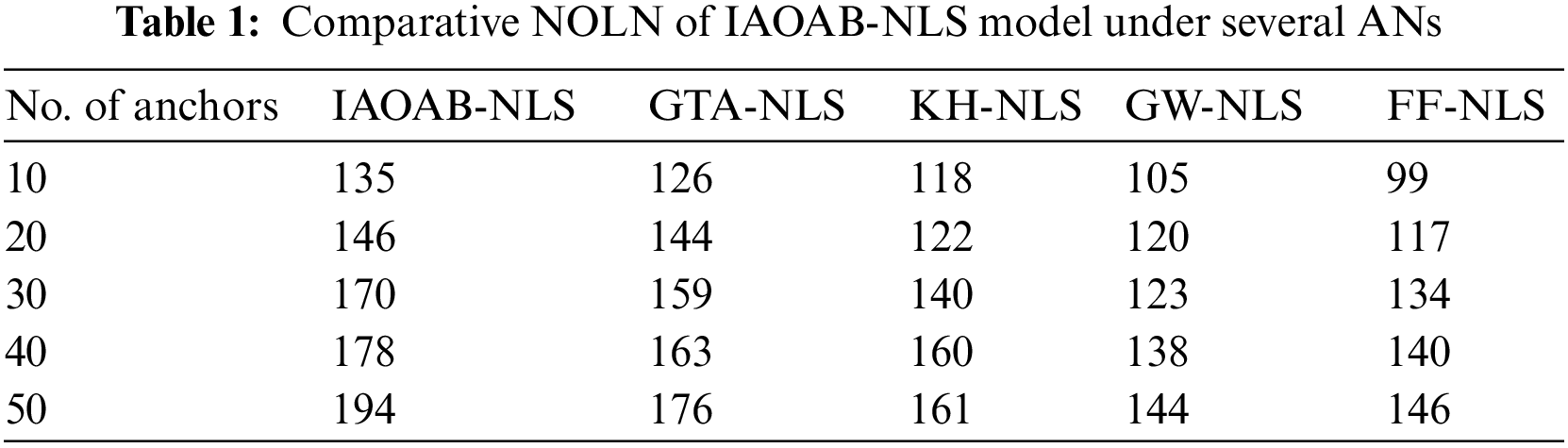
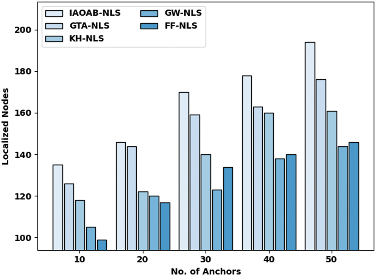
Figure 3: NOLN examination of IAOAB-NLS with recent models

Tab. 2 and Fig. 4 provide a comprehensive localization error (LE) investigation of the IAOAB-NLS model under dissimilar ANs. The experimental outcomes signified that the IAOAB-NLS model has accomplished least LE under every AN. For instance, with 10 ANs, the IAOAB-NLS model has offered reduced LE of 32.50% whereas the GTA-NLS, KH-NLS, GW-NLS, and FF-NLS models have gotten increased LE of 37%, 41%, 47.50%, and 50.50% respectively. Likewise, with 50 ANs, the IAOAB-NLS model has provided least LE of 3% whereas the GTA-NLS, KH-NLS, GW-NLS, and FF-NLS models have gained increased NOLN of 12%, 19.50%, 28%, and 27% respectively.

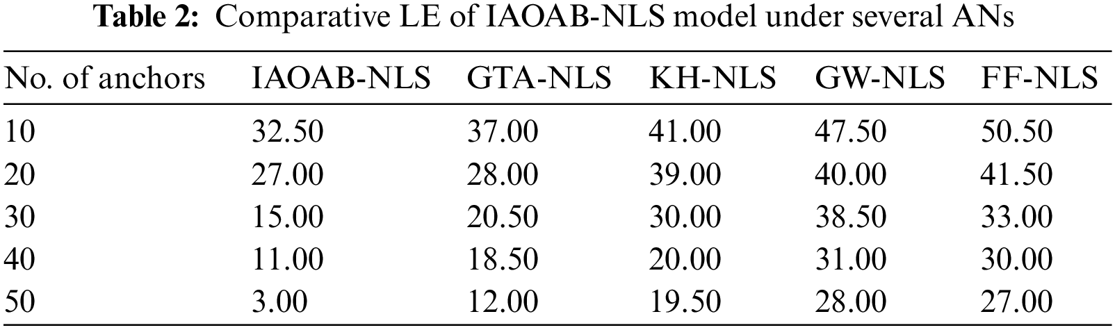
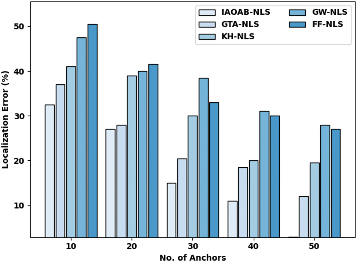
Figure 4: LE examination of IAOAB-NLS with recent models

Tab. 3 and Fig. 5 study a detailed localization rate (LR) inspection of the IAOAB-NLS model under divergent ANs. The investigational outcomes inferred that the IAOAB-NLS model has extended maximum LR under every AN. For instance, with 10 ANs, the IAOAB-NLS model has presented greater LR of 67.50% whereas the GTA-NLS, KH-NLS, GW-NLS, and FF-NLS models have attained lesser NOLN of 63%, 59%, 52.50%, and 49.50% respectively. Likewise, with 50 ANs, the IAOAB-NLS model has provided increased NOLN of 97% whereas the GTA-NLS, KH-NLS, GW-NLS, and FF-NLS models have gained decreased NOLN of 88%, 80.50%, 72%, and 73% respectively.

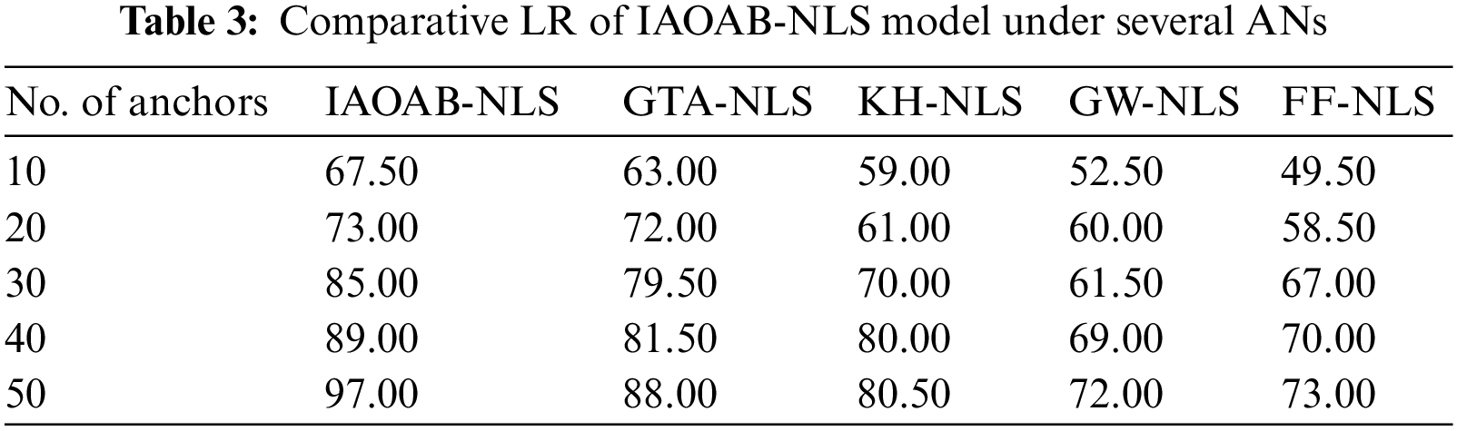
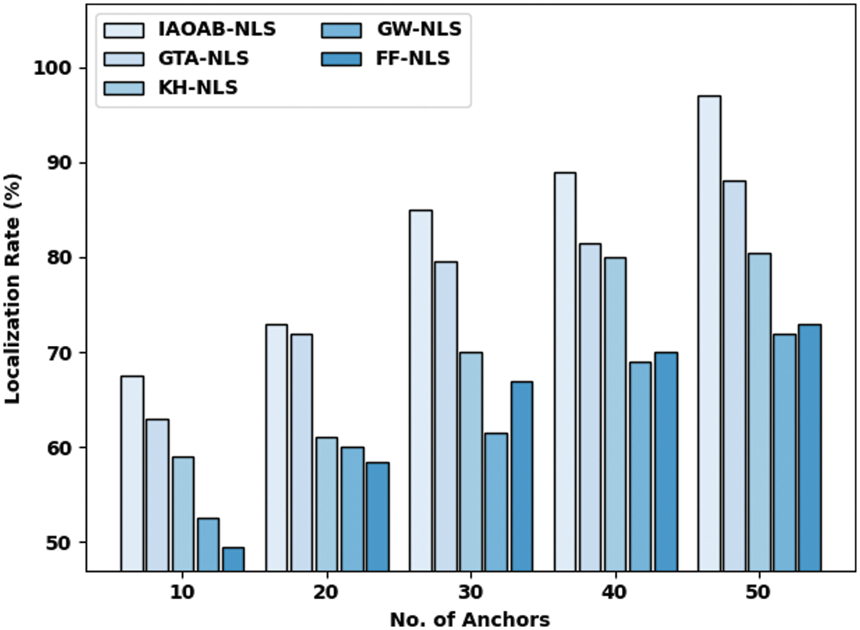
Figure 5: LR examination of IAOAB-NLS with recent models

Tab. 4 and Fig. 6 offer an inclusive LE exploration of the IAOAB-NLS model under dissimilar RE. The experimental outcomes implied that the IAOAB-NLS model has gifted least LE under every AN. For instance, with 5% of REs, the IAOAB-NLS model has offered reduced LE of 29.47% whereas the GTA-NLS, KH-NLS, GW-NLS, and FF-NLS models have gotten increased LE of 39.39%, 68.33%, 44.78%, and 66.93% respectively.

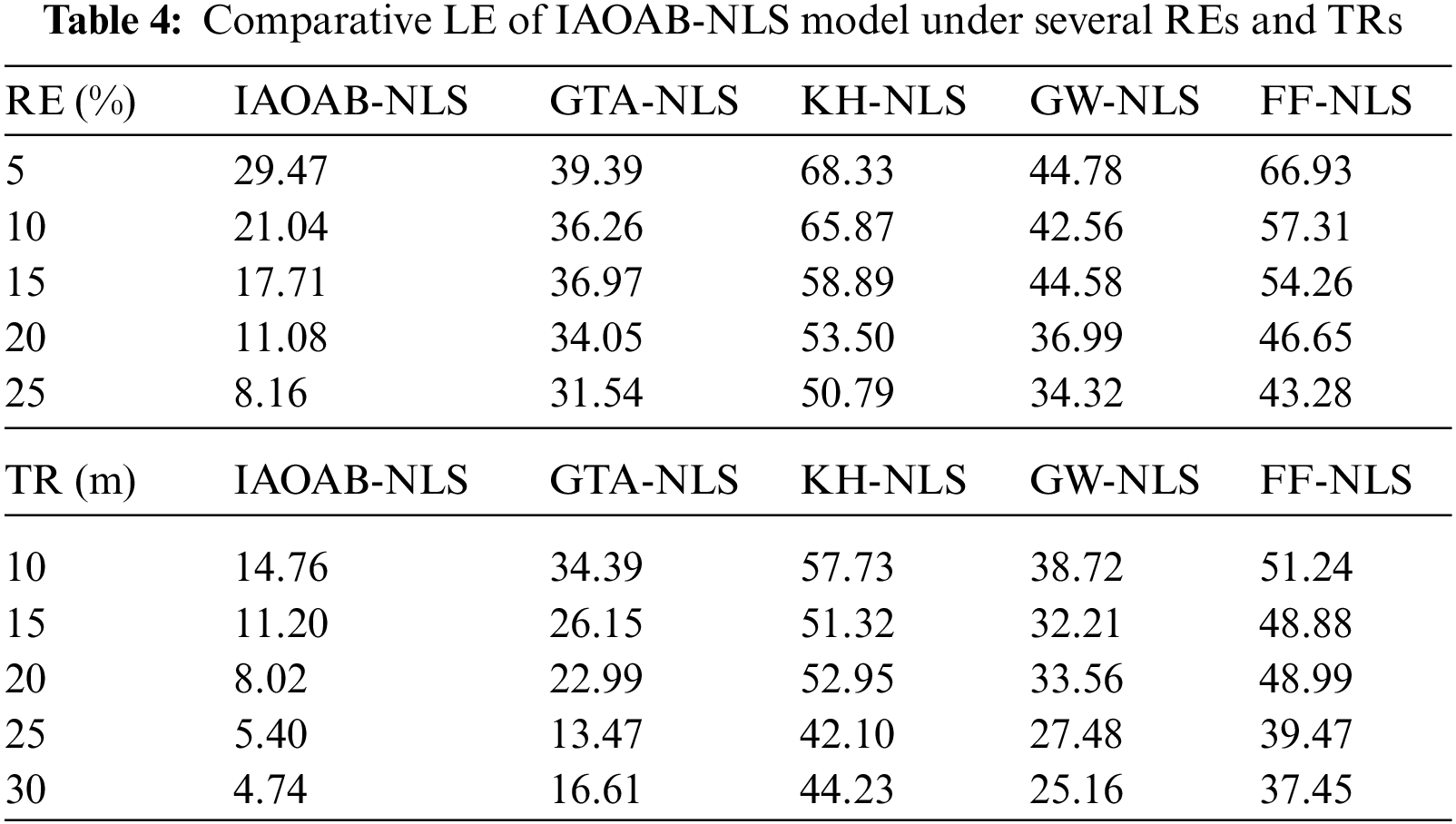
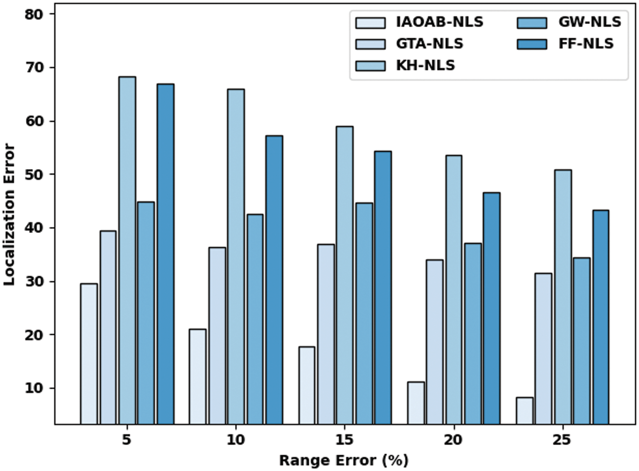
Figure 6: LE examination of IAOAB-NLS model under several REs

Then, with 10% of REs, the IAOAB-NLS model has offered reduced LE of 21.04% whereas the GTA-NLS, KH-NLS, GW-NLS, and FF-NLS models have gotten increased LE of 36.26%, 65.873%, 42.56%, and 57.31% respectively.

At last, with 15% of RE, the IAOAB-NLS model has provided least LE of 17.71% whereas the GTA-NLS, KH-NLS, GW-NLS, and FF-NLS models have gained increased NOLN of 36.97%, 58.89%, 44.58%, and 54.26% respectively. Eventually, with 25% of RE, the IAOAB-NLS model has provided least LE of 8.16% whereas the GTA-NLS, KH-NLS, GW-NLS, and FF-NLS models have gained increased NOLN of 31.54%, 50.79%, 34.32%, and 43.28% respectively.

Finally, Fig. 7 delivers a complete LE investigation of the IAOAB-NLS model under dissimilar TR. The experimental outcomes directed that the IAOAB-NLS model has accomplished least LE under every AN. For instance, with 10TR, the IAOAB-NLS model has offered reduced LE of 14.76% whereas the GTA-NLS, KH-NLS, GW-NLS, and FF-NLS models have gotten increased LE of 34.39%, 57.73%, 38.72%, and 51.24% respectively. Moreover, with 15 TR, the IAOAB-NLS model has provided least LE of 11.20% whereas the GTA-NLS, KH-NLS, GW-NLS, and FF-NLS models have gained increased NOLN of 26.15%, 51.32%, 32.21%, and 48.88% respectively. Furthermore, with 20 TR, the IAOAB-NLS model has provided least LE of 8.02% whereas the GTA-NLS, KH-NLS, GW-NLS, and FF-NLS models have gained increased NOLN of 22.99%, 52.95%, 33.56%, and 48.99% respectively. In line with, under 25 TR, the IAOAB-NLS model has provided least LE of 5.40% whereas the GTA-NLS, KH-NLS, GW-NLS, and FF-NLS models have gained increased NOLN of 13.47%, 42.10%, 27.48%, and 39.47% respectively.

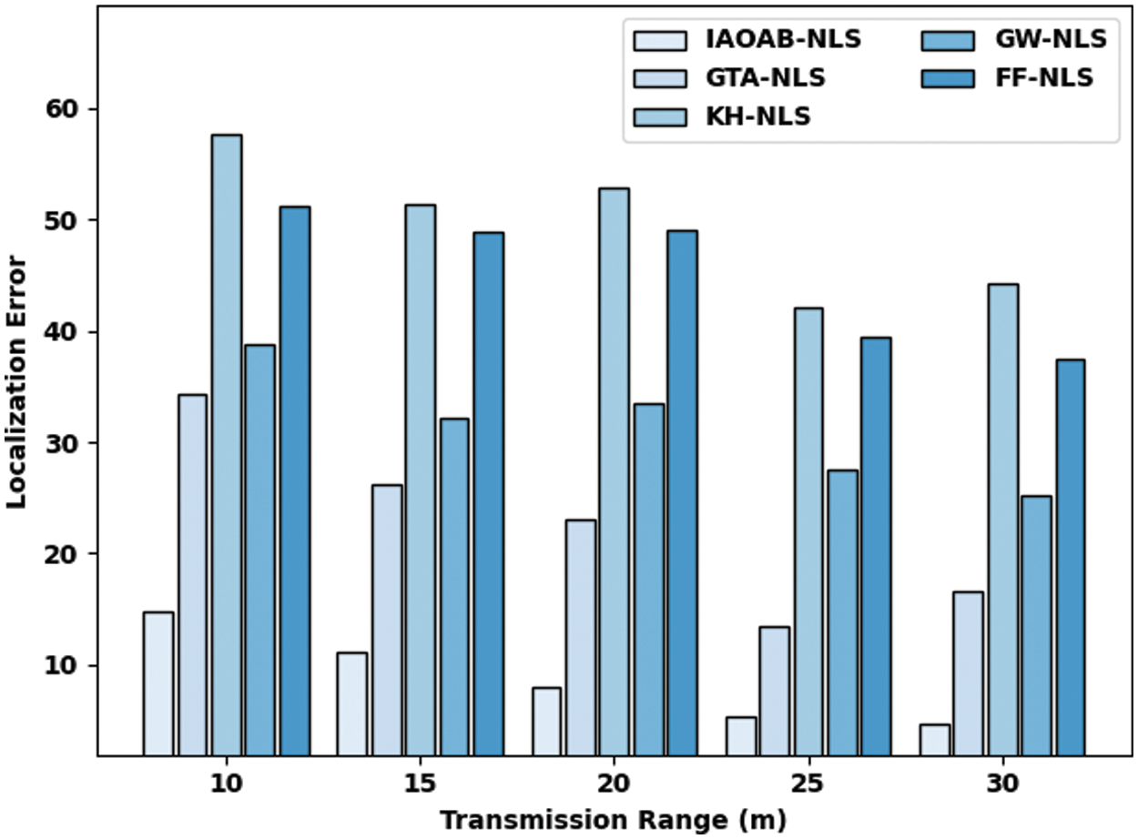
Figure 7: LE examination of IAOAB-NLS model under several REs and TRs

Equally, with 30 TR, the IAOAB-NLS model has provided least LE of 4.74% whereas the GTA-NLS, KH-NLS, GW-NLS, and FF-NLS models have gained increased NOLN of 16.61%, 44.23%, 25.16%, and 37.45% respectively.

The above mentioned experimental outcome pointed out that the IAOAB-NLS model has outperformed other models in accomplishing superior NL outcomes in WSN.

4  Conclusion

In this study, a novel IAOAB-NLS model has been developed for NL in WSN. The presented IAOAB-NLS model makes use of anchor nodes to determine proper positioning of the nodes. In addition, the IAOAB-NLS model is stimulated by the behaviour of Aquila. The IAOAB-NLS model has the ability to accomplish proper coordinate points of the nodes in the network. For guaranteeing the proficient NL process of the IAOAB-NLS model, widespread experimentation takes place to assure the betterment of the IAOAB-NLS model. The resultant values reported the effectual outcome of the IAOAB-NLS model irrespective of changing parameters in the network. Thus, the IAOAB-NLS model can appear as a novel tool for precise NL in the network. In future, hybrid AOA can be derived by the use of local searching techniques.

Funding Statement: The authors extend their appreciation to the Deanship of Scientific Research at King Khalid University for funding this work under Grant Number (RGP 1/322/42). Princess Nourah bint Abdulrahman University Researchers Supporting Project number (PNURSP2022R303), Princess Nourah bint Abdulrahman University, Riyadh, Saudi Arabia.

Conflicts of Interest: The authors declare that they have no conflicts of interest to report regarding the present study.

References

 1.  Y. Robinson, S. Vimal, E. Julie, K. L. Narayanan and S. Rho, “3-dimensional manifold and machine learning based localization algorithm for wireless sensor networks,” Wireless Personal Communications, vol. 77, no. 3, pp. 1, 2021. [Google Scholar]

 2.  S. Arjunan and S. Pothula, “A survey on unequal clustering protocols in Wireless Sensor Networks,” Journal of King Saud University - Computer and Information Sciences, vol. 31, no. 3, pp. 304–317, 2019. [Google Scholar]

 3.  J. Qiao, J. Hou, J. Gao and Y. Wu, “Research on improved localization algorithms RSSI-based in wireless sensor networks,” Measurement Science and Technology, vol. 32, no. 12, pp. 125113, 2021. [Google Scholar]

 4.  S. Arjunan and P. Sujatha, “Lifetime maximization of wireless sensor network using fuzzy based unequal clustering and ACO based routing hybrid protocol,” Applied Intelligence, vol. 48, no. 8, pp. 2229–2246, 2018. [Google Scholar]

 5.  J. Uthayakumar, T. Vengattaraman and P. Dhavachelvan, “A new lossless neighborhood indexing sequence (NIS) algorithm for data compression in wireless sensor networks,” Ad Hoc Networks, vol. 83, no. 2009, pp. 149–157, 2019. [Google Scholar]

 6.  S. Arjunan, S. Pothula and D. Ponnurangam, “F5N-based unequal clustering protocol (F5NUCP) for wireless sensor networks,” International Journal of Communication Systems, vol. 31, no. 17, pp. e3811, 2018. [Google Scholar]

 7.  S. Famila, A. Jawahar, A. Sariga and K. Shankar, “Improved artificial bee colony optimization based clustering algorithm for SMART sensor environments,” Peer-to-Peer Networking and Applications, vol. 13, no. 4, pp. 1071–1079, 2020. [Google Scholar]

 8.  W. Sun, L. Dai, X. R. Zhang, P. S. Chang and X. Z. He, “RSOD: Real-time small object detection algorithm in UAV-based traffic monitoring,” Applied Intelligence, vol. 92, no. 6, pp. 1–16, 2021. [Google Scholar]

 9.  W. Fang, W. Zhang, L. Shan, B. Assefa and W. Chen, “Ldpc code’s decoding algorithms for wireless sensor network: A brief review,” Journal of New Media, vol. 1, no. 1, pp. 45–50, 2019. [Google Scholar]

10. T. K. Mohanta and D. K. Das, “Advanced localization algorithm for wireless sensor networks using fractional order class topper optimization,” The Journal of Supercomputing, vol. 78, no. 8, pp. 10405–10433, 2022. [Google Scholar]

11. D. Xue, “Research of localization algorithm for wireless sensor network based on DV-Hop,” EURASIP Journal on Wireless Communications and Networking, vol. 2019, no. 1, pp. 218, 2019. [Google Scholar]

12. S. Kumar, S. Kumar and N. Batra, “Optimized distance range free localization algorithm for WSN,” Wireless Personal Communications, vol. 117, no. 3, pp. 1879–1907, 2021. [Google Scholar]

13. S. Messous, H. Liouane, O. Cheikhrouhou and H. Hamam, “Improved recursive dv-hop localization algorithm with rssi measurement for wireless sensor networks,” Sensors, vol. 21, no. 12, pp. 4152, 2021. [Google Scholar]

14. G. S. Walia, P. Singh, M. Singh, M. Abouhawwash, H. J. Park et al., “Three dimensional optimum node localization in dynamic wireless sensor networks,” Computers, Materials & Continua, vol. 70, no. 1, pp. 305–321, 2022. [Google Scholar]

15. L. Abualigah, D. Yousri, M. A. Elaziz, A. A. Ewees, M. A. A. Al-qaness et al., “Aquila optimizer: A novel meta-heuristic optimization algorithm,” Computers & Industrial Engineering, vol. 157, no. 11, pp. 107250, 2021. [Google Scholar]

16. A. M. AlRassa, M. A. A. Al-qaness, A. A. Ewees, S. Ren, M. A. Elaziz et al., “Optimized ANFIS model using aquila optimizer for oil production forecasting,” Processes, vol. 9, no. 7, pp. 1194, 2021. [Google Scholar]

17. M. R. Hussan, M. I. Sarwar, A. Sarwar, M. Tariq, S. Ahmad et al., “Aquila optimization based harmonic elimination in a modified h-bridge inverter,” Sustainability, vol. 14, no. 2, pp. 929, 2022. [Google Scholar]

18. P. Sekhar, E. L. Lydia, M. Elhoseny, M. A. Akaidi, M. M. Selim et al., “An effective metaheuristic based node localization technique for wireless sensor networks enabled indoor communication,” Physical Communication, vol. 48, no. 6, pp. 101411, 2021. [Google Scholar]

19. L. Singh, A. K. Singh and P. K. Singh, “Secure data hiding techniques: A survey,” Multimedia Tools and Applications, vol. 79, no. 23–24, pp. 15901–15921, 2020. [Google Scholar]

20. Y. Kumar and P. K. Singh, “Improved cat swarm optimization algorithm for solving global optimization problems and its application to clustering,” Applied Intelligence, vol. 48, no. 9, pp. 2681–2697, 2018. [Google Scholar]