Vehicle Plate Number Localization Using Memetic Algorithms and Convolutional Neural Networks

1  Introduction

Automatic license plate recognition (ALPR) is a basic component of Intelligent Transportation Systems (ITS) which is an essential system in smart cities. ALPR has many applications such as law enforcement, surveillance, and toll booth operations [1]. ALPR systems can be categorized into four classes depending on the type of the basic primitive on which the detection algorithm is based. These categories are color-based, edge-based, texture-based, and character-based. Color-based systems scan the unknown image to find a candidate window that contains an image with color properties similar to the targeted License Plate (LP). The similarity between the image window and the prototype is detected by many different techniques either through direct correlation or through histogram-based methods to overcome illumination problems [2]. Genetic algorithms also have been used to do a heuristic search for this similarity to identify the license plate color [3]. Edge-based techniques depend on the fact that the area of the LP has a high density of small edges either vertical, horizontal, or inclined [4] because of its inclusion of many alphanumeric symbols that represent the license number in addition to the LP rectangular bounding box. Edge-based techniques require the use of a fast edge-detection algorithm [5]. Texture-based techniques can be considered an extension of the edge-based techniques because they depend on the presence of the characters in the plate area which creates a unique pixel intensity distribution inside the plate region. Special methods were used to localize the LP textures such as Vector Quantization [6] and Gabor filter [7]. Character-based techniques [8,9] mostly depend on the connected component analysis (CCA) technique that detects the LP symbols based on the pixels’ connectivity after converting the image into binary. The success of these character-based techniques relies mainly on the binarization step which is affected by the illumination conditions’ variations and the physical distortions caused by aging or inaccurate fixing of the LP that cause the license symbols to be connected to each other or to the license frame. The techniques used in LP detection vary from simple matching methods to machine learning and finally deep learning techniques. The best success has been achieved using deep learning techniques where training is carried out on a huge number of image samples that cover all the expected variations of geometric and illumination conditions. Deep learning techniques deal with the LP detection problem as an object detection problem. Different types of deep learning architectures have been used to perform localization and even recognition. The state-of-the-art real-time object detectors such as Convolutional neural networks (CNN) with region proposals (Faster R-CNN) [10], You-Only-Look-Once (YOLO 9000) [11] and Single-Shot-Detection (SSD300) [12] have achieved real-time detection of the LP position. End-To-End license plate detection and recognition using deep neural networks (Towards end-to-end (TE2E)) [13] has shown high detection accuracy by training a single neural network architecture to do detection and recognition at the same time. An End-To-End architecture called the Roadside Parking Net (RPnet) [14] achieved higher speed and accuracy on the CCPD challenging dataset (CCPD). A comprehensive review of the problems and the different techniques used in LP detection and recognition is found in [1]. Although recently, the most accurate techniques in LP detection and recognition are based on deep learning models, these techniques are highly dependent on being trained on a huge number of labelled datasets and need retraining of these models for new symbols or LP layouts. Unlike the huge amount of training datasets and the large number of the model parameters needed in the deep learning-based solutions, in [15], we have introduced a genetic algorithm (GA)-based technique that depends only on a simple geometric representation of the symbols layout of the concerned plate that has a number of parameters not more than 4 × L2 where L is the number of LP symbols and all these parameters are stored in a geometrical relationship matrix (GRM). An important metric that should be taken into consideration when evaluating systems or techniques is the number of instances needed to do the training and the length of the training time. In [15], only one clear instance of an LP image is required to produce the GRM in a period less than one second. This is very important if we consider for example a robot (or auto-driving vehicle) that is required to track a foreign vehicle with a different plate layout in an emergent condition. In this case, the learning time is the most important factor which makes us conclude that future research should concentrate on machine learning techniques as well as deep learning techniques, and old techniques such as k-nearest neighbor or even simple matching techniques should not be neglected because they possess the feature of instant learning. In the previous versions of the GA-based technique [15–17], most illumination problems have been tackled by using local adaptive binarization methods especially in [17]. Unlike almost all systems that use a single binarization technique, in this research a deeper and more general solution is founded by applying different binarization techniques in parallel and combining their outputs to produce a larger solution space of connected components objects (CCOs) to increase the detection probability. Since having many CCOs will increase the computational complexity, object based and neighborhood adaptive filtering stages are applied to minimize the number of CCOs and hence speed up the computation and at the same time minimize the false positive (FP) solutions. Although most ALPR systems are performed in three steps (LP detection, LP segmentation, and LP symbols recognition) except End-To-End techniques [1], the GA-based technique, introduced initially in [15] and enhanced in [16] to support inclined plates combines the first two steps in one-step. In ALPR systems based on the connected component analysis technique (CCAT), the accuracy and performance are significantly dependent on the binarization stage where each pixel in the image is decided to belong either to the background or to the foreground objects. In [15], an adaptive local binarization stage has been adopted to overcome illumination changes in addition to the skipping ability introduced in the GA to overcome physical problems affecting the CCA technique. The concept of skipping was introduced in [15] and enhanced in [16] to support partial detection of the LP based on the detection of a number of license symbols less than the defined number of symbols in the LP (L). In [17], a novel multi-window-size binarization technique was introduced to support application-independent localization of the license plates. Applying the previous GA-based [15–17] techniques to a recent challenging data set such as the CCPD dataset [14] raises new concerns related to the large number of CCOs produced by the different binarization techniques that are used to overcome illumination and perspective variations of the relatively high-resolution images. To speed up the evolutionary-based technique introduced in [15–17], a memetic operator is introduced in this research to do fast local tuning of the intermediate solutions during the evolutionary iterations. In addition to the enhancement introduced in the object filtering and the evolutionary-based technique, the CCA algorithm is re-implemented to produce the x-y positions and width-height values of every CCO in a wide-angle range (from −85° to 85°). This allows the calculation of the objective distance of any candidate solution based on a horizontal license plate prototype representation without resorting to doing a rotation of either the unknown plate or the prototype and produces more accurate objective distances than the previous implementations. A complete overview of the new system will be introduced in Section 2. The image-processing phase is summarized in Section 3 with a detailed description of the binarization techniques. The new methods for the object filtering phase are described in Section 4. In Section 5, the GA enhancements are described in detail. In Section 6, fake detection using a deep CNN (DCNN) is presented. Finally, the results are presented and discussed in Section 7 and the conclusion is given in Section 8.

2  System Overview

The proposed LP symbols detection system is composed of four phases and each phase is composed of many stages as shown in Fig. 1. In the first phase, the LP image is binarized and a large number (N) of CCOs are produced using three different binarization techniques. Then, in the objects filtering phase many non-LP symbols are filtered out to produce less number (M) and hence reduce the computation and FP candidates. In the third phase, the memetic algorithm (MA) searches the CCOs space for the best sequence that matches the layout of the LP symbol sequence represented by the GRM. FP candidate sequences output by the memetic algorithm are detected in the fourth phase by a deep convolutional neural network DCNN if the objective distance is more than 1 otherwise the output sequence is accepted. A maximum of four trials are required in the worst case to overcome the image processing problems related to the CCA technique and to avoid FP candidates. In the first trial, only the first binarization technique is applied with a window size of 15. In the following three trials, the three binarization techniques are applied with different window sizes as will be shown in the binarization stage. Each of the three trials is initiated if the output of the previous trial is rejected by the DCNN. After the fourth trial, if the best solution so far has an objective distance (OD) less than 6 it is accepted otherwise a plate miss is reported. Most of the system phases and their stages implemented in the previous versions [15–17] are enhanced (highlighted with blue color) and supported with novel additions (highlighted with red color) to increase the accuracy and speed as described in detail in the following sections.

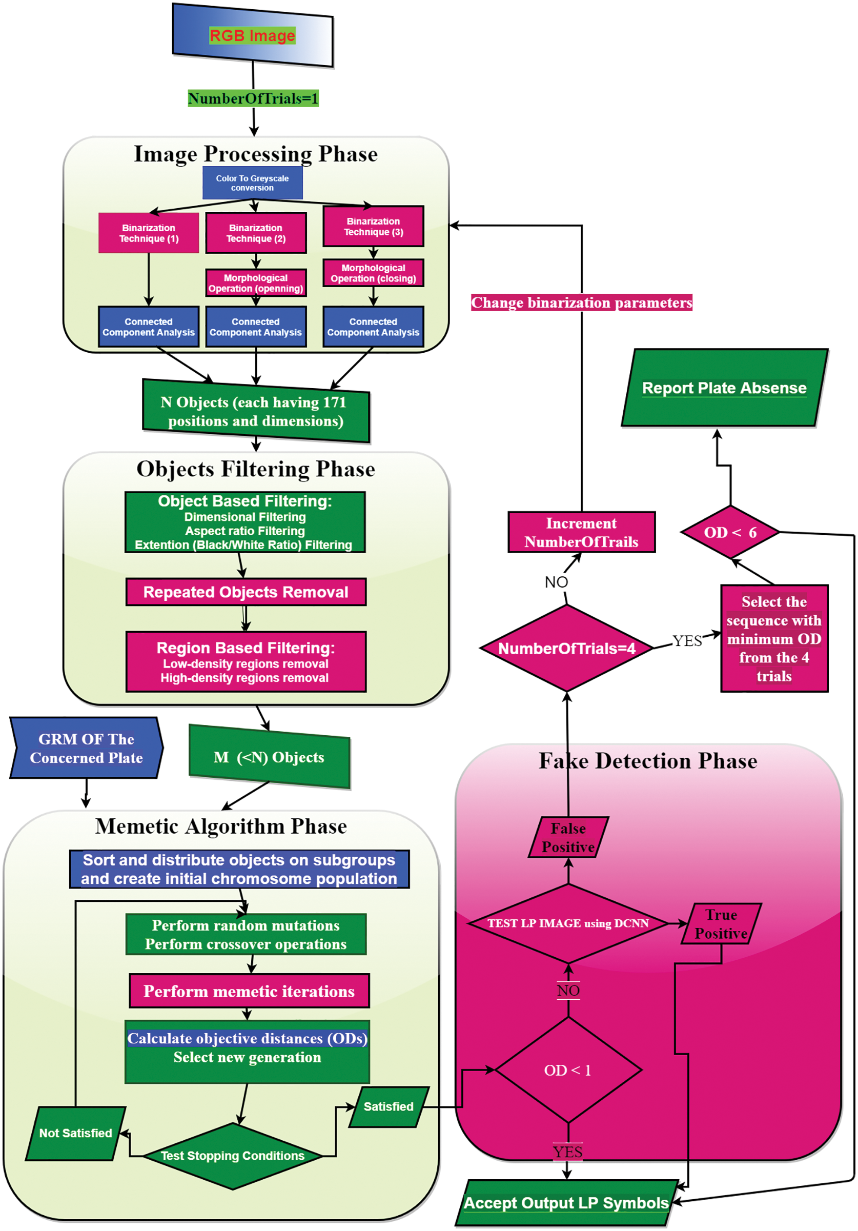
Figure 1: The system’s overall flowchart for the localization of LP symbols where new additions are indicated with a red color and enhanced stages with a blue color

3  Image Processing Phase

In this phase, an input color image is subjected to four stages to extract a number N of foreground objects. These four stages (Color-to-Grey Conversion, Adaptive Binarization, Morphological Operations (optional), and Connected Component Analysis (CCA) are different than those in the previous versions [15–17]. The changes are demonstrated in the following subsections.

3.1 Color-to-Grey Conversion

Unlike most of the work that deals with LP detection that uses the traditional color-to-grey formula [15], the RGB image is converted into grey by summing up the red and green channels only. The blue channel is neglected because the background of the license plate in the tested dataset [14] is blue. Hence, the contrast between the LP symbols and the LP background will be increased. This does not mean that the technique is based on the LP color, but most of the state-of-the-art works that resulted in distinctive accuracy were using the color images without conversion into grey. Hence to compete with these state-of-the-art techniques color is considered in the first stage and in the final fake detection phase when using the DCNN to detect FP solutions. The following formula is used to do the color-to-grey conversion:

GI=0.5 RC+0.5 GC(1)

where RC and GC are the red and green components stored in the red and green channels respectively. GI is the output greyscale image which is normalized to contain values from 0 to 1.

3.2 Multi Adaptive Binarization Techniques Stage

In the first trial, the system performs binarization using a fixed-size window binarization method based on the Nick technique [18]. The Nick technique is built initially to binarize text documents.

In the Nick method, the local threshold LT (x, y) is computed based on the mean m (x, y) and the sum of the squares of pixel intensities inside a local window centered at the current point GI (x, y) using the following formula:

LT(x,y)=m(x,y)+k1.(∑GI(x,y)2−m(x,y)2)/NP(2)

where NP is the number of pixels in the local window and k1 is a parameter ranging from −0.2 to −0.1, but in this research, the selected value of k1 is 0.11.

The second binarization technique is called Niblack [19], which calculates the adaptive threshold LT (x, y) at the current point (x, y), based on the local mean m (x, y) of the intensity around the current point GI (x, y) and the standard deviation δ (x, y) inside the local window as follows:

LT(x,y)=m(x,y)+k2.δ(x,y)(3)

where k2 is a parameter having a selected value of −0.2 in [19], but in this research k2 is equal to −0.11. I noticed that while the threshold in the case of the Nick method is above the mean (due to the selected positive constant (k1)), in the Niblack method it is below the mean, so I consider that the two methods complement each other.

The third binarization technique introduced by Singh et al. [20] calculates the adaptive threshold LT (x, y) at the current point (x, y), based on the local mean m (x, y) of the intensity of the window around the current point and the mean deviation of the current point (dev = IM (x, y) − m (x, y)) as follows

LT(x,y)=m(x,y)[1+k(dev1−dev−1)](4)

where k = 0.06. In this research, a different expression is inspired from the above formula as follows:

LT(x,y)=m(x,y)+0.3×adev×(0.5+adevadev−1)+k3(5)

where adev = average | IM (x, y) − m (x, y) | and k3 is a control parameter in the range [0 0.1]. Unlike Niblack and Nick’s methods, in the new method that we refer to as “Delta”, the threshold may be above or below the (mean) depending on the value of adev and k3. In the case of k3 = 0.06, if adev is greater than 0.48 (approximately) the threshold will be below the mean else it will be above or equal to the mean. In this research, the selected value of k3 is 0.06. In the first trial, the Nick method is applied with a window-side length of 15. The window lengths of the Delta, Niblack and Nick methods for the next three trails are [10, 15, 60], [20, 30, 40], and [30, 60, 15] respectively.

The reason for selecting the above three binarization techniques is their fast and complementary effects based on trial and error.

3.3 Morphological Operations

Since the adaptive filters may produce connected characters, it is sometimes helpful to use the opening operation to separate the connected characters. In this research, I perform an erosion (or open) operation for the output of the Niblack filter using a vertical structuring element of size equal to one-third of the window length (WL/3). Due to the composition of the Chinese character of 2 or more CCOs, a dilation (or close) operation is performed using a horizontal structuring element of size equal to one fifth the window length (WL/5) after the Delta technique to unify the Chinese symbol and at the same time to connect broken symbols. Fig. 2 shows examples of the outputs of the three techniques and the morphological operations for four RGB images taken from the CCPD Blur and FN sections, where each technique contributes differently to the output pool based on the complexity of the input image. If there is a missing object it will be skipped by the MA and its position and dimensions are calculated geometrically based on the GRM.

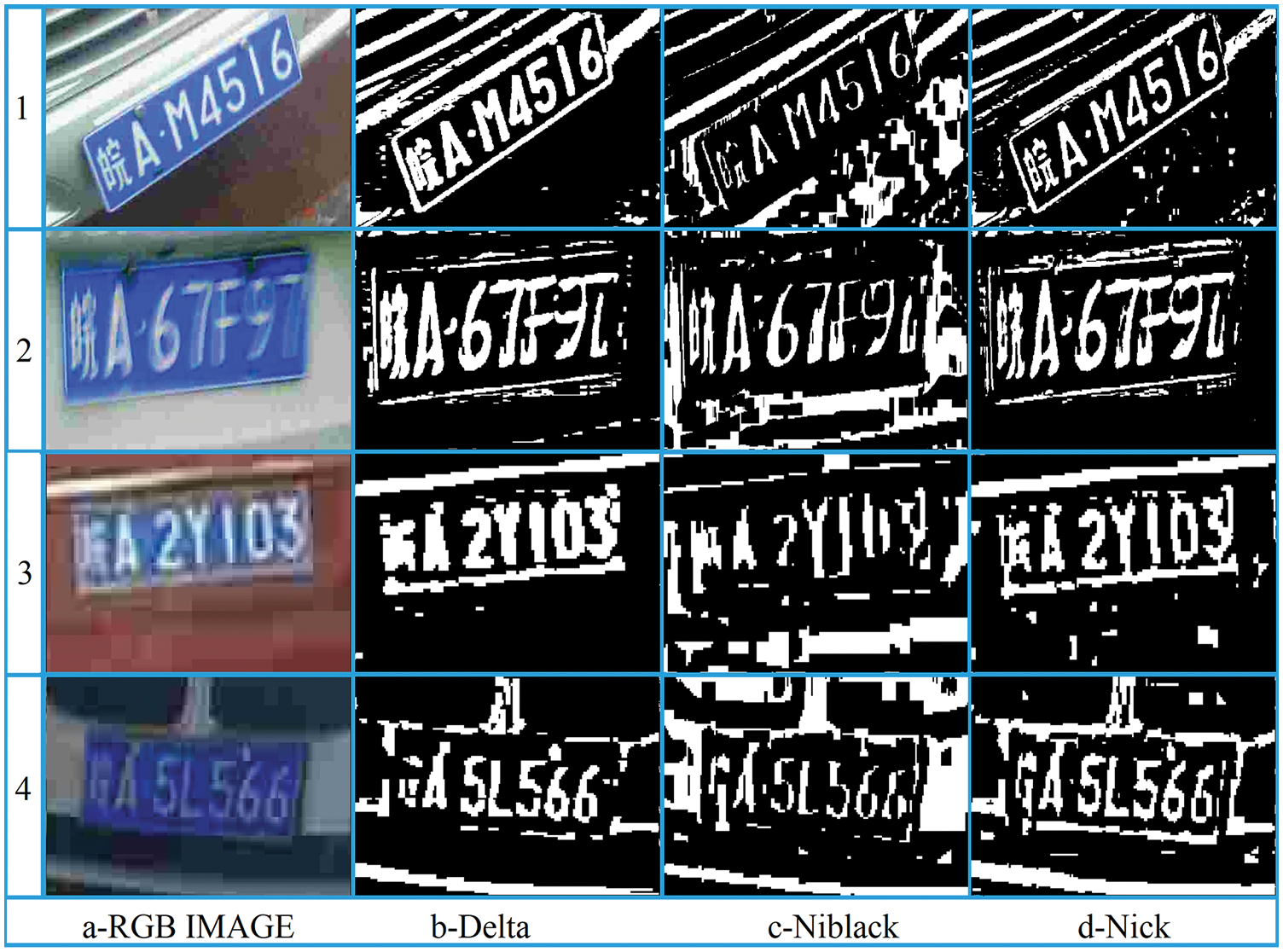
Figure 2: The output of the three binarization techniques Delta, Niblack, and Nick for four RGB input images. Cases 1 and 2 from FN, window size 30 × 30. Cases 3 and 4 from blur, window size 15 × 15

3.4 Connected Component Analysis Stage

In this research, 4-connected component objects are detected, and their bounding boxes parameters are calculated relative to a rotating axis (from −85° to +85°). This allows using the exact dimensions of each object when it is included in a chromosome having a sequence of objects that have an inclined direction without resorting to rotating the prototype template or the sequence of objects themselves to obtain accurate objective distances as shown in Fig. 3 where the dimensions of the red rectangles will be used in calculating the objective distance at 45° angle.

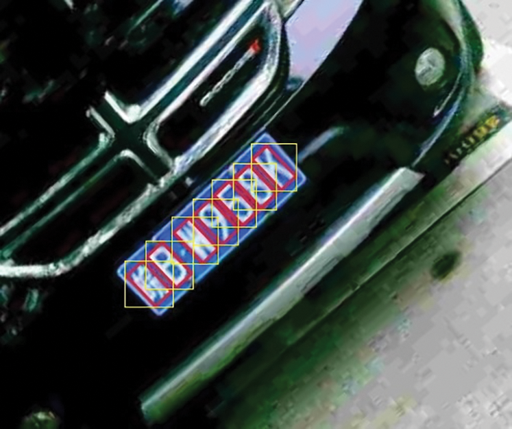
Figure 3: The red rectangles are detected based on a rotated axis of 45° while the yellow rectangles are detected based on the original X-Y axis

4  Objects Filtering Phase

Objects filtering is carried out through three stages. The first stage filters out objects based on their properties (width, height, aspect ratio (Asp), and extension (Ext)). Where the extension is the number of foreground pixels divided by the object area. The second stage removes repeated objects. The third stage is region-based filtering which depends on the distribution of objects around each object.

4.1 Object-Based Filtering

Assuming the image width is ImageWidth, then the maximum width of an object (MaxW) is equal to ImageWidth/L; where L is the number of license plate symbols. The maximum height (MaxH) of an object is (2 × MaxW) and the minimum object width is 3 pixels, considering thin numbers such as ‘1’. The minimum object height (MinH) is 15 pixels. The minimum extension is 0.13. Objects should satisfy the mentioned properties in addition to the following logical condition:

0.3<Asp<3if Ext>0.8(for normal symbols)

Or Asp<=0.3if Ext>0.42(for thin symbols such as‘1′)(6)

4.2 Repeated Objects Removal

Any two objects (j1 and j2) having similarity in their coordinates (X, Y) and dimensions (W, H) are unified which means only one of them is retained and the other is removed where the similarity (S) is given by the following logical expression:

S(j1,j2)=(|Xj1−Xj2|Wavg<0.05)AND(|Yj1−Yj2|Havg<0.05)AND(|Wj1−Wj2|Wavg<0.05)AND(|Hj1−Hj2|Havg<0.05)(7)

where Wavg = (Wj1+Wj2)/2 and Havg=(Hj1+Hj2)/2.

4.3 Region-Based Filtering

This stage depends on the distribution of objects over two sizes of square areas, small-size squares, and large-size squares. Small-size squares are of size 10 × 10. Large size squares have a size of V × V, where V is estimated based on the average object width (Wavg) of all the detected objects (M) and the number of symbols in an LP (L) as follows:

V=(L−1)×Wavg+1(8)

Then we create two matrices each having a number of cells equal to the number of squares in the image, one for the small squares and the other for the large squares. Every object is assigned to its corresponding cell in the two matrices based on its X and Y position and each cell of both matrices contains the number of belonging objects. The integral matrix is calculated for the small-size matrix.

Because symbols in an LP are located near each other and there is a semi-fixed spacing between every two consecutive symbols and this spacing is related to the average width of the symbols, then each LP symbol should have at least 3 neighbor symbols around it if we define the symbol’s neighborhood as the square area that surrounds the symbol and have dimensions NR × NR where NR = 6 × W and W is the actual width of the current object. Hence using the integral matrix, we can estimate the number of objects in the neighborhood square of each object and hence remove the object if its neighborhood square contains less than 3 objects. This condition considers the extreme left or right objects in the LP symbols. The middle objects’ neighborhoods surely will contain more than 2. By applying this condition, we can remove objects existing in low-density regions.

Objects in very high-density regions are removed based on the large-size squares matrix by removing objects that belong to cells having more than 3 × (L + 3) objects (because we have CCOs output from three binarization techniques and the Chinese symbol may be composed of two or more CCOs).

5  MA Phase

Significant enhancements of this phase have been carried out on the updated GA in [17] to speed up the detection process and minimize the false-positive and false negative cases. The modifications are done in the hashing function (on which the sorting of objects inside the subpopulations is based), the input GRM, and the objective function to guarantee accurate and relatively fast localization of the vehicle plate symbols. A significant update of the GA-based solution is introduced by adding a novel memetic operator which upgrades the semi-hybrid GA in [17] into a fully MA where the GA solution becomes fully adapted to the LP detection problem in the global and local search phases.

5.1 Initial Population and Subgrouping

As in [17], we will use subgrouping and each subgroup will be initialized by a subset of the available objects based on a hashing function HF. HF is modified to group normal objects based on their areas and their relative Y-positions. For thin objects, the area is substituted by the square of their heights divided by 2. The X-position term is added without normalization to support the normal ordering of objects from left to right.

HF(ob_j)=(ImageWidth+ImageHeight)×(Wj×Hj+Yj/Hj)+Xj forWj/Hj>1/3

=(ImageWidth+ImageHeight)×(Hj2/2+Yj/Hj)+XjforWj/Hj<=1/3(9)

5.2 Horizontal GRM Layout and More Accurate Objective Distance

In [17], the GRM was reduced to one-fourth of its original size to contain only 45 geometrical relationships for 45 directions. In this research, we are going to reduce it to represent only one horizontal direction given that the correct properties (positions X, Y, and dimensions W and H) of every CCO are stored at all rotation angles (θ: −85°:85°). Hence, the geometrical relationships of the horizontal (θ = 0°) prototype will be used in the calculation of the objective distances without the need of using the rotated versions of the prototype as in [16,17]. Hence, each object will have 171 × 4 properties that represent all the positions X, Y and dimensions W and H at each direction from −85° to +85°. The calculation time and the stored properties are optimized by considering the pixels on the contours of each object and doing calculations for the range −85° to 0° and deducing the remaining range from 0° to +85° based on the fact that when rotating the axis that passes through the object by 90° then the width will be equal to the height and vice versa. The coordinates X and Y values also will be swapped taking the sign into account as follows:

W(θ+90)=H(θ)H(θ+90)=W(θ)X(θ+90)=−Y(θ)Y(θ+90)=X(θ)}(10)

The main relations (RX, RY, and RH) defined in [17] between any two consecutive objects (j1 and j2) in the chromosome at any angle θ are calculated based on the stored coordinates and dimensions as follows:

RX(θ)j1,j2=2(X(θ)j2−X(θ)j1)/(H(θ)j1+H(θ)j2)(11)

RY(θ)j1,j2=2(Y(θ)j2−Y(θ)j1)/(H(θ)j1+H(θ)j2)(12)

RH(θ)j1,j2=2(H(θ)j2−H(θ)j1)/(H(θ)j1+H(θ)j2)(13)

These angle dependent relations will be used in calculating the objective distance based on the horizontal (at angle 0°) geometric relationship matrix GRM for the concerned plate that is defined as follows:

GRM(RT,i1,i2)(14)

where:

RT represents the relation type (1: RX, 2: RY, 3: RH),

i1 represents the first gene index, and

i2 represents the second gene index where i2 > i1.

Hence to calculate the distance between any chromosome k and the prototype GRM, the three distance values defined in [17] are redefined as follows:

ΔRX(θ)k,p=∑j=1L−1|(RX(θ)j+1,j)k−GRM(1,j,j+1)|(15)

ΔRY(θ)k,p=∑j=1L−1|(RY(θ)j+1,j)k−GRM(2,j,j+1)|(16)

ΔRH(θ)k,p=∑j=1L−1|(RH(θ)j+1,j)k−GRM(3,j,j+1)|(17)

In this research, two penalties are added to impose more accurate localization.

The first penalty is added to impose correct ordering of objects inside the LP and maintain a minimum spacing between objects in the X-direction as follows:

If at anyj,RXj+1,j(θ)<0.1then(RX(θ)j+1,j)k−GRM(1,j,j+1)is substituted by2.0(18)

The second penalty is added to prevent large deviation in the height of the LP objects as follows:

If at any j,|(RH(θ)j+1,j)k−GRM(3,j,j+1)|>0.3it will be substituted by2.0(19)

Also, the weights in the final objective distance, between a prototype p and any chromosome k, are modified to give more weighting for the X and H components as follows:

ODk,p=4ΔRXk,p+2ΔRYk,p+4ΔRHk,p(20)

Hence, the fitness of a chromosome k (Fitk) will be given as follows:

Fitk=−4ΔRXk,p−2ΔRYk,p−4ΔRHk,p(21)

In [17], it was shown that the variations in the detected symbol dimensions is increased with the increase of the inclined angle θ, hence by performing the mentioned modifications, not only the GRM size will be reduced, but also more accurate objective distances will be gained since the variation of the rotation angle θ will not affect the measured symbol dimensions and calculations will be performed at the most stable direction which will maximize the rigidness of the geometric features and hence maximizes the TP rate.

If we consider the maximum acceptable objective distance threshold (ODmax), which was defined in [17] as follows:

ODmax=4+0.1|θk|(22)

Due to errors caused by tilt and because a powerful fake detection phase is used, the ODmax is increased to capture a wider range of perspective or physical distortions as follows:

ODmax=min(6+0.1|θk|,8.5)(23)

5.3 Mutation and Crossover Operators

The mutation and crossover operators are left intact as in [17], except that a novel memetic operator is introduced to speedup convergence as explained in Subsection 5.3.2. In the following subsection we sum up the evolution of the crossover operator in the different versions.

5.3.1 The Crossover Operators

In [15] we have introduced a crossover that first combines the objects in the parents and then separates them into two off-springs based on two cases. In the first case the combined objects are sorted based on their X-positions then the objects are split into two overlapping groups, each group goes to different offspring. In the second case, the objects are sorted based on their Y-positions then the objects are separated into two overlapping groups, each group goes to different offspring.

In [16], a rotating crossover was introduced to replace the operator that separates the objects vertically with a new crossover operator that separates the objects based on a rotating line. The rotation is introduced by changing the slope of the rotating line (m) randomly in the range from 0 to ± tan (85°). Hence instead of sorting the objects based on their Y-positions, they are sorted based on the difference (Y-mx). This smart operator allows separation of inclined plates and evolved the GA-based localization into rotation-invariant-localization in addition to the shift and scale-invariant properties introduced in the first version [15].

5.3.2 The Memetic Operator

Unlike the objective function of a chromosome which is defined to measure the distance between the current chromosome and the LP prototype and used to give a relative fitness of the chromosome within the current population we need to define a genetic distance to measure the fitness of the current gene within the current chromosome relative to other genes in the same chromosome based on the geometric properties of the LP problem. The purpose of the memetic operator is to minimize the memetic distance using a local search [21] for the best genes that can finally enhance the global fitness of the current chromosome.

In this operator the collinearity of a chromosome’s objects is increased by replacing the most deviated objects with others to ultimately detect the sequence of LP symbols that lie on a single straight line. By considering the Hough Line transform [22] that represents a straight line in terms of the radius R and the angle θ that are defined as shown in Fig. 4, we can detect the farthest (less fit) objects from the straight line based on the deviation of the objects’ R from the mean value of R and replace them by the best fit ones.

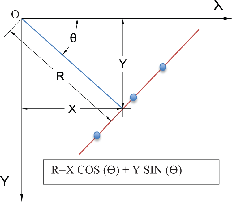
Figure 4: The relation between the coordinates (X, Y) of any point (blue circles) on the shown straight line (red) and the length (R) and the angle θ of the perpendicular line (blue) from the origin (O) to the straight line

Since the LP objects represented in a certain chromosome should have similarities in their widths (W) and heights (H), the MA operator should maximize these similarities by considering the deviation of each gene property from the mean value of the same property in the current chromosome. Hence, the proposed algorithm is composed of three steps as follows:

INPUT: chromosome chrm having L genes with indices j from 1 to L and their corresponding objects (obj = chrm (j)) with location and dimension parameters Xj, Yj, Wj, and Hj.

OUTPUT: chromosome chrm with objects having better collinear and dimension characteristics.

First step: Detect the worst fit object obworst (with index jwrst) which has the largest gene distance GeneDist in chrm, which is defined as follows:

GeneDist(jwrst)=max1≤j≤L(10×|R(j)−Ravg|+4×|DX(j)−DXavg|+3×|H(j)−Havg|+|W(j)−Wavg|)(24)

where

R(j)=Xj×COS(θk)+Yj×SIN(θk),(25)

Ravg is the mean value of R, Havg is the mean value of H, and Wavg is the mean value of W in the current chromosome.

DX(j) is the minimum of the X-distance of the object (j) from its left and right neighbors if it is not at one of the two extreme ends of the chromosome. If the object is at the most left (or the most right) of the chromosome, its distance from the right neighbor object (or the left neighbor object) will be used.

Hence the output of this step is the index of the worst gene (jworst) which corresponds to obworst in addition to other distance values that represent the maximum deviation of each property from its mean.

Second step: finding the best fit object not belonging to the current chromosome to replace the worst fit one. This step will not take place unless one of the following conditions is true:

a)Maximum deviation in R: MaxDevR=|Rworst−Ravg|>0.5×Havgb) Maximum deviation in H:MaxDevH=|Hworst−Havg|>0.33×Havgc)Maximum deviation in W: MaxDevW=|Wworst−Wavg|>0.5×Wavg}(26)

If one of the above conditions is true the worst fit object obworst is replaced by a best-fit object obbest by testing all objects in the near set with indices [obworst − 1.5 × L, obworst + 1.5 × L] and selecting the best one (obbest) that has the minimum GeneDist (obbest). The replacement is performed if GeneDist (obbest) is less than GeneDist(obworst).

Third step: If replacement is done in step 2, the new chromosome angle θ is recalculated and the above two steps are repeated for a maximum of 7 iterations, otherwise the algorithm is stopped.

By applying the above algorithm, the chromosome state is moved to a local minimum as in the Hill-climbing algorithm which speeds up the search process significantly. For instance, after testing the plate used in the experiment shown in Fig. 5, a maximum of 6 generations were needed to reach the optimal solution (in case of no skipping). As mentioned in [17], the search space after using subgrouping is approximatley linearly proportional to the number of CCOs, and based on the hybrird binarization techniques and the resloution (720 (Width) × 1160 (Height)) and complexity of the CCPD dataset, the maximum number of CCOs is about 900. In [17], there were two image resolutions (480 × 640 and 240 × 320) having approximatelly a maximum of 330 CCOs and the experimentally selected maximum number of generations was 10. Hence, in the CCPD case, the required maximum number of generations is about 30, but due to the use of the memetic operator we have decreased the maximum number of generations to 15, which significantly reduces the total number of GA iterations and the LP detection time. By assigning 15 for the maximum number of generations, the average number of generations per image when using the memetic operator are dropped to 9.05 instead of 15 in the case of 30 generations without the memetic operator in the case of the CCPD Base evaluation data section (100,000 images).

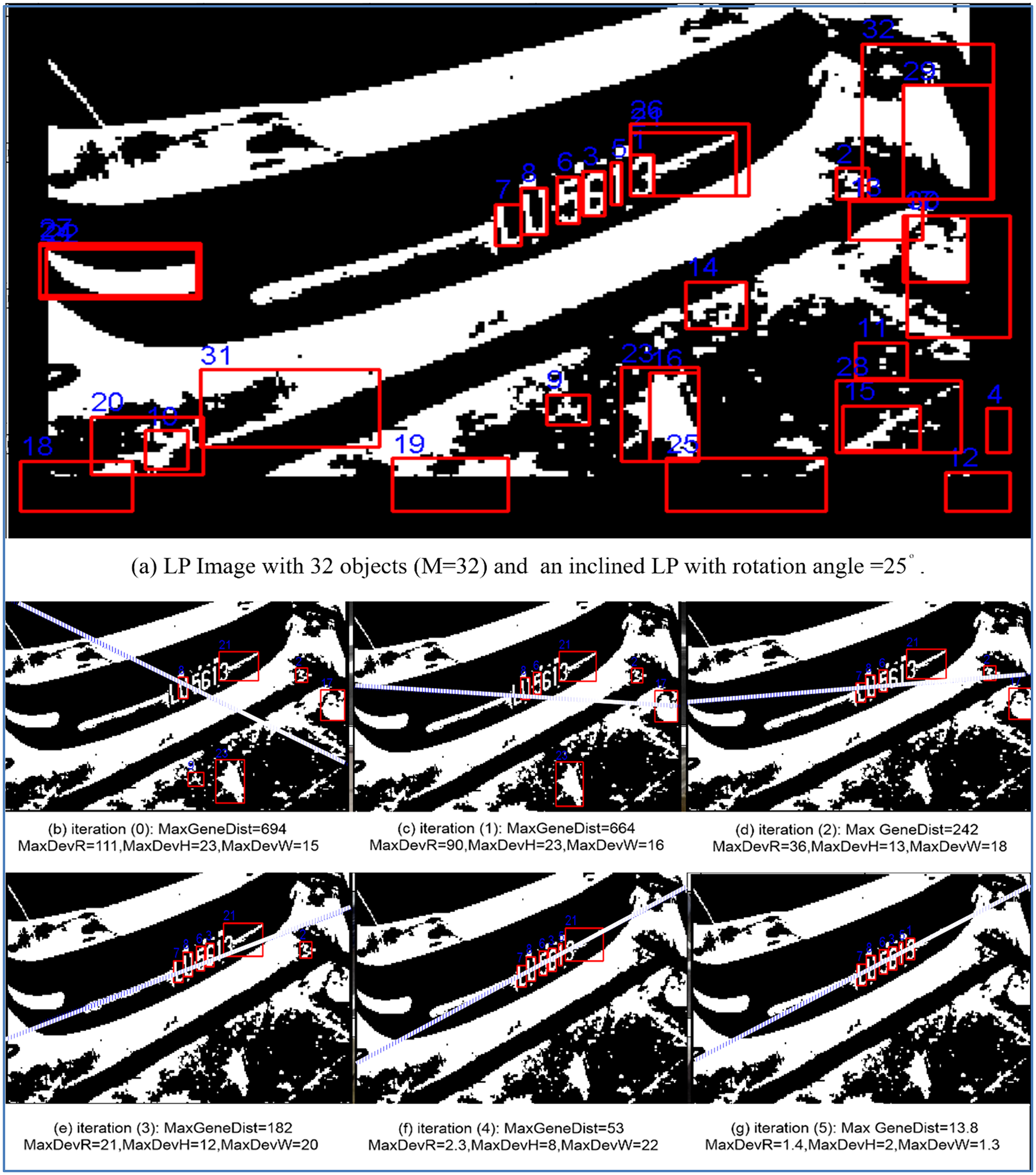
Figure 5: An inclined LP with angle (25°) having all its 6 symbols detected (out of 32 objects) in 5 iterartions where the dashed line indicates the location and orientation of the hough line of the chromosome at each iteration and the red boxes indicate the chromosome objects

It is worth mensionning that the proposed memetic operator mostly allows a partial solution to reach the optimum one even if the partial solution has only 2 out of 6 symbols of the correct (or semi-correct) solution in a given chromosome as in Fig. 5 where an inclined LP with angle (25°) had all its 6 symbols detected (out of 32 objects) in five memetic iterations. The MA iterations are done in every generation of the GA for the best-fit chromosomes only.

Unlike the familiar mutation operator which is executed with a fixed probability not related to the fitness or objective distance of the chromosome, the introduced memetic operator is performed only on the best fit chromosomes whose Objective distances ODs are less than the value (ODmin + ODavg/10) to reduce the processing time and concentrate on the most promising solutions.

Fig. 6 displays an image (part a) from the Rotate section which resulted in 134 CCOs after the objects filtering phase (part b) with two convergence graphs: The first graph (part c) displays the average and the best (objective distance) vs. the generation number without using the memetic operator and the second graph (part d) displays the convergence graphs using the memetic operator. From Fig. 6 the speed of convergence when using the memetic operator is approximately double the speed without using it.

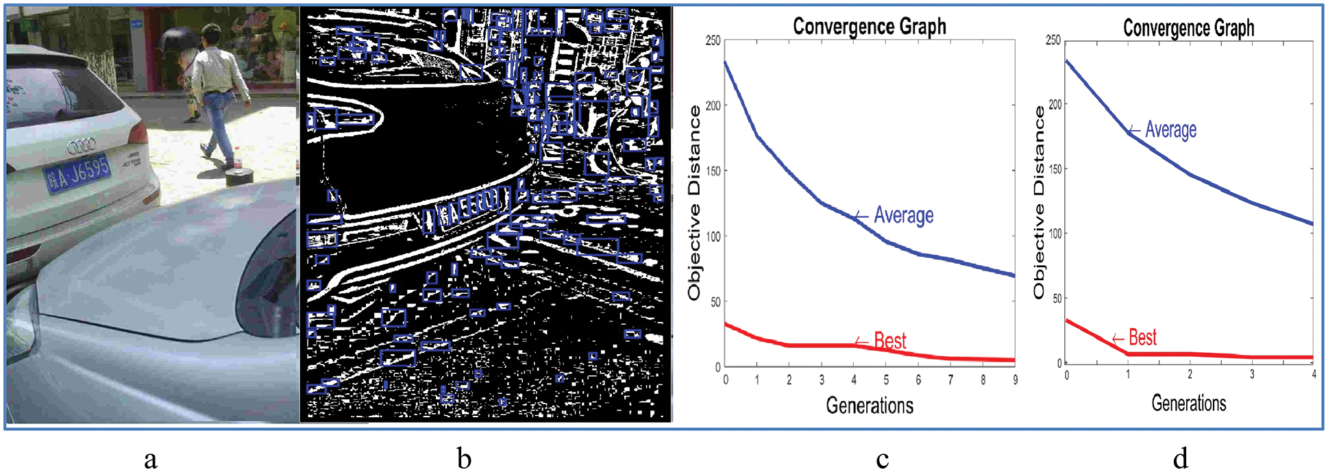
Figure 6: (a) Input RGB image, (b) 134 CCOs in the binarized image, (c) The convergence graphs without using the memetic operator, and (d) the convergence graphs in the case of using the memetic operator

6  Fake Detection Phase

In the previous paper [17], a fake detection stage was introduced using a heuristic function based on the number of the CCOs and the number of black-white crossings in the neighborhood of the detected LP. Because in this research we have a very large training set (100,000 images), we will use a convolutional neural network model to discriminate between LP and non-LP regions. This requires three steps:

1- Generating the training data set

In this step the MA-based algorithm is run on the Base training dataset and for each image the MA-based algorithm is run until an LP is found based on the ground truth data, where the TP regions are stored in the TP folder and the FP ones are stored in the FP folder.

2- Training a ready-made CNN model on the generated training set

In this step we tested two ready-made CNN models, mainly GoogleNet [23] and ResNet18 [24], where higher accuracy results were obtained using GoogleNet. The reason as we guess is that GoogleNet is more sensitive to color-image inputs than ResNet18 because the latter propagates the channel data through addition layers while GoogleNet propagates channel data through depth concatenation layers. Therefore, most of the recent research on the CCPD dataset produce higher accuracy results than previously related deep learning techniques because the color images are submitted to the models without being converted into grey.

3- Optimization of the binary-classification accuracy of the model based on the training data

In this step the enhancement of the produced model is tried in two dimensions. The first dimension regards data augmentation during the training process. In all the conducted experiments, random rotation in the range from −30 to 30 and random shear in both X and Y directions in the range from −10 to 10 are performed. The second dimension regards the contents of the prepared images for the training process. Two cases are tested, in the first case, the training images contain only the regions that just include the LP while in the second case the image area is longitudinally doubled, and the LP region is kept in the center. Fig. 7 presents samples of TP and FP images in the two cases. Based on the flowchart in Fig. 1 and the fact that all the images in the CCPD dataset does not include True Negative (TN) samples, hence the accuracy is measured as TP/(TP + MIS) where MIS means FP or False Negative (FNG). After training the two models in the two cases and testing them on the Rotate dataset section, the accuracy was 88.2% in the first case and increased by 8.2% in the second case reaching 96.2% where the LP context (region around the LP) allowed the CNN model to differentiate between LP and non-LP regions. Unlike most of the previous deap learning techniques that use random regions to represent FP samples, in this research, the FP samples are generated by the proposed technique for cases that have objects sequences similar to the LP symbols (Adversarial samples), which allows the CNN model to concentrate in learning the difference between LP and simi-LP regions and hence performs what we can call “skilled learning” such as skilled and random forgery learning in the case of signature verification.

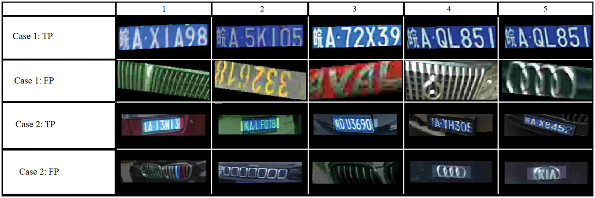
Figure 7: Samples of TPs and FPs training images as generated by the MA-based system in the two cases: same (case 1), and double (case 2) the LP area

A third experiment is conducted based on the second case but after replacing the average global pooling layer in the GoogleNet with a 3 × 3 average pooling layer with a stride 2 × 2 such that the output of the pooling layer is 3 × 3 × 1024 instead of 1 × 1 × 1024. This modification increased the detection accuracy of the Rotate dataset section by 1.6% reaching 97.8% because it allowed the LP context to be well presented to the next fully connected layer and hence higher accuracy is achieved. A further experiment is conducted after increasing the height of the LP area by double the average hight of its symbols (extended by Havg from each side) and the pooling layer is removed such that the input to the fully connected layer is 7 × 7 × 1024. This modification resulted in an increase of 0.90% reaching 98.70% for the Rotate data section. When using the ground truth data for verification instead of the CNN model the accuracy of the Rotate section reached 99.75% which means that the proposed candidates by the MA-based technique cover most of the solution space but because the CNN model is the only data-dependent unit in the proposed technique the accuracy is still less than the maximum allowed limit. Since the technique is based on MA and CNN it will be refered to as MA-CNN Technique.

7  Experiments and Discussion

The evaluation of the MA-CNN technique will be based on the CCPD benchmark dataset [14] and the Aplication Oriented License Plate Data Set (AOLP) [25]. The CCPD dataset has 200,000 images Base section (Train (100,000) and Evaluate (100,000)) plus six special test sections (Rotate, Tilt, Weather, Dark/Bright (DB), Far/Near (FN), and Challenge) which cover most of the complexity dimensions of the LP detection problems. Although CCPD includes a seventh section called Blur it is still not evaluated in the state-of-the-art works. The AOLP contains 2049 images distributed among three application categories (Acces Control (AC), traffic law enforcemnt (LE), and road patrol (RP)). Fig. 8 presents examples of detected samples from the CCPD dataset sections with the rotation angle written under each sample.

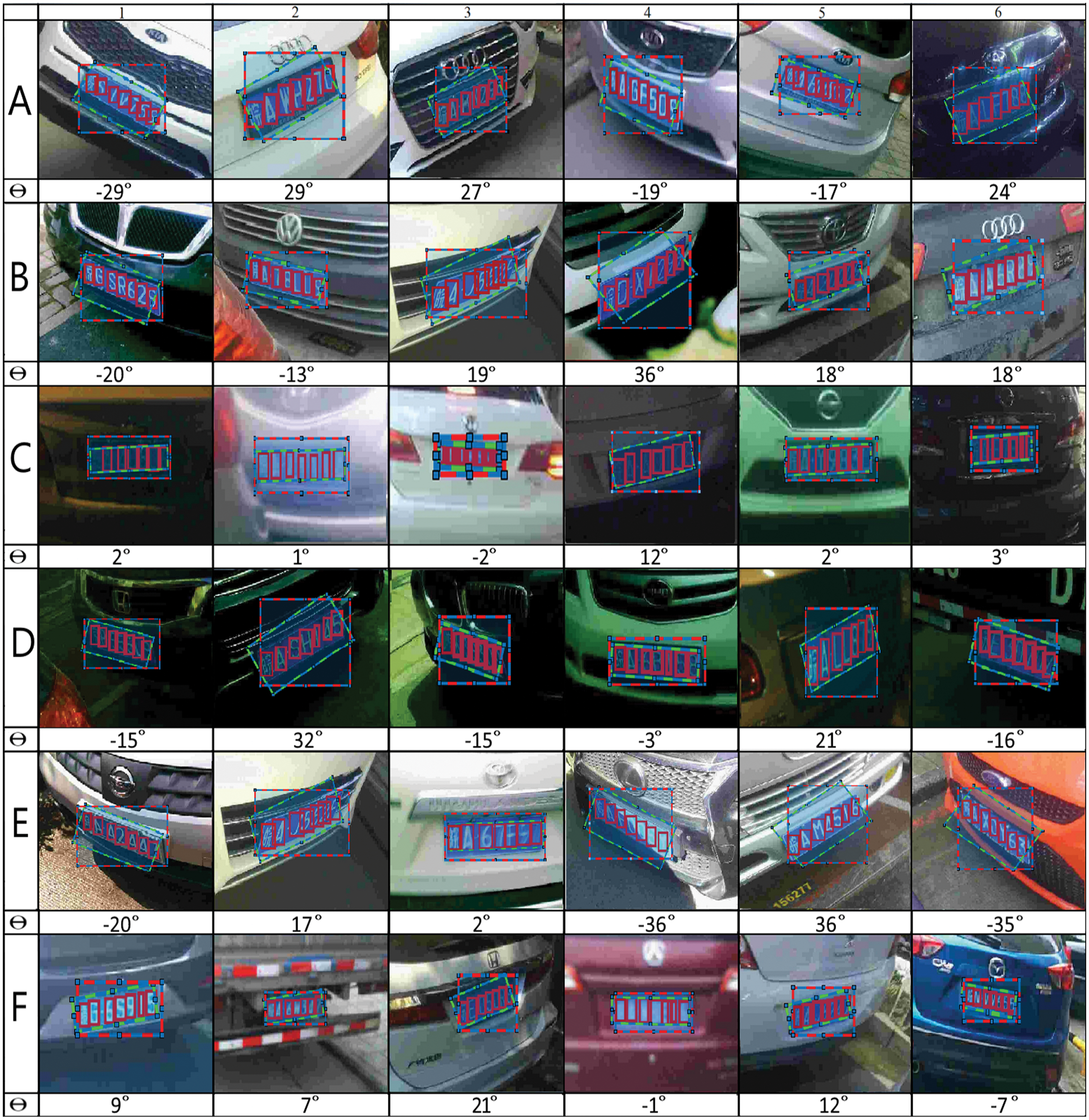
Figure 8: Detected samples from different sections (A: Rotate, B: TILT, C: Blur, D: DB, E: FN, and F: Challenge). Ground truth boxes have red dashes and detected boxes have green dashes

As in [14], a plate is considered detected if the intersection over union (IoU) value is larger or equal to 0.7. The evaluation experiment will be performed on all the CCPD sections based on the precision as it is used in the state of the art papers and defined as follows:

Precision=TP/(TP+FP)(27)

Experiments on the AOLP will consider recall also, which is defined as follows:

Recall=TP/(TP+FN)(28)

All the experiments performed in this research are implemented using MATLAB 19B on a PC with 32 GB random-access memory (RAM), Intel core i7-8700K CPU@3.70 GHz, and a graphical accelerated processing unit (GPU) of NVIDIA GeForce GTX 1080 Ti with 11 GB RAM. Since in [14], the technique output is either FP or TP because the dataset collection application guaranteed the existence of an LP in all samples, the LP miss branch in the flowchart in Fig. 1 is redirected to the accepted LP symbol block to have the same experimental conditions in the case of the CCPD dataset.

Tab. 1 presents the precision results for the seven sections and the average precision (AP) for all sections in addition to the detection speed in frames per second (FPS). The results of the works [10–14] have been recorded as in [14]. In addition to the recorded results in [14], a recent work [26] on CCPD has achieved the highest precision based on an End-To-End deep learning architecture that included two faster-R-CNN subnetworks to detect both LP and non-LP text and used a loss function to prevent the detection of non-LP regions.

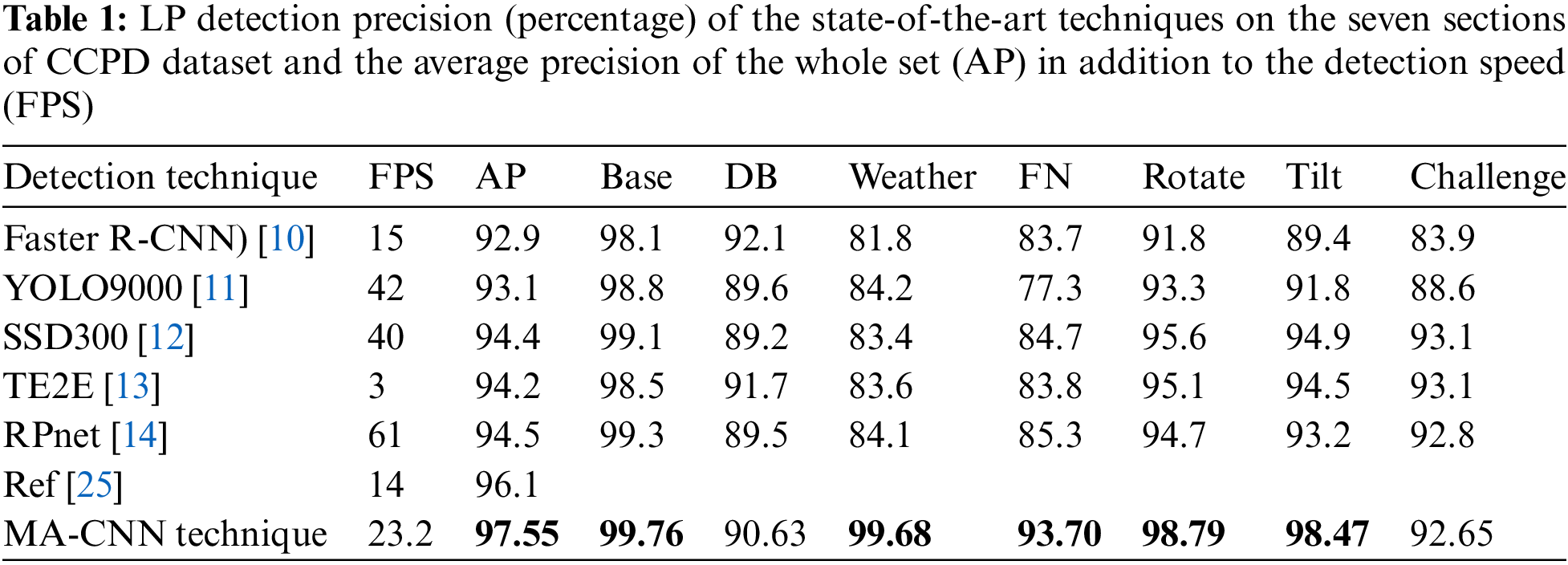
From Tab. 1, it is apparent that the proposed MA-CNN technique outperforms the state-of-the-art techniques in all sections except the DB and Challenge sections. The best precisions (Bold) are for the Base, Weather, Rotate and Tilt sections because the core of the technique is rotation invariant in addition to the rotation and shear augmentations performed during the training of the CNN model. Increasing the precision in the DB, FN, and Challenge sections can be achieved by optimizing the binarization filters and/or adding other techniques given that the system speed is maintained high. Also, other data augmentation related to illumination complexities is needed to increase the accuracy of the CNN model because the BASE training set does not cover all the complexities included in the mentioned test sections.

To adapt the technique parameters for the AOLP dataset, the blue channel is considered with an equal weight to other channels in Eq. (1) and the binarization filter sizes are multiplied by a factor of (ImageWidth/720). The minimum symbol hight (MinH) is set to 11 pixels to allow detection of very small symbols and overcome the main difficluty of the AOLP dataset. The same GRM matrix is used with 6 symbols instead of 7 by execluding the Chineeze character. Since, the color and layout of the AOLP dataset is different from that of the CCPD dataset, in each of the three experiments, the CNN model is retrained on two of the three data subsections and tested on the remaining one to allow verification of the MA-output. Tab. 2 presents the results in case of the AOLP data set categories showing the work of my previous paper [17], the author of the dataset [25] and the recent work of [26].

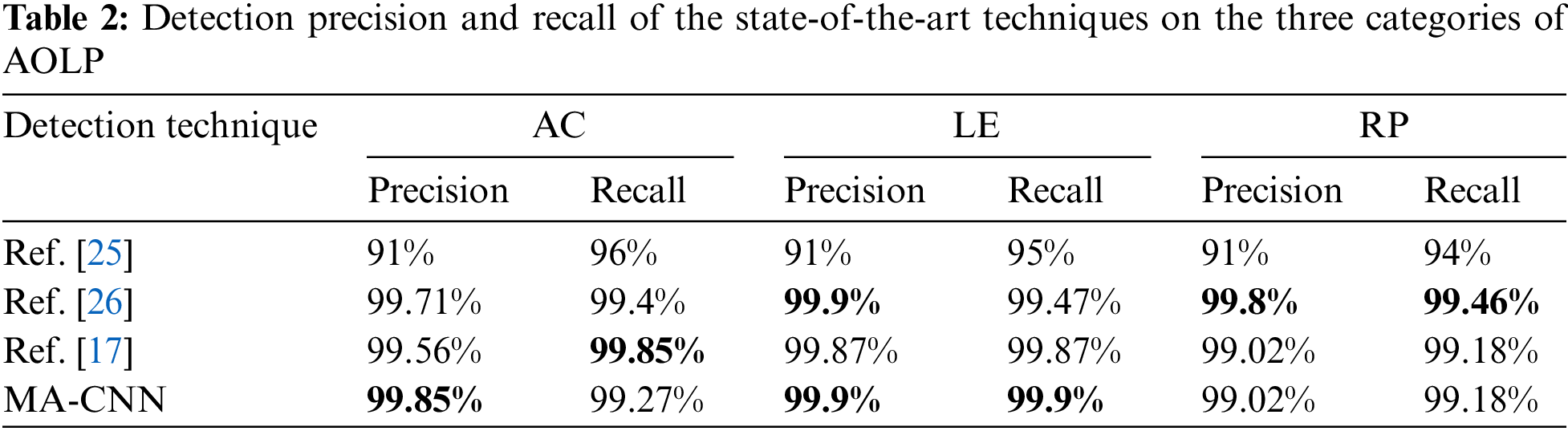
Based on the results in Tab. 2, we conclude that the MA-CNN technique is competing with the [17,26] techniques where the best results (Bold) are alternating between the three techniques. Based on the AOLP experiment, the significant difference between the MA-CNN technique and [17] is the very high speed (120 FPS) compared to 16.6 FPS (for [17]) in the case of low resolution (320 × 240) and 92 FPS compared to 8.3 FPS in the case of the higher resolution (640 × 480).

Although the MA-CNN has been accelerated using C++ and GPU computing in about 50% of the implemented routines, it is still relatively slow compared to the state-of-the-art real-time techniques. This can be overcome by re-implementing all the routines in the memetic algorithm using GPUs.

8  Conclusion

A novel MA-CNN technique has been introduced for the localization of the LP symbols using a memetic algorithm that proposes a candidate solution that is verified by a CNN model which filters out FP solutions and pushes the technique to do more searches for the best solution.

A significant enhancement of the previously designed GA-based system for localizing the vehicle plate number inside plane images has been introduced to support fast and accurate detection of LPs in complex contexts. Hence, a deeper solution to the binarization problems has been introduced to overcome difficult illumination and physical problems. In the binarization stage, a hybrid local adaptive technique with different window sizes and binarization parameters has been introduced to enrich the solution space and to guarantee the detection of the TP solutions if they exist in different perspective and illumination contexts. A neighbourhoud-based filtering stage has been introduced to minimize the number of non-LP symbols and hence minimize the MA search space to support fast and accurate detection of the LP symbols. The output of the connected component analysis stage is enriched by storing the positions and dimensions of every CCA object at any angle to allow accurate calculation of the objective distance between the chromosome genes and the concerned LP GRM defined in one horizontal direction resulting in more accurate and fast localization of the unknown plate. The fake stage in the previous versions has been replaced with a CNN model that is optimized to differentiate between LP and non-LP regions based on the surrounding context of the localized plate. A novel memetic operator has been introduced based on the Hough line representation to perform a local search for the linearly aligned LP-symbols which significantly minimized the search time and guaranteed convergence to the global minimum with the least number of iterations.

Finally, the new MA-CNN technique has been tested on two challenging benchmark datasets, which resulted in highly accurate detection of the LP with a low FP rate. The precision of the new system now competes with the state of the art techniques although maintaining a wider range of angle and scale. The wide range of the complexities of the LP images in the experimented datasets proves the robustness of the new system and its high ability to overcome challenging contexts.

Acknowledgement: The author wishes to thank all the FCIT members, especially the Dean and the Head of the CIS department for the facilities provided to complete this research.

Funding Statement: The author received no specific funding for this study.

Conflicts of Interest: The author declares that he has no conflicts of interest to report regarding the present study.

References

1. J. Shashirangana, H. Padmasiri, D. Meedeniya and C. Perera, “Automated license plate recognition: A survey on methods and techniques,” IEEE Access, vol. 9, pp. 11203–11225, 2020. [Google Scholar]
2. W. Jia, H. Zhang, X. He and Q. Wu, “Gaussian weighted histogram intersection for license plate classification,” in Proc. IEEE Int. Conf. on Pattern Recognition, Hong Kong, China, vol. 3, pp. 574–577, 2006. [Google Scholar]
3. S. Yohimori, Y. Mitsukura, M. Fukumi, N. Akamatsu and N. Pedrycz, “License plate detection system by using threshold function and improved template matching method,” in Proc. IEEE North American Fuzzy Information Processing Society, Banff, Alberta, Canada, vol. 1, pp. 357–362, 2004. [Google Scholar]
4. L. Luo, H. Sun, W. Zhou and L. Luo, “An efficient method of license plate location,” in Proc. 1st Int. Conf. IEEE Information Science and Engineering, Nanjing, Jiangsu, China, pp. 770–773, 2009. [Google Scholar]
5. A. M. Al-Ghaili, S. Mashohor, A. Ismail and A. R. Ramli, “A new vertical edge detection algorithm and its application,” in Proc. IEEE Int. Conf. on Computer Engineering & Systems (ICCES), Cairo, Egypt, pp. 204–209, 2008. [Google Scholar]
6. R. Zunino and S. Rovetta, “Vector quantization for license-plate location and image coding,” IEEE Transactions on Industrial Electronics, vol. 47, no. 1, pp. 159–167, 2000. [Google Scholar]
7. H. Caner, H. S. Gecim and A. Z. Alkar, “Efficient embedded neural-network-based license plate recognition system,” IEEE Transactions on Vehicular Technology, vol. 57, no. 5, pp. 2675–2683, 2008. [Google Scholar]
8. J. Matas and K. Zimmermann, “Unconstrained license plate and text localization and recognition,” in Proc. IEEE Transactions on Intelligent Transportation Systems, Vienna, Austria, pp. 225–230, 2005. [Google Scholar]
9. S. Draghici, “A neural network based artificial vision system for license plate recognition,” International Journal of Neural Systems, vol. 8, no. 1, pp. 113–126, 1997. [Google Scholar]
10. S. Ren, K. He, R. Girshick and J. Sun, “Faster R-CNN: Towards real-time object detection with region proposal networks,” IEEE Transactions on Pattern Analysis and Machine Intelligence, vol. 39, no. 6, pp. 1137–1149, 2016. [Google Scholar]
11. J. Redmon and A. Farhadi, “YOLO9000: Better, faster, stronger,” in Proc. IEEE Conf. on Computer Vision and Pattern Recognition, Honolulu, HI, USA, pp. 7263–7271, 2017. [Google Scholar]
12. W. Liu, D. Anguelov, D. Erhan, C. Szegedy, S. Reed et al., “Ssd: Single shot multibox detector,” in Proc. Springer European Conf. on Computer Vision, Amsterdam, The Netherlands, pp. 21–37, 2016. [Google Scholar]
13. H. Li, P. Wang and C. Shen, “Towards end-to-end car license plates detection and recognition with deep neural networks,” IEEE Transactions on Intelligent Transportation Systems, vol. 20, no. 3, pp. 1126–1136, 2018. [Google Scholar]
14. Z. Xu, W. Yang, A. Meng, N. Lu, H. Huang et al., “Towards end-to-end license plate detection and recognition: A large dataset and baseline,” in Proc. the European Conf. on Computer Vision (ECCV) Workshops, Munich, Germany, pp. 255–271, 2018. [Google Scholar]
15. G. Abo Samra and F. Khalefah, “Localization of license plate number using dynamic image processing techniques and genetic algorithms,” IEEE Transactions on Evolutionary Computation, vol. 18, no. 2, pp. 244–257, 2014. [Google Scholar]
16. G. Abo Samra, “Genetic algorithms based orientation and scale invariant localization of vehicle plate number,” International Journal of Scientific & Engineering Research, vol. 7, no. 4, pp. 817–829, 2016. [Google Scholar]
17. G. E. Abo-Samra, “Application independent localisation of vehicle plate number using multi window-size binarisation and semi-hybrid genetic algorithm,” The Journal of Engineering, vol. 2018, no. 2, pp. 104–116, 2018. [Google Scholar]
18. K. Saddami, K. Munadi, S. Muchallil and F. Arnia, “Improved thresholding method for enhancing jawi binarization performance,” in Proc. Int. Conf. on Document Analysis and Recognition, Kyoto, Japan, vol. 1, pp. 1108–1113, 2017. [Google Scholar]
19. M. H. Najafi, A. Murali, D. J. Lilja and J. Sartori, “GPU-accelerated nick local image thresholding algorithm,” in Proc. IEEE Int. Conf. on Parallel and Distributed Systems, Melbourne, Australia, pp. 576–584, 2015. [Google Scholar]
20. T. R. Singh, S. Roy, O. I. Singh, T. Sinam and K. M. Singh, “A new local adaptive thresholding technique in binarization,” International Journal of Computer Science Issues, vol. 8, no. 6, pp. 271–277, 2011. [Google Scholar]
21. C. Cotta, L. Mathieson and P. Moscato, “Memetic algorithms,” in Handbook of Heuristics, Cham: Springer, pp. 607–638, 2018. [Google Scholar]
22. K. Zhao, Q. Han, C. -B. Zhang, J. Xu and M. M. Cheng, “Deep hough transform for semantic line detection,” IEEE Transactions on Pattern Analysis and Machine Intelligence, vol. 44, no. 9, pp. 4793–4806, 2022. [Google Scholar]
23. C. Szegedy, W. Liu, Y. Jia, P. Sermanet, S. Reed et al., “Going deeper with convolutions,” in Proc. IEEE Conf. on Computer Vision and Pattern Recognition, Boston, MA, USA, pp. 1–9, 2015. [Google Scholar]
24. K. He, X. Zhang, S. Ren and J. Sun, “Deep residual learning for image recognition,” in Proc. IEEE Conf. on Computer Vision and Pattern Recognition, Las Vegas, NV, USA, pp. 770–778, 2016. [Google Scholar]
25. G. S. Hsu, J. C. Chen and Y. Z. Chung, “Application-oriented license plate recognition,” IEEE Transaction on Vehicular Technology, vol. 62, no. 2, pp. 552–561, 2013. [Google Scholar]
26. Y. Lee, J. Jihyo, Y. Ko, M. Jeon and W. Pedrycz, “License plate detection via information maximization,” IEEE Transactions on Intelligent Transportation Systems, pp. 1–14, 2021. https://doi.org/10.1109/TITS.2021.3135015. [Google Scholar]
Cite This Article
Copyright © 2023 The Author(s). Published by Tech Science Press.
This work is licensed under a Creative Commons Attribution 4.0 International License , which permits unrestricted use, distribution, and reproduction in any medium, provided the original work is properly cited.
Downloads
Citation Tools