Gait Image Classification Using Deep Learning Models for Medical Diagnosis

1  Introduction

1.1 Walking Gait

Gait is a medical term for the way a person walks. “Walking gait” refers to the rhythm that a leg goes through in one step of walking. Gait analysis essentially studies movement, particularly human perambulation. It visually assesses a person’s gait to measure body movements, muscle activity, and the mechanics of the body. It uses a person’s stride to visually evaluate their body mechanics, muscle activation, and movement patterns. This is mostly used in the realm of medicine to assess and examine a person’s gait in order to diagnose and cure any abnormal diseases that may be brought on by it.

Since innovations in medical and clinical image processing have been more prominent, gait analysis has become more prevalent. Gait analysis has not only contributed to finding abnormalities in a user’s walking pattern, but also in disciplines such as user identification in biometrics, influence investigation, sports where the gaits of athletes are examined, and for the elderly, who can be constantly monitored and identify if they are going to fall.

All methods of biometric recognition in existence, such as Iris, fingerprint, voice, and facial recognition, require an individual’s cooperation in order to perform biometric validation. However, biometrics using gait analysis gives a huge advantage since an individual’s direct contact is not required to verify their biometrics. Their biometrics can be analyzed even from a larger distance using a Closed-Circuit Television (CCTV) camera. This can be implemented in various applications like airports, train stations, bus stations, clinical analysis, and bank surveillance.

In the field of medicine, the gait of the patient is studied to make a diagnosis of certain diseases. Early detection of gait patterns can aid in the diagnosis of disorders such as cerebral palsy, Parkinson’s disease, and Rett syndrome (RTT). Parkinson’s disease impacts the human body’s postural skills and people with cerebral palsy experience passive movement of limbs and difficulty with muscle control [1] due to a condition known as spasticity, which disrupts a normal gait. Gait abnormalities are also brought on by RTT, a neurodevelopmental disorder [2]. Gait analysis, therefore, functions as a tool for health indicators.

1.2 Recording Gait Data

To record gait data, many detecting modalities, such as wearable sensors attached to the human body, such as accelerometers, gyroscopes, power, and tension sensors, can be utilized. Non-wearable gait frameworks, however, capture step data using imaging sensors without the involvement of the subjects and even from a great distance away. The goal of this research is to provide a better solution to classifying vision-based walk recognition frameworks that have traditionally relied on profound learning.

The exhibition of vision-based gait recognition frameworks, henceforth simply alluded to as step acknowledgment, can be impacted by i) variations in the appearance of the individual, such as carrying a purse/bag or wearing things of attire like a cap or a coat; ii) variations in the camera perspective;iii) hindrance factors, like areas of the subject’s body being partially or completely hidden by an item or a limb. It is important to look through all these acceptances while evaluating vision-based gait analysis.

1.3 Classifying Gait Data

To distinguish human gait, a number of computer vision and machine learning methods are applied. They can be Model-based or model-free approaches. A model-based technique is utilized to examine gait patterns using human anatomy. It can include elements such as the angle between the joints, the ankle, and so on. This method can be utilized when the principal factor affecting the subject’s performance is the type of clothing worn, the presence of a bag, or a change in angle. This method has a high computational cost, yet it is effective with high-level data.

The alternative technique, model-free, works best with human body silhouette data. This strategy is more responsive to various aspects such as changing circumstances, shadow impact, and different clothing. This technique is more cost-effective and faster. As a result, finding a middle ground between these two approaches is critical for the model to be both fast and accurate, making human gait analysis a significant research topic.

Generally, in a human gait recognition system, the input data is a video or a sequence of image frames of a person walking. Images, in general, have a lot of noise, low resolution, complex backgrounds, and so on. Hence, it is important to extract all these images precisely in order to get the proper gait analysis. The better the image, the better the model can train and give an accurate analysis.

In this research, the dataset used, provided by the Chinese Academy of Sciences (CASIA), contains image frames of silhouettes of human gait. All gait images in the dataset are classified under five categories: normal walk, fast walk, slow walk, and walking wearing a coat or a bag. Moreover, it is difficult for a human to distinguish through the naked eye if a person’s gait is normal or abnormal, thereby making the task of evaluating a person’s walking pattern in terms of biometrics or diagnosing a person’s disorder impossible.

Hence, it is important for the concept of deep learning to come into play. The Artificial Neural Network (ANN) based Deep learning models perform better than the usual machine learning models in terms of image analysis. Through numerous stages of processing, it pulls progressively higher-level information from input.

1.4 Research Contributions

This research proposes the use of deep learning techniques such as CNN (Convolutional Neural Network) and CNN-LSTM (Long Short-Term Memory Network) to classify human gait data.

To compare the results obtained by the proposed models, six transfer learning models are incorporated. They are MobileNetV2, InceptionV3, Visual Geometry Group (VGG) such as VGG16, VGG19, Residual Networks (ResNet) like ResNet9, and ResNet50.

The CASIA B and CASIA C datasets were combined according to their classes. For the purposes of uniformity, all the models are trained on a fraction of the combination.

Moreover, multiple types of comparisons are done to find the most efficient parameter for the best classifying model.

2  Related Works

The state of the art in gait classification using image data and the use of the CASIA Gait Database was explored. However, novel gait classifiers were observed to use data from a variety of sensors for classification.

The study by [3] aims to improve the performance of deep learning models in the field of human gait analysis. The feature selection has been highlighted as an attempt to improve the already limited accuracy provided by CNN models. To avoid losing any features, an aggregation of VGG16 and AlexNet features were utilized. Together with the same, the Kernel Extreme Learning Machine (KELM) gets the best recognition accuracy for CASIA datasets A and B. Though the accuracy grew, so did the execution time. An increase in accuracy of 96.50% and 96.90% on CASIA B’s 54° and 90° data proved to be a significant improvement over the prior system.

Gait analysis and monitoring are critical in the prediction of age-related and neural network-based issues in the human body. Wearables like the ones created by [4] in this study can record and analyze gait in real-time. The inertial sensor-based wearable was tested using a self-recorded dataset. This research also suggests a novel gait metric based on Eigen analysis that can distinguish across gaits, demonstrating its potential as a diagnostic tool.

Using gait as a biometric has a significant advantage because it can identify the subject from a distance. The system [5] seeks to create a system that can accomplish the same. The parameters considered are the movement of the leg and stride length. Walk pattern data collection is done using Inertial Measurement Unit (IMU) sensors on cell phones and an Arduino’s resistive flex sensor. To recognize the subject, several classifiers such as tree classifiers, rule-based classifiers, Support Vector Machines (SVM), K Nearest Neighbours (KNN), and Naive Bayes were used. The models were trained using data from a diverse set of people.

The DeepSole is yet another portable device that captures the wearer’s gait. This technology created by [6] characterizes the wearer’s gait and gives vibratory feedback to the user. The design incorporates three neural network models: the first, a Recurrent Neural Network (RNN) that classifies gait, the second, an encoder-decoder RNN that maps sensor data to the actual value, and the third, an Exponentially Delayed Fully Connected Neural Network (ED-FNN) that detects gait freezing. The model’s precision was calculated and found to be in the middle of all subjects. The model was accurate for 83% of the stride cycle. These algorithms can be expanded to distinguish circumstantial events in diseases, as well as retrain stride irregularities like imbalance and muscular weakness, and biometric sensor security.

The gait analysis laboratory at Newington Children’s Hospital (NCH) used a video-based data collection technique. The methodology suggested by [7] uses the gait image to identify the angle, orientation, and center placement of joints. This model was developed at NCH in 1981 based on the radiographic evaluation of 25 hip investigations. In the hip joint and pelvic regions, this model achieved an R-square coefficient of 90%.

The proposed methods necessitate a wide range of images to estimate posture skeletons, which negates the benefit of most datasets because they only provide silhouettes. As a result, [8] conducted tests on two publicly accessible datasets that provide Red, Green, and Blue (RGB) images, the CASIA Dataset A and the CASIA Dataset B. The proposed approach focuses on gait analysis in light of posture. Two stride recognition methodologies “PoseDist” and “PoseFrame” were suggested. Tests were run on all perspectives on the CASIA Datasets A and B, and the continued technique produced best-in-class results, with “PoseDist” achieving an exactness of 98.75% on horizontal, angled, and opposite views, respectively, and “PoseFrame” achieving a precision of 97.5%.

A study using three angles (0, 18 and 180) of the CASIA B dataset was presented in [9]. The data is normalized before being fed into two pre-trained models: ResNet101 and InceptionV3. To optimize the retrieved characteristics, completely automated deep learning and Improved Ant Colony Optimization (IACO) were applied. The accuracy obtained for angles 0, 18, and 180 after final classification using cubic SVM is 95.2%, 93.9%, and 98.25%, respectively.

This research by [10] presents smart footwear that assists the elderly by detecting their walking behavior. 20 types of sensors, including 16 piezoelectric sensors to measure pressure, 3 accelerometers, one for each axis, and one temperature sensor, are used to measure the required parameters to estimate gait and send warnings about risks in the near future. This alert is sent to the caretaker via the Maturo Application. Layered ANNs and multi-layer perceptrons prove to be efficient with an accuracy of 84.0%.

An intelligent system that utilizes pressure plates to measure the pressure exerted during walking, processes the data and sends it to any smart device [11]. The system’s execution necessitates the use of a pressure plate-containing special insole put in the footwear. The weight, number of steps completed, Body mass index (BMI), and number of calories burned are among the data processed and inferred. Patients undergoing rehabilitation can use the system as a support tool and gain analytical insight.

This study by [12] uses data collected from inertial sensors embedded in smartphones. Because smartphones are widely utilized by the common person, data collection is practical, unrestricted, and affordable. To learn and model the data relating to the gait of the user, CNN and RNN are used to abstract the features that are then represented by a hybrid Deep Neural Network. Using the smartphone sensors, distinct datasets are obtained for identification and authentication. The users’ recognition and verification accuracy rates were 93.5% and 93.7%, respectively.

A review of the state of the art in gait analysis of deep learning models was discussed by [13]. The modalities for catching the stride information are categorized by the detecting innovation: video, different sensors like wearables and floors, and public datasets. Established ANNs are compared for each category. Among these, LSTM networks are great for taking care of time-sequential data where solicitation is of importance, similar to step data groupings. Deep learning CNNs outperformed all models and yielded a precision of 95% in tests with 42 patients classifying gait as quick, ordinary, or slow. LTSM accomplished an accuracy of 91.3% on stride classification. Learning from Multi-sensor, multi-modality gait information opens opportunities for robust biometrics and personal healthcare.

The gait data acquired from the open-source data set Human Gait Database (HugaDB) is used in the study [14] which includes a variety of actions such as running, strolling, standing, and sitting. Six wearable inertial sensors on the right and left thighs, shins, and feet were used to collect data. In addition, two Electromyography (EMG) sensors were used on the quadriceps to measure muscle activity. A total of 18 people were used to collect 2,111,962 data. The proposed system used the IB1, a basic instance-based learner, Random Forest, and Bayesian Net algorithms to reach an accuracy of above 99%. The system can be used to identify individuals in crowded areas.

The Support Vector Regression models can be used to acquire gait parameters such as the velocity of walking, stride length, foot clearance, etc., [15]. This was collected with the help of Sport sole, a custom-made insole that can be used in any shoe. This paper proposes an original 2-venture alignment strategy to extricate exact assessments of essential step-to-walk stride boundaries from specially designed instrumented insoles through relapse models during walking and running tasks. Gait metrics were extracted from around 14 healthy people during walking and running. The accuracy of the proposed model is nearly 85%, and it is observed that machine learning regression provides a new approach for improving the accuracy of wearables.

Also, make use of wearable sensors such as gyroscopes and accelerometers to collect gait information of the wearers [16]. Artificial Intelligence techniques were applied to track down examples and specific qualities for every client. Gait recognition is done using a deep RNN model with LSTM and dense layers. Prediction of gait into any one of the predefined 6 categories yields an accuracy of 97% in most executions. The outcomes likewise show a slight improvement in results when utilizing both the speed increase and the gyrator sensors together, albeit the intricacy of the calculation.

Person Recognition based on Gait Model, (PRGM) involves identifying individuals based on their gait, [17] proposes a CNN model with augmentation of data. The model was evaluated using Market dataset-image gait data of different individuals obtained during the CoronaVirus Disease (COVID-19) pandemic. The aim of the paper was to identify people wandering out during the spread of COVID, in the absence of another biometric. It is observed that the accuracy of the CNN model increased from 82.0% to 96.23% after augmenting the data.

The study by [18] illustrates how non-invasive devices can be used to diagnose movement abnormalities without the need to see a doctor. The LSTM algorithm proposed in this paper outperforms the performance of the CNN algorithm. The in-shoe pressure was measured for 12 different people by altering the soles of the shoes. The accuracy of the LSTM model on streaming data for 2 s was 82%. It was demonstrated that intentionally produced gait changes can be categorized using LSTM, demonstrating its efficiency for real-time data.

The classification of different gait patterns using deep learning techniques using the data obtained from intelligent insoles of shoes [19]. The dataset consists of seven categories of gait ranging from running to hill climbing. The ‘FootLogger’ insole was utilized to gather gait information, which is transmitted via Bluetooth to the smartphone of the user. The proposed strategy comprises pre-processing of information and Deep Convolutional Neural Network (DNN) based information extraction. An accuracy as high as 90% was reached. Varying ages were not taken into consideration in this study.

The paper presented by [20] reviews 2 major technological advances in the field of human gait analysis: wearable sensors and machine learning models. Wearables provide a helpful, proficient, and cheap method for gathering information, and Machine Learning Methods (MLMs) aid in gait data retrieval for examination. For the orderly audit and investigation, the Preferred Announcing Items for Systematic Reviews and Meta-Analyses (PRISMA) strategy is utilized. This paper investigates the most recent patterns in step examination utilizing wearable sensors and MLMs. From the outset, an outline of step examination and wearable sensors is introduced. The focus area is on critical step boundaries, wearables, and their materialism in stride examination. When the step boundaries are acquired using Principal Component Analysis (PCA), which eliminates the repetitive stride data, the accuracy of SVM classification is highest. These outcomes are superior to utilizing a 101-layered step design in which PCA isn’t utilized, with an accuracy of 87%.

This study by [21] investigates how gait classification is done using time-frequency analysis of radio-frequency data. According to whether the arms are moving freely or being restrained, the classification is made. The time-frequency representation of the micro-Doppler is used to extract the motion signatures of the arm motion. Hermite’s method is used to calculate the time-frequency, and the authors assert that it accurately depicts the Doppler linked to the human stride. The authors assert that the system performed well in tests using actual radar data.

In this study by [22], ANNs and SVMs are used to analyze a patient’s gait in order to detect motor Parkinson’s disease. The features that are taken into account during the training of the models are the kinetic, kinematic, and spatiotemporal parameters. The use of intra-group and inter-group normalization, two distinct preprocessing techniques, is also explored by the authors. The models’ outputs demonstrate that the intra-group normalized spatiotemporal parameter combination provides excellent performance on both neural networks and SVMs.

This study by [23] suggests a novel method of combining appearance-based and model-based gait recognition techniques. A two-branch neural network, a convolutional neural network trained on the silhouette data, and a graph convolutional network trained on the skeletal data are used to achieve this. To reflect the skeletal data more accurately, the authors also add two new modules to the graph convolutional network. The system learns the spatiotemporal data by first training with the two-branch model and then employing a multi-dimension attention module. The system that was tested using the CASIA B dataset, according to the authors, generates findings that are cutting-edge.

The creation of a system to recognize human gait using a novel model known as “Convolutional Bidirectional Long Short-Term Memory” (Conv-BiLSTM) is discussed in this paper by [24]. An LSTM model is trained on the gait data to learn the temporal information, and ResNet-18 is used to extract the features from the gait data. The deep features are then extracted and given to a You Only Look Once (YOLO) algorithm called the tiny-YOLOv2 model, for prediction using what the authors refer to as a YOLOv2-squeezeNet model. On the CASIA A, B, and C datasets, the authors assert that this dual-phase system delivers up to 90% accuracy. The authors claim that their method outperforms other current research at the time of writing.

After this study, it was observed that the state of the art was not generally performed on the CASIA C dataset. CASIA B was the most broadly adopted dataset for classification, followed by CASIA A. However, gait classification was commonly done using self-recorded data gathered with the use of a variety of sensors.

3  Methodology

Image classification was performed on datasets B [25,26] and C [27] obtained from the CASIA Gait Database. The images from both datasets have been combined into five classes: “normal”, “fast_walk”, “slow_walk”, “with_bag” and “in_coat”. Due to the large number of images impacting training time, a select number of random images were chosen from each class of images.

The OpenCV (Open Source Computer Vision) [28] Python library, version 4.5.5, is used to read the images and extract the pixel data from them. The images are then resized to a standard size of 220 × 220. Feature preprocessing is then performed on the image data by first normalizing the pixel values. The labels are then encoded to enable the deep learning models to train on them. The data is then split into a training and testing set, with 80% of the total data allocated to the training set and the rest to the testing set.

Data augmentation is then performed on the training data. The environment used for conducting this research is Google’s Colaboratory. The system uses the Ubuntu 18.04.5 Long Term Support (LTS) operating system with an Intel Xeon processor and 12986 MiB (MebiByte) of memory. Graphics processing unit (GPU) support was enabled to train the models using the NVIDIA Tesla K80 GPU.

The proposed CNN and CNN-LSTM architectures are compared with transfer learning models that are also trained on the same data, adopting the same flow as seen in Fig. 1. The transfer learning models used in this work are MobileNetV2 [29], VGG16 [30], VGG19 [31], InceptionV3 [31] ResNet50 [32], and ResNet9 [32]. These models are imported using version 2.8.2 of the Python library, Tensorflow. The models are validated with the testing set, and the loss and accuracy across the epochs are visualized.

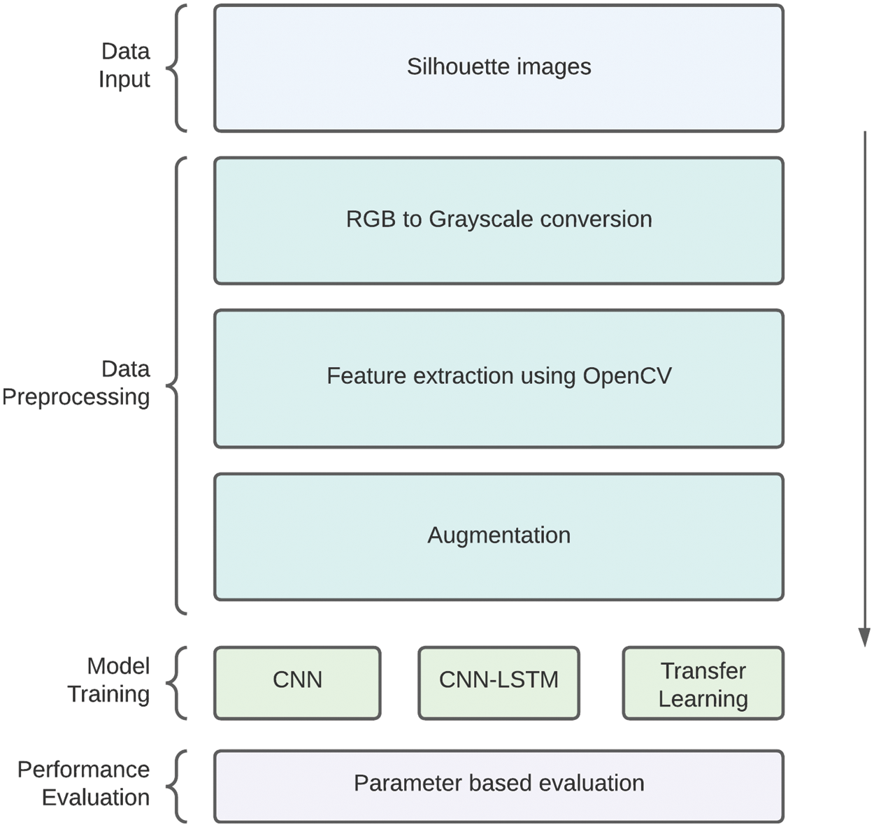
Figure 1: Flow diagram for the study

This research performs a comparison of the performance of the models before and after data augmentation across 250 epochs. Other parameters, such as the number of convolutional layers, dropout layers, and regularization, are varied, and the performance of the proposed models is compared and analyzed across the variations. The best parameters are taken for both the proposed models and they are compared along with the transfer learning models by changing the optimization function. The results of this comparison provide insight into the benefits of using the proposed models over other transfer learning approaches.

3.1 Dataset

By studying how they walk or run, people’s distinctive movements can be identified, normal gait patterns can be defined, and treatments to remedy irregularities causing discomfort can be devised and evaluated. The CASIA Gait Database is provided by the Institute of Automation, Chinese Academy of Sciences for gait recognition, and associated research in order to promote research. This dataset is essentially a set of images containing human silhouettes from video files, and it has 3 parts: A, B (multiview), and C (infrared). The models, both proposed and the ones used for comparison purposes, were trained and evaluated on CASIA B and CASIA C datasets.

Dataset B has 124 people, whose gait was captured from 11 different angles, with 3 categories: normal, with a coat, and with a bag. Dataset C includes the gait of 153 people. It takes into account the following walking conditions, the silhouettes of which were collected by an infrared (thermal) camera: normal, fast walk, slow walk, and with a bag. It was deemed appropriate to integrate both datasets to create a new collection of approximately 96,000 images categorized into five classes. A portion of the dataset consisting of classes: “normal”, “fast_walk”, “slow_walk”, “with_bag” and “in_coat” was taken. All the different deep learning models, including the proposed and transfer learning models, were evaluated using a portion of this newly formed dataset.

As shown in Fig. 2, the dataset with 96,000 images was reduced to a set containing approximately 2273 images across all five classes, which was used to train and evaluate the model. This was done due to the availability of limited resources and computational power.

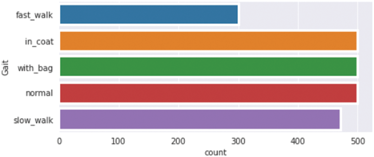
Figure 2: Size of the dataset as per the class labels

Because storing and retrieving such a large amount of data is costly, data augmentation was used on the smaller set of data to improve the performance of the deep learning models under evaluation. The Keras ImageDataGenerator was used to augment in real-time to save overhead memory.

3.2 Preprocessing and Data Analysis

Data preprocessing is a required step that is done prior to training any model because the efficiency and precision of the predictions heavily depend on the quality of the data used. It is an important and necessary step to be performed before analyzing the data. Data analysis refers to the process of cleaning, examining, manipulating, and modeling raw data with the goal of uncovering usable information and acquiring the semantics of the data collected. Ultimately, data analysis helps make informed decisions with the extra knowledge obtained from the examination.

Preprocessing image data may include conversion to grayscale to reduce computational complexity, re-scaling the image data pixels to a predefined range, thereby normalizing their impact, augmenting data to prevent learning of irrelevant data, and standardizing data.

To extract the required and relevant information from the data, feature extraction techniques are used, implemented using OpenCV. The function imread is employed to read all the silhouette images and extract the pixel RGB values of the images. They are resized into a 220 × 220 matrix using the resize function provided by OpenCV. All these matrices are added to a list called “features” and the image target values are read and added to a list called “labels.” After the features have been extracted and placed in the appropriate location, the feature values are standardized by dividing them by 255. The RGB values of the pixels that make up the silhouette image are the feature values.

The features matrix is then reshaped into an order suitable for training the models using Numpy’s reshape function. The labels are encoded and translated from text to integers using the LabelEncoder from Sklearn (scikit-learn) version 1.0.2. The target vector is converted to a binary class matrix using the categorical function from Tensorflow’s Keras API (Application Programming Interface). The training and testing data are split into a 4:1 ratio, with 80% going to training and the remaining 20% going to testing.

In this study, the models are trained on a subset of the datasets, CASIA B and C. The image data in CASIA B focuses on the angle of view of the gait, with the subject wearing either a bag or a coat. CASIA C, however, contains images representing different walking styles, such as normal walking, slow walking, fast walking, and walking with a bag. By combining both datasets, the proposed system observed a total of 5 classes as seen in Fig. 3.

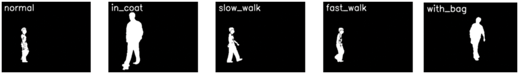
Figure 3: Sample dataset images captured from different angles

After visualizing the data, the images were observed to be of different sizes. The Python library, OpenCV, was used to resize all the images in the dataset to a uniform size of 220 × 220 for all deep learning models, with the exception of 180 × 180 for ResNet models. Fig. 4 represents the resized sample images from the dataset. On merging the CASIA datasets B and C, a set of 96,000 images was obtained. When all the data was used, storage and retrieval became a problem due to the availability of limited resources, so a subset of the dataset was extracted.

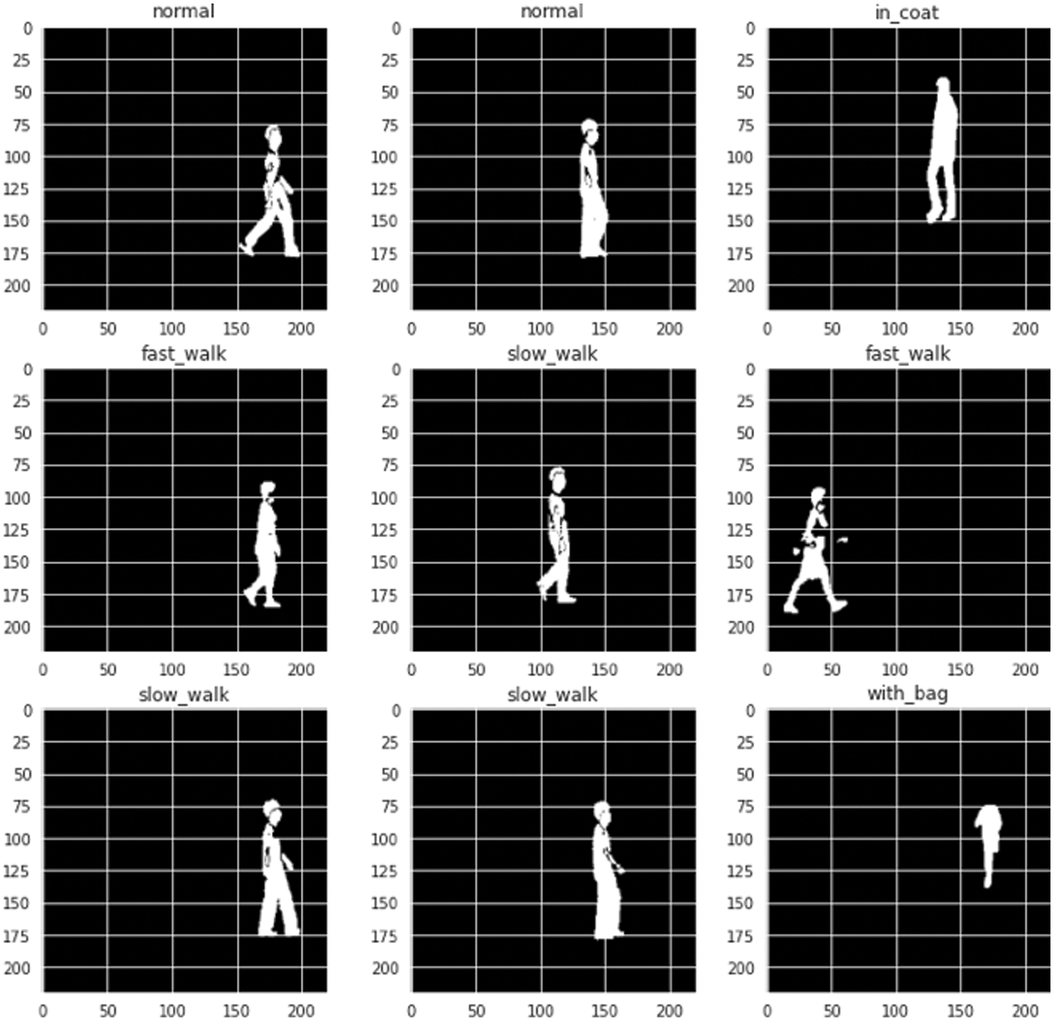
Figure 4: Resized 220 * 220 images from all classes captured from different angles

This was followed by data augmentation. A machine learning model works efficiently when the dataset is rich and sufficient. The accuracy of a model is also dependent on the amount of data it is trained on; the more the data, the more it can learn and the better it can predict. Data augmentation is a set of processes for artificially inflating the amount of data available by producing additional data points of relevance from current data. This entails making minor changes to existing data or applying deep learning models to generate new data of relevance. The ImageDataGenerator offered by the Keras preprocessing module was used for the augmentation. The images in the dataset have been reasonably flipped, rotated, expanded, and transformed.

The transformed images obtained in a batch are visualized using the make_grid method from torchvision. A different batch of images is produced every time the code is run. This can be viewed in Fig. 5. Fig. 6 shows the augmented data which has been rotated, expanded, and randomly transformed. It was observed that the accuracy of most models including the proposed CNN increased by 10% to 15%.

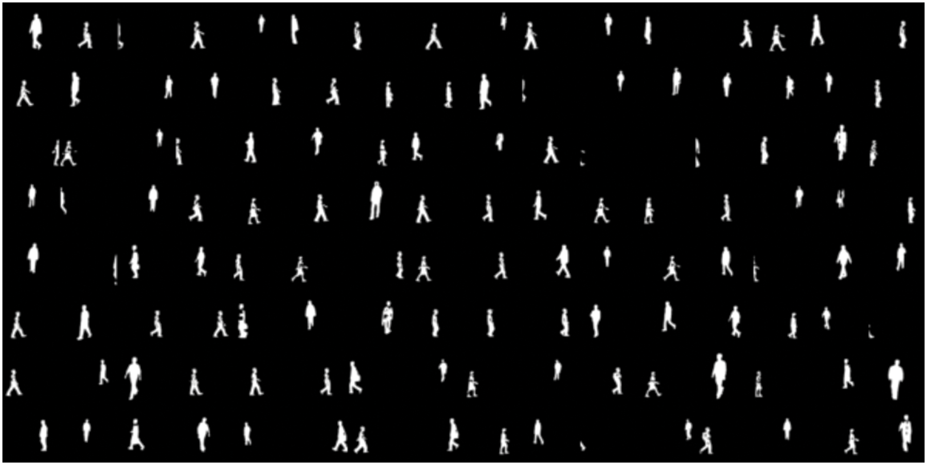
Figure 5: All the merged images as per the batch size visualized

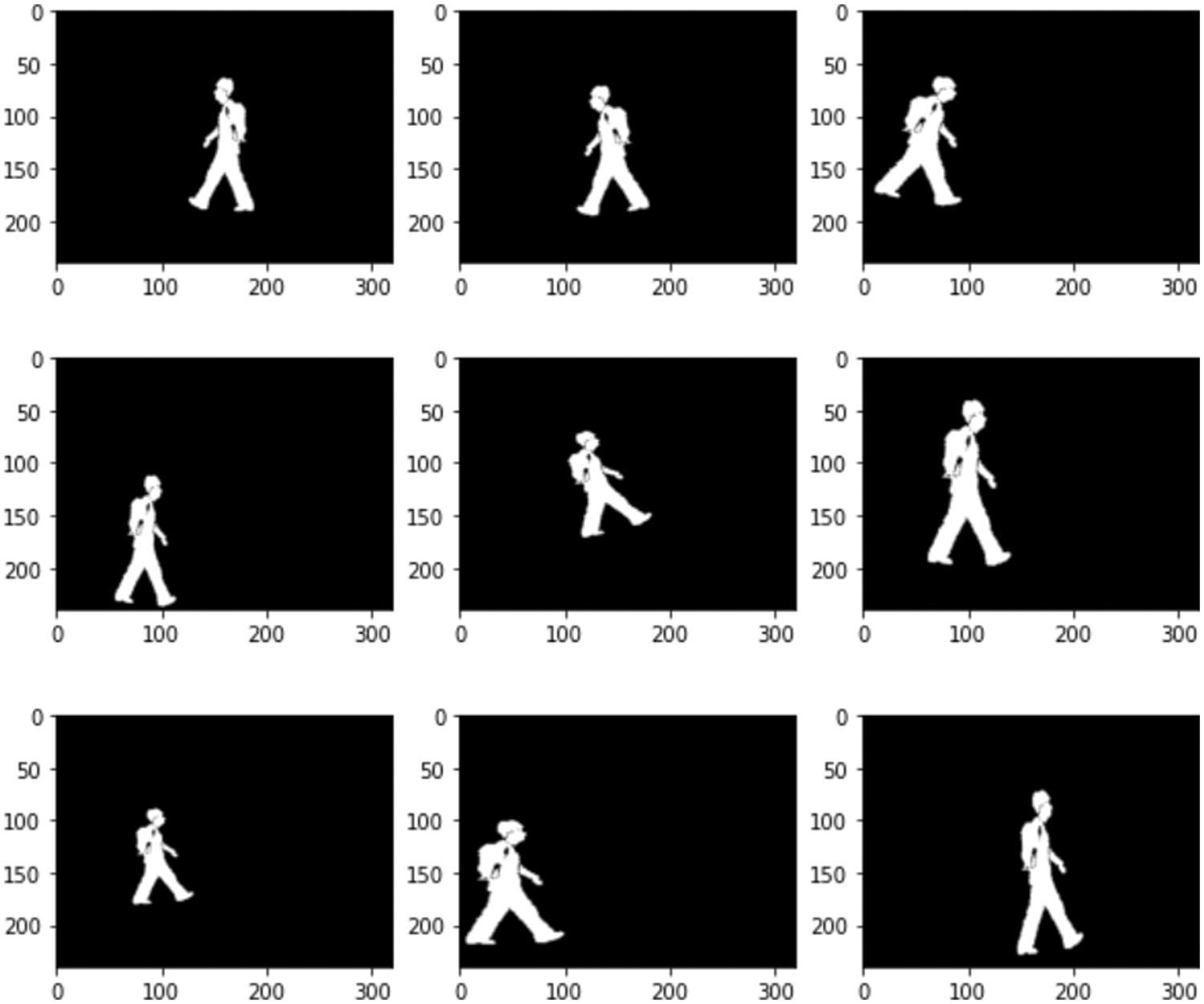
Figure 6: Insights of the slow_walk class after data augmentation

3.3 Proposed Models

3.3.1 Convolutional Neural Networks (CNNs)

All CNNs consist of two parts, the first part consists of convolutional layers that extract the edge and pattern features from the image, and the second part consists of an ANN that trains on the extracted features. The CNN models solely focus on image data and are widely used for classification, object detection, and segmentation tasks. The convolutional layers make use of filters to extract the spatiotemporal information from the images. This layer is usually followed by a pooling layer to downsample the extracted data. The extracted data, which is in the form of a 2-dimensional matrix, is usually flattened to a single dimension before being passed on to the ANN. The ANN is made up of one or more fully connected layers that learn the non-linear features of the data. This knowledge is used to make predictions or, in this study, to classify the person’s gait.

The proposed CNN architecture consists of six convolutional layers; refer Fig. 7. The first convolutional layer is the input layer. It has a block size of 32 with a 5 × 5 kernel size and a Rectified Linear Unit (ReLu) activation function. This layer is followed by 2 convolutional layers, each of block size 64 and with a 3 × 3 kernel. Finally, three more convolutional layers with block sizes of 128 and kernels similar to the previous layers are added. All convolutional layers have the ReLu activation function and are followed by a Max Pooling layer of size 2 × 2 and a Dropout layer with a decay of 0.1. These layers are followed by a flattening layer to convert the 2D features into a single dimension. This is followed by a dropout layer with a decay rate of 0.5. The second part of the proposed CNN consists of an ANN with three layers. The first 2 layers have 512 and 256 neurons, respectively. Both layers use the ReLu activation function. The final layer is the output layer, with 5 neurons (1 for each class) and a sigmoid activation function. The model is compiled with the Adam optimizer and the loss is set to Categorical Cross Entropy.

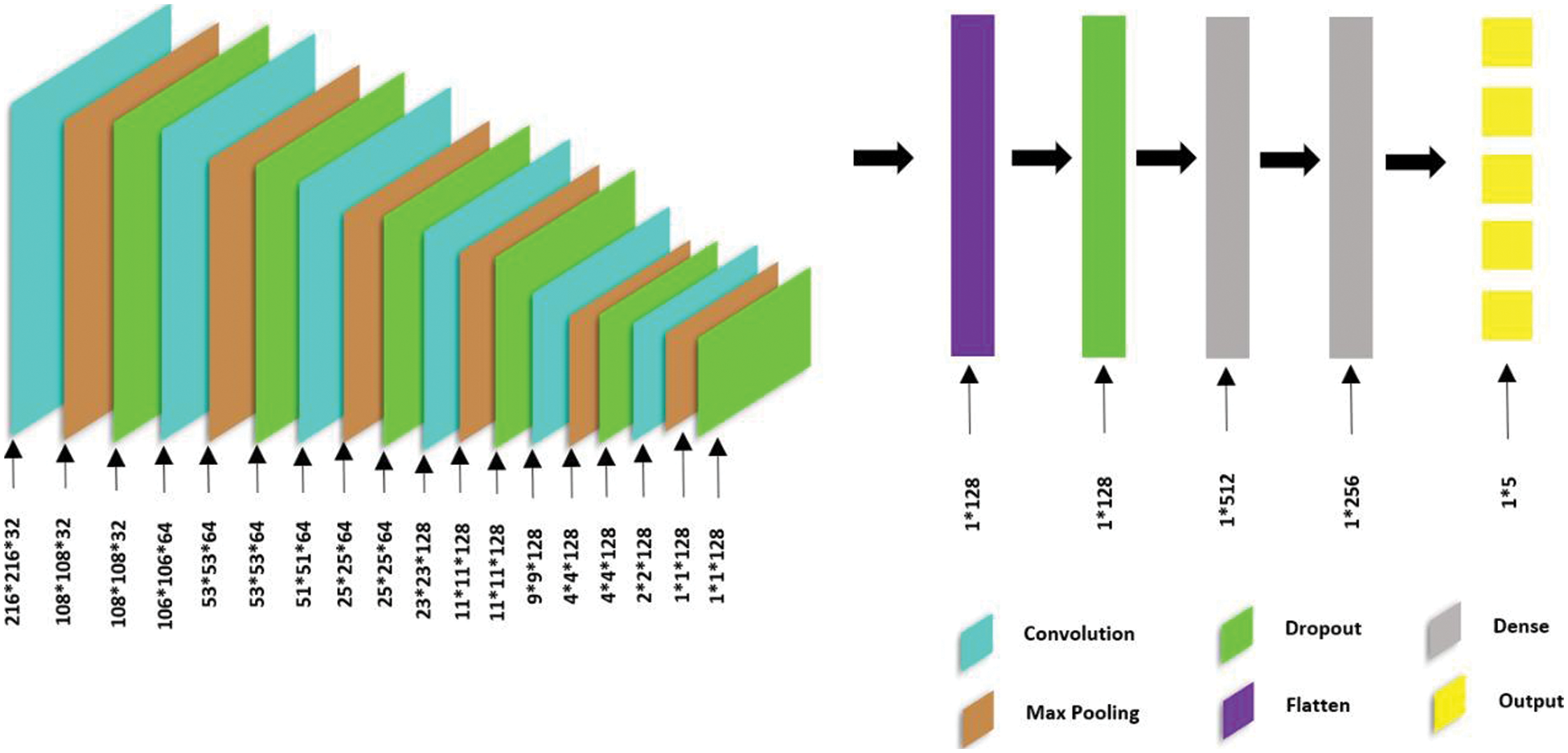
Figure 7: CNN architecture with 6 convolutional layers

3.3.2 CNN-LSTM

LSTM networks are a form of RNN capable of learning long-term dependencies. An LSTM network can be used to train a deep neural network to classify sequence data. Typically, this network allows to feed sequence data into a network and creates predictions based on the sequence data’s discrete time steps. LSTMs cannot be used to classify images on their own. This is where CNN enters the picture. In image classification, the hybrid architecture of CNN and LSTM can be used: LSTM is used as a classifier, and CNN is used to extract complex properties from images.

Five layers of Time-Distributed Convolutional (TDC) layers, along with an LSTM layer, make up the proposed CNN-LSTM architecture; refer Fig. 8. The input layer is the first TDC layer having a 32-bit block size, a 5 × 5 kernel size, and ReLu activation. This layer is followed by two TDC layers, each having a 3 × 3 kernel and a block size of 64. Finally, two more TDC layers with a block size of 128 and a kernel similar to the preceding levels are added. All the TDC layers use the ReLu activation function, and they’re followed by a 2 × 2 Max Pooling layer and a 0.1 decay Dropout layer. Following these layers, a flattening layer is used to compress the two-dimensional features into a single dimension. The LSTM layer that follows uses a dropout rate of 0.4. The model’s final components are ANN layers with 256 and 5 neurons, respectively, with the former implementing ReLU activation and the latter using the sigmoid activation function. The Adam optimizer is used to compile the model, and the loss is set to Categorical Cross Entropy.

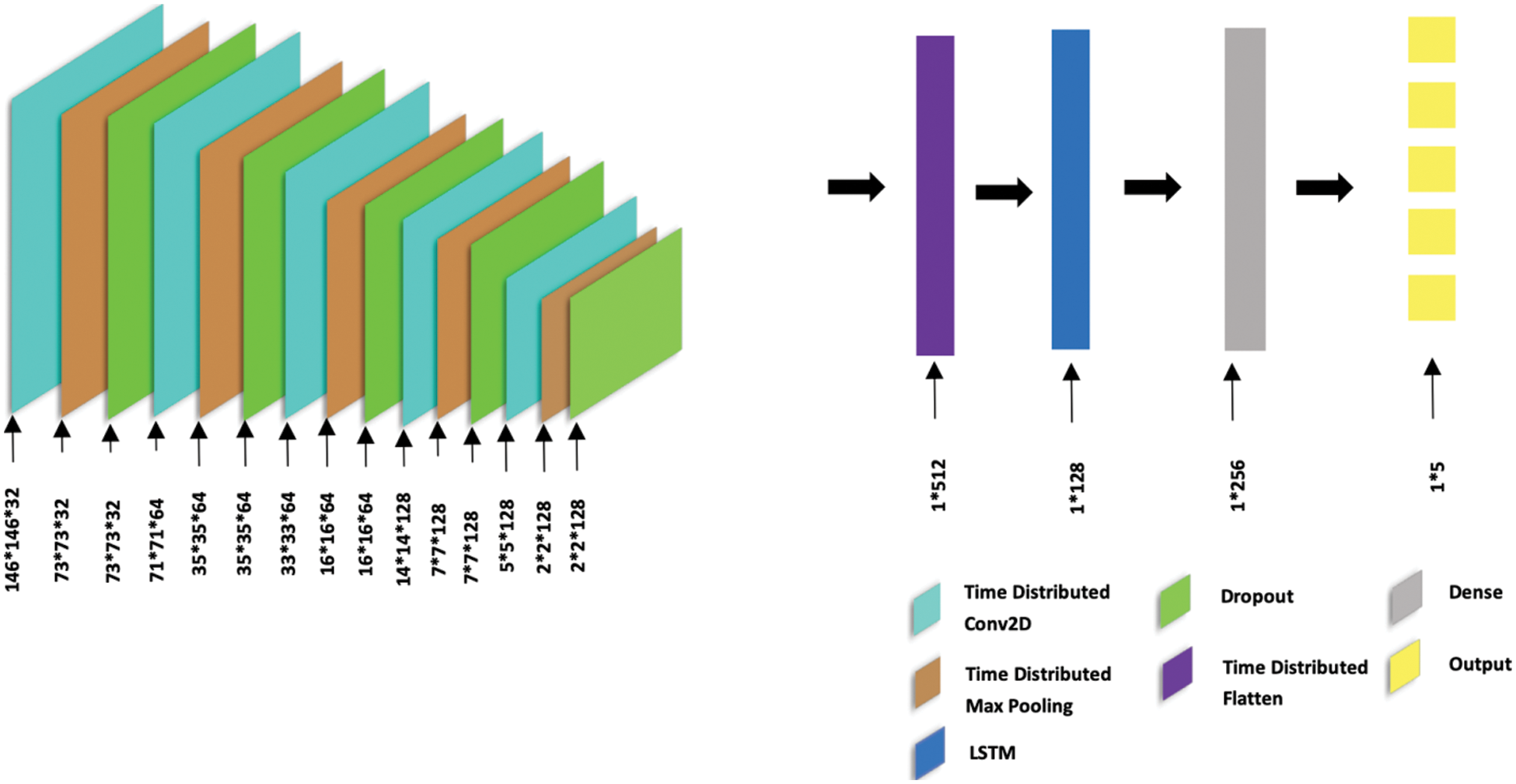
Figure 8: CNN-LSTM architecture with 5 TDC (Time-Distributed Convolutional) layers

3.4 Transfer Learning Models

All the comparison models are CNN-based models that have been pre-trained on the ImageNet dataset, which is said to contain over a million images. All of the transfer-learning models follow the same structure, are free to use, and can be downloaded. To use any of the pre-trained models, the input data shape must be fed to the model.

3.4.1 MobileNetv2

MobileNetV2 is a CNN model with 53 layers. This trained model was created with the goal of performing well on mobile devices. The MobileNetV2 model with average pooling and ImageNet weights is imported using Tensorflow. The model structure is as defined: all of the top layers are fixed, a dropout layer is added to control noise, and a five-output layer with a SoftMax activation function is implemented. Stochastic Gradient Descent (SGD) is used to optimize the model, and categorical cross-entropy is used as the loss function. The model is trained over 150 epochs with a 0.2 validation split.

3.4.2 VGG16

VGG16 is a CNN model composed of 16 layers. The VGG16 model requires an input image that is 224 × 224 pixels in size, with colored images requiring three channels. Even though the input images are binary, they are converted into an RGB model in order to train using transfer learning models. There are 13 convolutional layers, pooling layers, and three fully connected layers in the model. The VGG16 model with ImageNet weights is imported using Tensorflow. The model is summarized as follows: all top layers are fixed; a flattening layer to flatten the output image; a fully connected dense layer to assign weights with the ReLu activation function; a dropout layer to suppress noise; and an output layer with five outputs with a SoftMax activation function. The network is designed utilizing Adam as the optimizer and categorical cross-entropy as the loss function. With a 0.2 validation split, the network is trained across 250 epochs.

3.4.3 VGG19

VGG19 is another variation of the VGG architecture. The model is made up of 19 layers, as the name indicates. There are 16 convolutional layers, 5 maximum pooling layers, and 3 fully connected layers used in this model. The VGG16 model requires an input image that is 224 × 224 pixels in size, with colored images requiring three channels. Even though the input images are binary, they are converted into an RGB model in order to train in transfer learning models. The VGG19 model with ImageNet weights is imported using Keras. The model is similar to VGG16-all the top layers are fixed; a flattening layer to flatten the output image; three fully linked dense layers to assign weights with the activation function ReLU; and an output layer with five outputs with the activation function SoftMax. Adamax is used to optimize the network, and binary cross-entropy is used as the loss function. After that, the network is trained with a 0.2 validation split over seven epochs.

3.4.4 InceptionV3

InceptionV3 is yet another CNN-based image recognition model that is pre-trained on the ImageNet dataset. It consists of 48 layers, and the model with ImageNet weights is imported using Tensorflow. All the top layers of the model are fixed, followed by a flattening layer to flatten the output image; a fully connected dense layer to assign weights with the ReLu activation function; a dropout layer to suppress noise; and an output layer with ten outputs with the Sigmoid activation function. The network is designed utilizing Root Mean Squared Propagation (RMSprop) as the optimizer and binary cross-entropy as the loss function. With a 0.2 validation split, the network is trained across 75 epochs.

3.4.5 ResNet50

ResNet denotes a Residual Network. ResNet50 is a ResNet model variation with 48 convolution layers, one MaxPool layer, and one Average Pool layer. The ResNet 50 design is much more precise than the 34-layer ResNet model. Tensorflow is used to import the ResNet50 model with ImageNet weights. The model is made up of fixed-top layers, a flattening layer to flatten the output image, a fully connected dense layer to assign weights with the ReLu activation function, a dropout layer to suppress noise, and an output layer with five outputs and the SoftMax activation function. The network is built with Adam as the optimizer and sparse categorical cross-entropy as the loss function. With a 0.25 validation split, the network is trained across 250 epochs.

3.4.6 ResNet9

Another variation of the Residual Network is the ResNet9. As the name suggests, it has 9 layers in total: 4 convolutional layers, 2 residual layers (each consisting of two convolutional layers), and 1 linear layer. A batch normalization layer is added after each convolutional layer to normalize the output from the preceding layer. This model with ImageNet weights, unlike the ResNet50, is imported using Pytorch. However, ResNet9 has a similar architecture to ResNet50, with fixed-top layers, a flattening layer to flatten the resulting image, a fully connected dense layer to attribute weights with the ReLu activation function, a dropout layer to bring down the noise, and a five-output output layer with the SoftMax activation function. Adam is used as the optimizer, while sparse categorical cross-entropy is used as the loss function. With a 0.25 validation split, the network is trained across 250 epochs.

4  Results and Discussions

4.1 Effect of Epochs

All models are trained across 250 epochs. The results of the training process are visualized in Fig. 9. The transfer learning model ResNet9 performs best followed by the proposed CNN-LSTM model. The proposed CNN model performs closely better following the CNN-LSTM model. The ResNet50 and MobileNetV2 models lag behind the bunch which can be attributed to their dated architecture. This model has been surpassed by newer and more complex models. All models generally peak around 100 to 150 epochs and further training causes overfitting, which explains the dip in accuracy after a certain number of epochs.

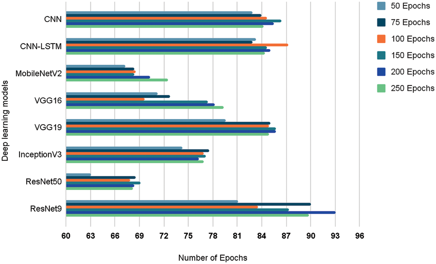
Figure 9: Validation accuracy of each model across 250 epochs (%)

The only exceptions to these trends are the MobileNetV2, VGG16 and ResNet9 models. These models learn at a slower rate and take a longer time to reach convergence. The transfer learning models overfit to a lesser extent than the proposed networks. This characteristic can be explained by the fact that the transfer learning models have been trained on a large standard and therefore are able to generalize better. However, this is also what holds the models back from performing as well as the proposed models on the given data.

Table 1 given above gives more insight into the exact accuracy of each model at the given epoch checkpoints of 50, 75, 100, 150, 200 and 250. ResNet9 gives the best accuracy of 93.06% with 200 epochs. However, there is a slight drop in accuracy during its 250th epoch. The proposed CNN-LSTM model achieves its maximum performance of 87.25% accuracy at the 100th epoch before dropping off. The proposed CNN model achieves a performance of 86.37% at the 150th epoch.

The ResNet50 model learns at a slower rate and reaches its maximum accuracy of 69.16% after the completion of 150 epochs. Similarly, even the MobileNetV2 transfer learning model achieves its maximum performance of 72.53% accuracy after completing the entire 250 epochs. Following this, VGG16 model shows the best accuracy of 79.34% with 250 epochs. The improved VGG19 model however reached peak performance at 150 epochs with an accuracy of 85.71%.

Interestingly the model achieves the exact same accuracy after the completion of 200 epochs. The final transfer learning model InceptionV3 reaches its highest performance of 77.58% relatively soon after the completion of 75 epochs. The performance of the model largely remains the same after 75 epochs due to the reasons mentioned previously. Overall, the model with the maximum performance seems to be the proposed ResNet9 model with an accuracy of 93.06%. It is to be noted that further experimentation is done by training each of the models up to the respective epoch in which the particular model achieves maximum performance.

4.2 With and Without Data Augmentation

Table 2 provides the accuracy of each model after augmenting the dataset that they are trained on. Fig. 10 shows the effect of data augmentation on each model. The outcomes are polarized. On one hand, the performance of models like the proposed CNN model has surged, while models like CNN-LSTM have had abysmally low performance. Transfer learning models like the VGG16, ResNet50, and ResNet9, show better performance after augmentation, while MobileNetv2, VGG19, and InceptionV3 models work better before augmentation.

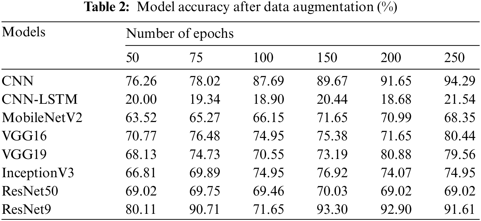
Figure 10: Best accuracy of each model before and after augmentation (%)

This discrepancy can be explained by the fact that data augmentation sometimes causes the models to overfit. This is especially true in the case of the proposed CNN-LSTM model, which exhibits an exceptional training accuracy of 96.26%. However, this is yet another case of the model overfitting the training data, as can be seen from the low accuracy of 21.54% on the testing data. The transfer learning models, due to their ability to generalize, largely avoid the overfitting seen in the proposed CNN-LSTM model. However, this also translates to slightly poorer performance.

There are four models that benefit from the data augmentation process. These models are robust, do not overfit, and exhibit the highest accuracy after augmentation. It is to be noted that further experimentation is done by training the models to the maximum accuracy achieved till now for each, respectively. For example, further experimentation with the proposed CNN model is by first training it to 250 epochs with augmented data, but the proposed CNN-LSTM model is trained to 100 epochs on un-augmented data.

4.3 Effects of Number of Convolutional Layers

The first layer of a convolutional network is the convolutional layer. After the convolutional layer, there can be either pooling or convolutional layers, but the final layer is always the dense layer. In this comparison study, the convolution layer and max-pooling layers are changed in order to observe the change in accuracy the model produces. The proposed models, CNN and CNN-LSTM, feature convolutional and max-pooling layers. It was previously observed that CNN gave better results after data augmentation with 250 epochs, and CNN-LSTM was efficient before augmentation at around 100 epochs.

Hence, by setting the best values for each model, the convolution and max-pooling layers are altered to obtain better accuracy. In the CNN model, it gives an accuracy of 86.81%, 91.65%, and 94.29% using 4, 5, and 6 layers for convolution layers, respectively. Similarly, for the CNN-LSTM model, the accuracy using 4, 5, and 6 convolution layers is 82.20%, 86.59%, and 87.25%, respectively. Table 3 shows the accuracies for each number of convolution layers for CNN and CNN-LSTM models. For better visualization, the same is represented as a graph in Fig. 11.

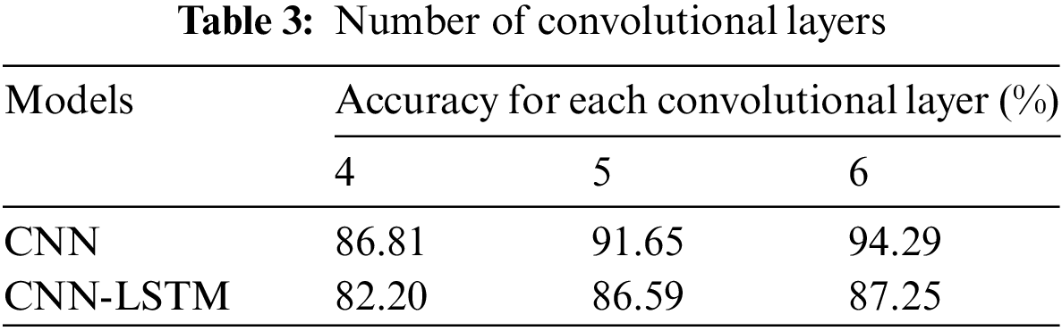
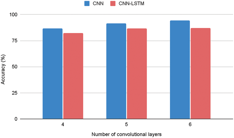
Figure 11: Accuracy of CNN and CNN-LSTM with change in number of convolutional layers

It’s important to note that the accuracy of the models improves as the number of convolutional layers increases. Both CNN and CNN-LSTM models exhibit this pattern. As the number of convolutional layers increases, the model’s complexity also increases since the number of parameters in the layers increase. Adding more layers also aids in the extraction of more features. This does not always imply that increasing the number of convolutional layers will improve accuracy. It is determined by the size of the dataset. If the dataset is too little, the model will overfit by adding additional layers.

Since the dataset used is big enough, by adding more layers, the model doesn’t overfit. The results of a comparison analysis based on the number of convolutional layers show that as the number of convolutional layers increases, the model’s accuracy improves. It can be concluded that both CNN and CNN-LSTM models give their best performance with 6 convolutional layers.

4.4 Effects of Number of Dropout Layers

At each step during the training period, the dropout randomly deems some number of layer outputs out of the network, preventing overfitting. It is a popular regularization method to improve the generalization of the model. By using dropout layers, the nodes within a layer are compelled to assume responsibility for the input layers on the basis of probability.

Dropouts may be used to generalize most sorts of layers, including fully connected layers, convolutional layers, and recurrent layers like the LSTM layer. However, it cannot be used on the output layer of any model since it refers to the plausibility of the outputs from a layer being kept. The value of the rate ranges from 0 to 1, with 1.0 meaning no outputs are dropped, and 0.0 implying the layer’s outputs are not considered.

Table 4 shows the number of dropout layers and the corresponding accuracy. Fig. 8 shows the trend in the accuracy when dropout layers are increased. This trend is observed with the help of increasing the number of dropout layers in the CNN and CNN-LSTM models. From Table 4 and the graph in Fig. 12, it is evident that the accuracy seems to be increasing at a slow rate. The dropout rate used is 0.1, throughout all layers, and the dropout passed as a parameter to the LSTM layer has a rate of 0.4. Increasing the dropout rates increases the complexity of the model.

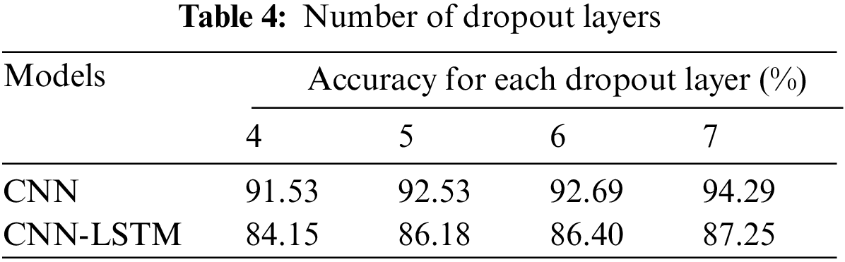
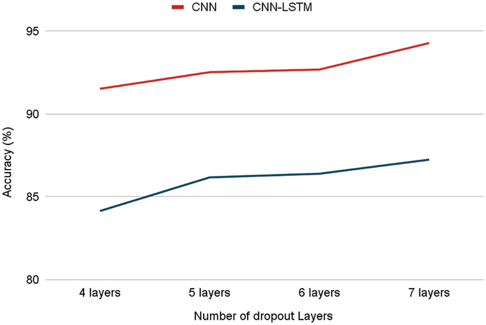
Figure 12: Accuracy of models after changing the number of dropout layers

But, due to the well-known problem of overfitting, increased complexity does not always imply higher pricing accuracy. The accuracy almost maintains a straight line with the maximum value being 94.29% for CNN and 87.25% for CNN-LSTM. If the complexity is further increased, performance on training improves but it may lead to overfitting.

4.5 Effects of Regularization

Regularization is a technique for calibrating machine learning models to ensure low error rates and lessen the danger of overfitting or underfitting. Different regularization techniques are available for training and testing deep learning models. The proposed methodology used the three regularization techniques that are Ridge Regression (L2), Data augmentation, and Dropout. Dropout is perhaps the most fascinating sort of regularization procedure. Table 5 shows the model accuracy with or without L2. This regularization delivers excellent outcomes and is therefore the most often involved procedure in deep learning. Every iteration has an alternate arrangement of nodes which allows for an alternate arrangement of results.

By setting the number of dropout layers to 7, the CNN model achieved an overall accuracy of 94.29%, whereas the CNN-LSTM model achieved an accuracy of 87.25%. Another regularization approach is data augmentation, which is the most basic way to prevent overfitting. Data augmentation significantly boosted the performance of the CNN model from 84.18% to 94.29%.

Fig. 13 demonstrates the suggested model’s accuracy before and after L2 regularization. The introduction of L2 regularization diminishes the efficacy of both recommended models for the CASIA dataset, demonstrating that L2 regularization is not necessary for CNN and CNN-LSTM. CNN’s greatest accuracy was 94.29% without L2, after data augmentation at seven dropout layers, compared to CNN-LSTM’s accuracy of 87.25% without L2, without augmentation, and at seven dropouts.

Figure 13: Accuracy of the model before and after L2 regularization

4.6 Effects of Optimizers

The CNN model performs exemplarily when Adam is used as the optimizer. Since adaptive moment estimation is more efficient when it comes to working with problems involving large amounts of data and parameters, it results in better accuracy. The images here are converted into RGB values which results in a matrix of order 220 × 220 each where each element is a list of length 3. It also requires less memory, and it is efficient.

However, the model gives a very low accuracy when compiled with SGD as the optimizer. This may be due to the frequent updates which cause the steps that were taken towards the minima to be very noisy. Due to this, the gradient descent leans in other directions. Here the images are converted to vectors. SGD loses the upper hand in vectorized operations because it can only operate with a single example at a time.

The other optimizers, namely Adamax, RMSprop and Nadam give a similar accuracy in the range of 80% to 90% approximately. Table 6 shows the accuracy of different models upon using multiple optimizers. The same is expressed as a graph in Fig. 14.

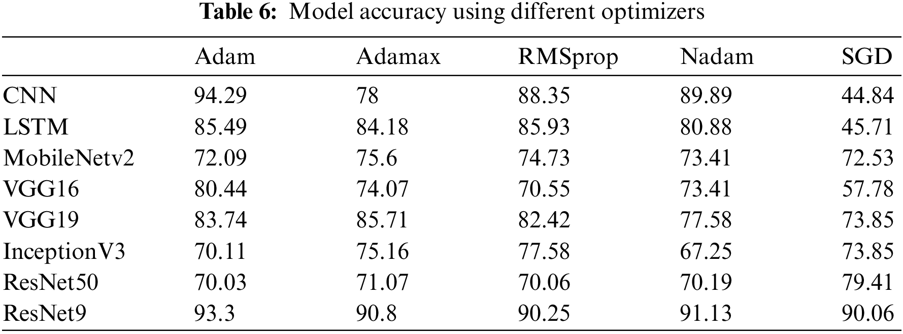
Figure 14: Accuracy of each model using different optimizers

The use of Adam Optimizer for VGG16 and ResNet9 also expressed the maximum accuracy out of all other optimizers. Similarly, SGD performs the least out of all other optimizers due to the fact that Adam performs innate coordinate-wise gradient trimming and can thus handle heavy-tail noise, unlike SGD.

When RMSprop is used as the optimizer for the CNN-LSTM model, the accuracy observed is the highest when compared with other optimizers. This is the case because RMSprop is an adaptive learning optimization algorithm that is used for RNNs, which are sequential models. It overcomes the vanishing or exploding problem of gradients by using a moving average of squared gradients to normalize the gradient itself.

Due to the shortcoming discussed earlier, SGD also gives the lowest accuracy for this model. The Adam optimizer’s accuracy is very close to the highest value since it also solves the vanishing gradient problem, similar to RMSprop. The other optimizers yield respectable accuracy, with 80.88 and 84.18 by Nadam and Adamax, respectively.

The same reasoning can be applied to the InceptionV3 transfer learning model, as RMSprop performs the best out of the other optimizers for this model. It is observed that for ResNet50, ResNet9, and MobileNetV2, all the optimizers show similar performances. The Adam optimizer performs the best for ResNet9, Adamax expresses the best in MobileNetV2 and VGG19, and SGD brings out the best in ResNet50.

Since Adamax accelerates the optimization process, it outperforms the Adam optimizer in the case of VGG19 and MobileNetV2. SGD works better in cases of generalization as opposed to Adam. Thus, it can be concluded that ResNet9 provides a model accuracy that is comparable to that of the proposed CNN model.

5  Conclusion

Analyzing human gait is an important research topic with a lot of potential for applications in medicine, biometrics, sports, and other areas. The CASIA B and CASIA C datasets were used to perform gait classification in this research. There were two models proposed: CNN and CNN-LSTM. Six transfer learning models were used to evaluate the proposed models’ performance. They are MobileNetV2, InceptionV3, VGG16, VGG19, ResNet9, and ResNet50.

Multiple comparisons were carried out step by step using various measures such as the number of epochs, before and after data augmentation, number of convolutional layers, number of dropout layers, regularization, and different optimizers.

From all the experiments conducted, it is evident that the CNN model outperforms all other models with an accuracy of 94.29%. It achieved the best accuracy at its 250th epoch after data augmentation using 6 convolutional and 7 dropout layers. Moreover, it showed a notable performance without regularization and using Adam as its optimizer.

Following the CNN model, the ResNet9 model gave a significant performance with an accuracy of 93.3%. Following this, the proposed CNN-LSTM achieved an accuracy of 87.25% without augmentation, and without L2 regularization using 7 dropout layers and 6 convolutional layers at the 100th epoch. ResNet50 had the lowest accuracy (70.03%), indicating that it is not the best transfer learning model for this case.

This study may be explored further by focusing on gait, which depicts various angles of human walking. More data may be used to improve accuracy with the aid of better system design. Only silhouette images are employed for gait analysis in this study. To enhance categorization, an image dataset with people of varying ages, genders, heights, and weights may be used.

Acknowledgement: Deepest gratitude to the Institute of Automation, Chinese Academy of Sciences (CASIA) for providing the CASIA Gait Database that was used for gait recognition and classification in this research.

Funding Statement: The authors received no specific funding for this study.

Conflicts of Interest: The authors declare that they have no conflicts of interest to report regarding the present study.

References

1. C. L. Hugos and H. M. Cameron, “Assessment and measurement of spasticity in MS: State of the evidence,” Current Neurology and Neuroscience Reports, vol. 19, no. 10, pp. 1–7, 2019. [Google Scholar]
2. I. U. Isaias, M. Dipaola, M. Michi, A. Marzegan, J. Volkmann et al., “Gait initiation in children with rett syndrome,” PLoS One, vol. 9, no. 4, pp. e92736, 2014. [Google Scholar]
3. M. A. Khan, S. Kadry, P. Parwekar, R. Damaševičius, A. Mehmood et al., “Human gait analysis for osteoarthritis prediction: A framework of deep learning and kernel extreme learning machine,” Complex & Intelligent Systems, vol. 8, pp. 1–19, 2021. [Google Scholar]
4. J. Wu, K. Kuruvithadam, A. Schaer, R. Stoneham, G. Chatzipirpiridis et al., “An intelligent in-shoe system for gait monitoring and analysis with optimized sampling and real-time visualization capabilities,” Sensors, vol. 21, no. 8, pp. 2869, 2021. [Google Scholar]
5. M. Hnatiuc, O. Geman, A. G. Avram, D. Gupta and K. Shankar, “Human signature identification using IoT technology and gait recognition,” Electronics, vol. 10, no. 7, pp. 852, 2021. [Google Scholar]
6. J. A. P. De la Mora, “Instrumented footwear and machine learning for gait analysis and training,” Ph.D. Dissertation, Columbia University, 2021. [Google Scholar]
7. R. B. Davis III, S. Ounpuu, D. Tyburski and J. R. Gage, “A gait analysis data collection and reduction technique,” Human Movement Science, vol. 10, no. 5, pp. 575–587, 1991. [Google Scholar]
8. V. C. D. Lima, V. H. Melo and W. R. Schwartz, “Simple and efficient pose-based gait recognition method for challenging environments,” Pattern Analysis and Applications, vol. 24, no. 2, pp. 497–507, 2021. [Google Scholar]
9. A. Khan, M. Y. Javed, M. Alhaisoni, U. Tariq, S. Kadry et al., “Human gait recognition using deep learning and improved ant colony optimization,” Computers, Materials & Continua, vol. 70, pp. 2113–2130, 2022. [Google Scholar]
10. R. Aznar-Gimeno, G. Labata-Lezaun, A. Adell-Lamora, D. Abadía-Gallego, R. del-Hoyo-Alonso et al., “Deep learning for walking behaviour detection in elderly people using smart footwear,” Entropy, vol. 23, no. 6, pp. 777, 2021. [Google Scholar]
11. R. A. Espinosa, W. H. Angulo, H. D. Fuentes and A. J. Rincón, “Insole of footwear instrumented to evaluate the parameters related to gait and weight using a digital or mobile technology,” in 2021 Global Medical Engineering Physics Exchanges/Pan American Health Care Exchanges (GMEPE/PAHCE), Sevilla, Spain, pp. 1–4, 2021. [Google Scholar]
12. Q. Zou, Y. Wang, Q. Wang, Y. Zhao and Q. Li, “Deep learning-based gait recognition using smartphones in the wild,” IEEE Transactions on Information Forensics and Security, vol. 15, pp. 3197–3212, 2020. [Google Scholar]
13. A. S. Alharthi, S. U. Yunas and K. B. Ozanyan, “Deep learning for monitoring of human gait: A review,” IEEE Sensors Journal, vol. 19, no. 21, pp. 9575–9591, 2019. [Google Scholar]
14. A. Kececi, A. Yildirak, K. Ozyazici, G. Ayluctarhan, O. Agbulut et al., “Implementation of machine learning algorithms for gait recognition,” Engineering Science and Technology, an International Journal, vol. 23, no. 4, pp. 931–937, 2020. [Google Scholar]
15. H. Zhang, Y. Guo and D. Zanotto, “Accurate ambulatory gait analysis in walking and running using machine learning models,” IEEE Transactions on Neural Systems and Rehabilitation Engineering, vol. 28, no. 1, pp. 191–202, 2019. [Google Scholar]
16. A. Peinado-Contreras and M. Munoz-Organero, “Gait-based identification using deep recurrent neural networks and acceleration patterns,” Sensors, vol. 20, no. 23, pp. 6900, 2020. [Google Scholar]
17. A. M. Saleh and T. Hamoud, “Analysis and best parameters selection for person recognition based on gait model using CNN algorithm and image augmentation,” Journal of Big Data, vol. 8, no. 1, pp. 1–20, 2021. [Google Scholar]
18. A. Turner and S. Hayes, “The classification of minor gait alterations using wearable sensors and deep learning,” IEEE Transactions on Biomedical Engineering, vol. 66, no. 11, pp. 3136–3145, 2019. [Google Scholar]
19. S. S. Lee, S. T. Choi and S. I. Choi, “Classification of gait type based on deep learning using various sensors with smart insole,” Sensors, vol. 19, no. 8, pp. 1757, 2019. [Google Scholar]
20. A. Saboor, T. Kask, A. Kuusik, M. M. Alam, Y. Le Moullec et al., “Latest research trends in gait analysis using wearable sensors and machine learning: A systematic review,” IEEE Access, vol. 8, pp. 167830–167864, 2021. [Google Scholar]
21. I. Orović, S. Stanković and M. Amin, “A new approach for classification of human gait based on time-frequency feature representations,” Signal Processing, vol. 91, no. 6, pp. 1448–1456, 2011. [Google Scholar]
22. N. M. Tahir and H. H. Manap, “Parkinson disease gait classification based on machine learning approach,” Journal of Applied Sciences, vol. 12, no. 2, pp. 180–185, 2012. [Google Scholar]
23. L. Wang, R. Han, J. Chen and W. Feng, “Combining the silhouette and skeleton data for gait recognition,” Computer Vision and Image Understanding, vol. 2, pp. 1–10, 2022. [Google Scholar]
24. J. Amin, M. A. Anjum, M. Sharif, S. Kadry, Y. Nam et al., “Convolutional Bi-LSTM based human gait recognition using video sequences,” Computers, Materials & Continua, vol. 68, no. 2, pp. 2693–2709, 2021. [Google Scholar]
25. S. Zheng, J. Zhang, K. Huang, R. He and T. Tan, “Robust view transformation model for gait recognition,” in Int. Conf. on Image Processing(ICIP), Brussels, Belgium, 2011. [Google Scholar]
26. S. Yu, D. Tan and T. Tan, “A framework for evaluating the effect of view angle, clothing and carrying condition on gait recognition,” in Proc. of the 18th Int. Conf. on Pattern Recognition (ICPR), Hong Kong, China, 2006. [Google Scholar]
27. D. Tan, K. Huang, S. Yu and T. Tan, “Efficient night gait recognition based on template matching,” in Proc. of the 18th Int. Conf. on Pattern Recognition (ICPR06), Hong Kong, China, 2006. [Google Scholar]
28. G. Bradski, “The openCV library,” Dr. Dobb’s Journal: Software Tools for the Professional Programmer, vol. 25, no. 11, pp. 120–123, 2000. [Google Scholar]
29. M. Sandler, A. Howard, M. Zhu, A. Zhmoginov and L. C. Chen, “Mobilenetv2: Inverted residuals and linear bottlenecks,” in Proc. of the IEEE Conf. on Computer Vision and Pattern Recognition, Salt Lake City, UT, USA, pp. 4510–4520, 2018. [Google Scholar]
30. K. Simonyan and A. Zisserman, “Very deep convolutional networks for large-scale image recognition,” Computer Vision and Pattern Recognition, vol. 1409, no. 1556, pp. 1–14, 2014. [Google Scholar]
31. C. Szegedy, V. Vanhoucke, S. Ioffe, J. Shlens and Z. Wojna, “Rethinking the inception architecture for computer vision,” in Proc. of the IEEE Conf. on Computer Vision and Pattern Recognition, Las Vegas, NV, USA, pp. 2818–2826, 2016. [Google Scholar]
32. K. He, X. Zhang, S. Ren and J. Sun, “Deep residual learning for image recognition,” in Proc. of the IEEE Conf. on Computer Vision and Pattern Recognition, Las Vegas, NV, USA, pp. 770–778, 2016. [Google Scholar]
Cite This Article
Copyright © 2023 The Author(s). Published by Tech Science Press.
This work is licensed under a Creative Commons Attribution 4.0 International License , which permits unrestricted use, distribution, and reproduction in any medium, provided the original work is properly cited.
Downloads
Citation Tools