Feature-Limited Prediction on the UCI Heart Disease Dataset

1  Introduction

According to the World Health Organization (WHO), cardiovascular diseases (CVDs), commonly known as heart diseases, are the leading causes of death globally. In 2016, the total death count reached about 58 million people, 31% of whom died due to CVDs. Most of these deaths, around 85%, were from heart attacks and strokes [1]. WHO has put a worldwide action plan spanning 2013 to 2020 in response to CVDs and cancer, diabetes, and chronic respiratory diseases, collectively known as Noncommunicable diseases (NCDs). The goal is to attain a 25% relative reduction in premature death from NCDs by 2025. These efforts are necessary steps toward fighting this on a global scale. However, humanity needs awareness on a more individual level. For example, the American Health Association has reported several behavioral risk factors that can be regulated to prevent CVDs, such as smoking cigarettes, eating unhealthy food, and not exercising regularly. High cardiovascular risk patients suffering from hypertension, diabetes, and/or hyperlipidemia should be closely monitored as early detection of CVDs can prevent premature deaths [2]. Many of these risk factors can be easily measured using accessible tools that might be part of any modern household. Moreover, with the advancement of technology, there are even now smartwatches and wearables equipped with health-tracking sensors. Every factor alone might not be a good indicator of heart disease, but their interaction can provide a clearer signal to the health counselor or the doctor [3]. Developing systems that can assist human professionals in monitoring high-risk patients is a good strategy for performing widespread testing for CVDs and devising proactive measures [4]. To enable such application without losing utility, it is imperative to use as less information about the patient as possible.

With the rise of the Artificial Intelligence (AI) era, many data-driven problems have become possible to solve with expert accuracy. Most of the recent success can be attributed to the advances in Machine Learning (ML), a subfield of AI that relies heavily on abundant data. To that end, using datasets that contain patients’ information with and without CVDs, such as the UCI Heart Disease Dataset [5], is essential to applying ML algorithms. However, analyzing these datasets requires cleaning and preprocessing. This work proposes different approaches to classify early whether a patient has heart disease using classical and modern ML methods with the help of some Data Mining (DM) techniques. Finally, it will perform ablation studies to determine the most distinctive features of CVDs.

2  Related Work

To reliably diagnose heart diseases in a patient, a doctor needs to ask some questions and run a few tests. The goal is to identify important attributes as the basis for the final diagnosis. Examples include the patient’s age, sex, type of chest pain, and resting blood pressure. In the ML community, these attributes are referred to as features. One can formulate the problem as an ML problem (precisely, a classification problem); given the input features (i.e., patient information), the goal is to predict whether the patient has cardiovascular disease (CVD) or not. The proposed system attempts to solve this problem to prevent further complications that might lead to heart failures like heart attacks and strokes [4].

2.1 Algorithms

From the DM field [6], it is known that some features are more important than others for classification. However, sometimes the combination of two weak features can be more critical than a stronger feature. All of this led to the study of feature selection methods [7]. Examples of such methods include the Relief method, Minimal-Redundancy Maximal-Relevance Algorithm, Least Absolute Shrinkage, and the Selection Operator, all of which were studied for CVDs in [8]. This research will leverage feature selection to its advantage for two main reasons. The first reason is to improve the predictive power of the proposed classifier. The second reason is to train multiple models that rely on less information which helps when specific values are hard to attain (e.g., blood pressure is unknown).

ML classifiers can be divided into classical and modern [9]. Heart disease prediction systems were developed using both methods. Examples of classical methods include K-Nearest Neighbor (KNN), Support Vector Machine (SVM) [10], and Naive Bayes (NB) [11], all of which were studied in [12]. Other classical approaches include Logistic Regression (LR) [13], Ridge Classifier (RC) [14], Linear Discriminant Analysis (LDA) [15], Gaussian Process (GP) [16], Decision Tree (DT) [17], and Random Forest (RF) [18]. Modern ML methods focus on Deep Learning (DL), the study of deep Artificial Neural Networks (ANN). Examples of ANNs include Multi-Layer Perceptron (MLP) [19] and Recurrent Neural Network (RNN) [20]. This paper will compare a few classical and modern ML methods and build a hybrid model combining multiple models, also known as the ensemble model, as in [21]. Ensembles are better since two minds are always better than one (e.g., the wisdom of the crowd). The biggest hurdle to this work is the availability of data. Since health records are considered private information, coming across useful data for research is not as easy as in other fields. Up to our knowledge, the only publicly available dataset for CVD was collected three decades ago [5]. Other datasets exist, but they require signing NDAs because of their sensitive nature. Hence, most cited work use only this dataset [22].

2.2 Contributions

The main contributions can be summarized as follows: (1) Providing exploratory data analysis on the UCI Heart Disease Dataset to study its features. (2) Following proper ML workflow to train on the entire dataset without removing patients with missing values. (3) Determining the most discriminative features of CVDs using feature selection on an ensemble model. (4) Performing a comparative study of multiple ML models and releasing a competitive model using only a few selected features. (5) Open-sourcing reproducible code for all the experiments in the supplementary material. Contemporary arts exist, such as [19] and [23]. Nevertheless, they do not train on the entire dataset and do not perform feature selection.

3  UCI Heart Disease Dataset

This dataset was collected in 1988 from four cities: Cleveland, Hungary, Switzerland, and Long Beach. It has 920 cases of people with and without CVDs with 76 attributes each. However, only 13 are used in practice, as seen in Fig. 1. The top five plots illustrate the histograms for the numerical features in the dataset. The count of patients missing the value for a particular feature is presented in the legend. The bottom plots show the categorical features in pie charts (missing values are labeled as “Unknown”).

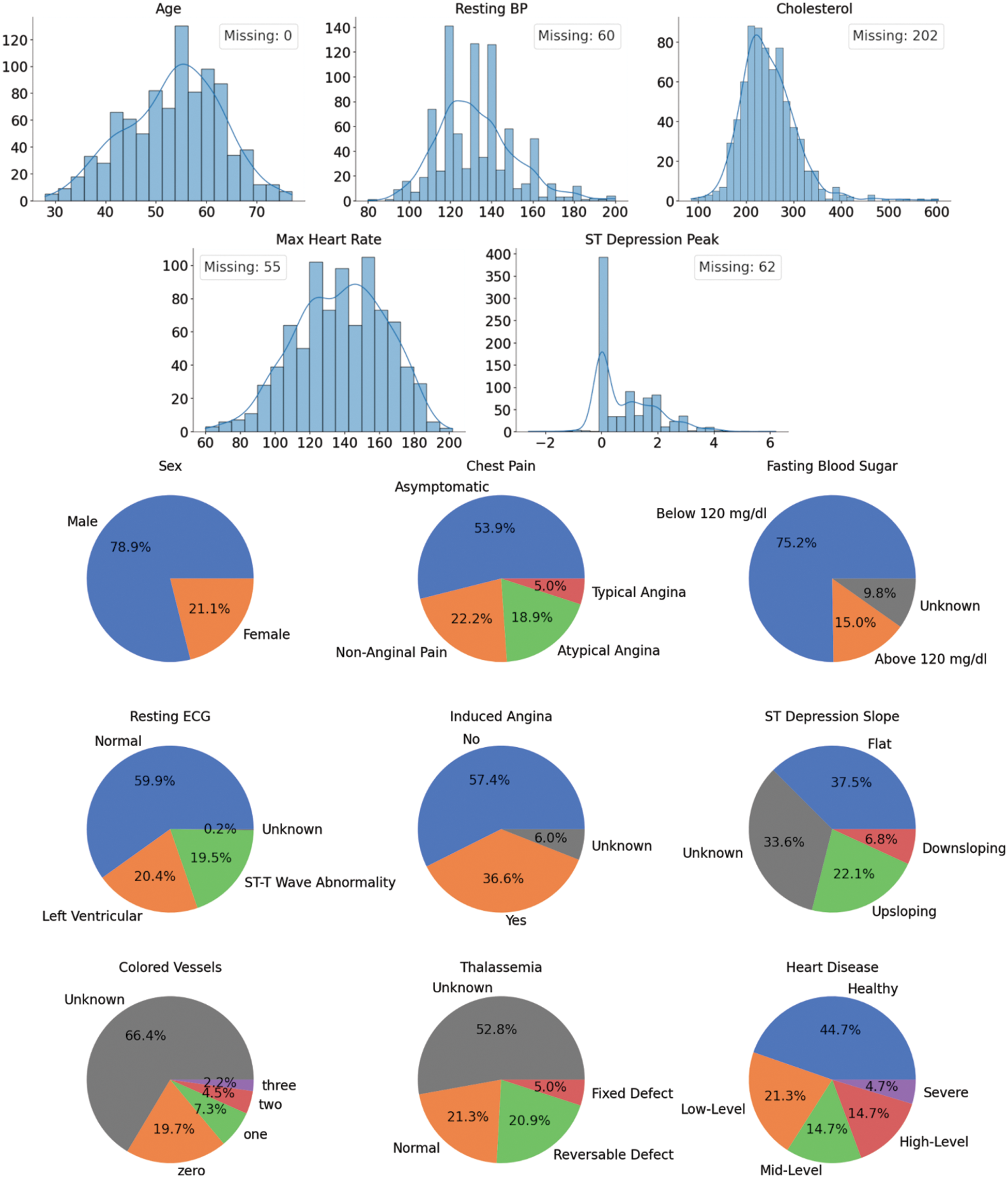
Figure 1: UCI heart disease dataset features’ distributions

After the Extract-Transform-Load (ETL) step comes performing Exploratory Data Analysis (EDA). The first thing to note here is that two-thirds of the cases have missing values. Removing them as commonly practiced is unadvisable since the dataset is already too small. In addition, the data shows five different CVDs severity levels ranging from healthy to Severe. These class labels are imbalanced, but it is possible to balance them out by changing the problem into binary classifications (two class labels: healthy and unhealthy). From this point onward, this assumption will be held to simplify the analysis. Lastly, it is essential to mention that about 80% of the patients are males. This is unlikely a truly representative sample of the real world, which might indicate a bias in the dataset. It is paramount to keep this in mind as it might have a detrimental effect on the predictive power and reliability of the trained models.

Nevertheless, one needs to see how the data is distributed given the class label to get a deeper insight into interpreting these features. Fig. 2 plots the numerical features against each other in pairs while color coding the points by whether the patients suffer from CVDs or not (missing values are ignored). The plots on the diagonal are simply the histograms of the features since the scatter plot of any feature will result in a degenerate line. It can be observed that the most discriminative features are “Max Heart Rate” and “ST Depression Peak”. In addition, there is no strong correlation between the features, which means that they encode different information and are not replaceable (no multicollinearity).

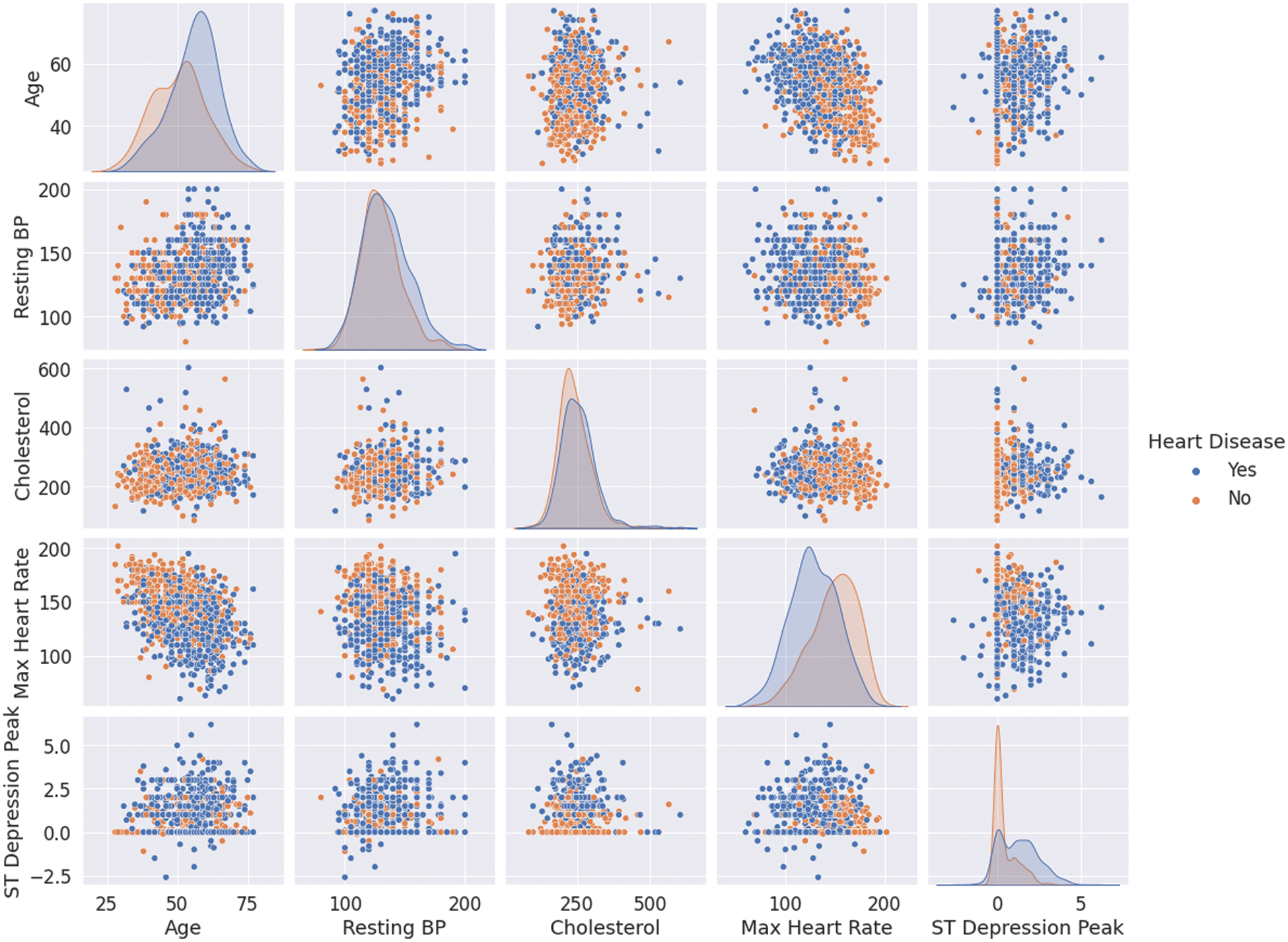
Figure 2: Numerical features’ correlations for patients with and without CVDs

The same analysis can be applied to the categorical features, as shown in Fig. 3. From these plots, it can be observed that the ratio of healthy to sick people is almost five times more in males than females. This could be true globally, but one cannot be confident of this since the data is not statistically significant. Furthermore, most patients with heart disease appear to have no chest pain, “Asymptomatic”, which shows the importance of this research. Cases like this can easily go unnoticed and undiagnosed.

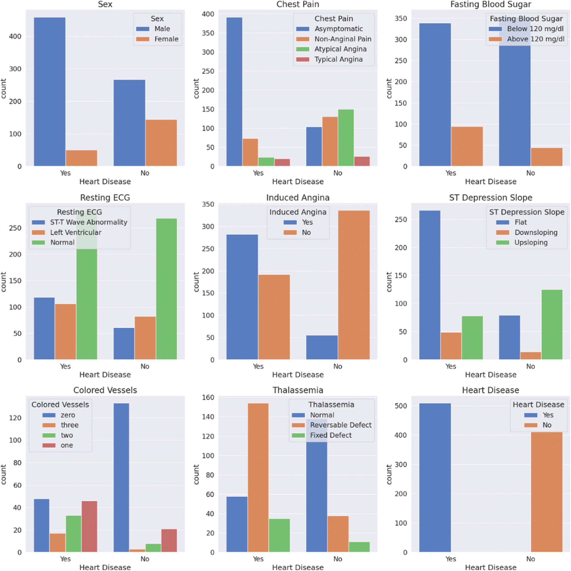
Figure 3: Categorical features’ statistics for patients with and without CVDs

4  Methodology

The proposed workflow is outlined in Fig. 4 and explained in more detail in this section.

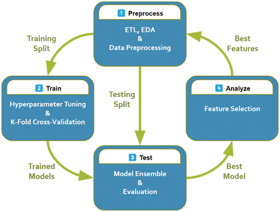
Figure 4: The proposed system pipeline

4.1 Data Preprocessing

4.1.1 Numerical Features

Since every feature has different ranges, like age and heart rate, this work will apply normalization to them. Normalization can significantly impact the trained model as it avoids preempting it to think that heart rate is more important than the person’s age. If such a relationship exists, the model should learn it on its own. To that end, the experiments will normalize the features to be zero-centered with unit variance. This is done by taking the mean μ and dividing by the standard deviation σ; x←x−μσ.

4.1.2 Categorical Features

Most ML models work strictly with numerical features. It is possible to convert categorical features into numerical features. The trick is to use one-hot encoding, an all-zeros vector with a single element being one corresponding to the index of the category.

4.1.3 Missing Values

This work replaces any missing value with the mean if it was numerical or a new class label “Unknown” if it was categorical, and the target classes are balanced by repeating randomly selected cases.

4.1.4 Data Splits

Training a complex model on simple data can result in overfitting. Informally, it is when the model can memorize the dataset entirely without learning how to classify it correctly. It is the model’s inability to detect the underlying patterns in the data. Whereas training a simple model on complex data might result in underfitting (learning trivial rules). For example, a model classifies patients based on age only (sick if old and healthy otherwise). To avoid both problematic outcomes, the data is split into two chunks. The first split will be used to train the model, and the second to test it. Both splits should be representative enough of the entire dataset (the same ratios of healthy to sick cases; stratified). A trained model is overfitting if its performance in training surpasses the testing and underfitting if it could not improve over a fixed classifier; it always predicts the same thing (healthy or sick) regardless of the input.

4.2 Training

4.2.1 Hyperparameter Tuning

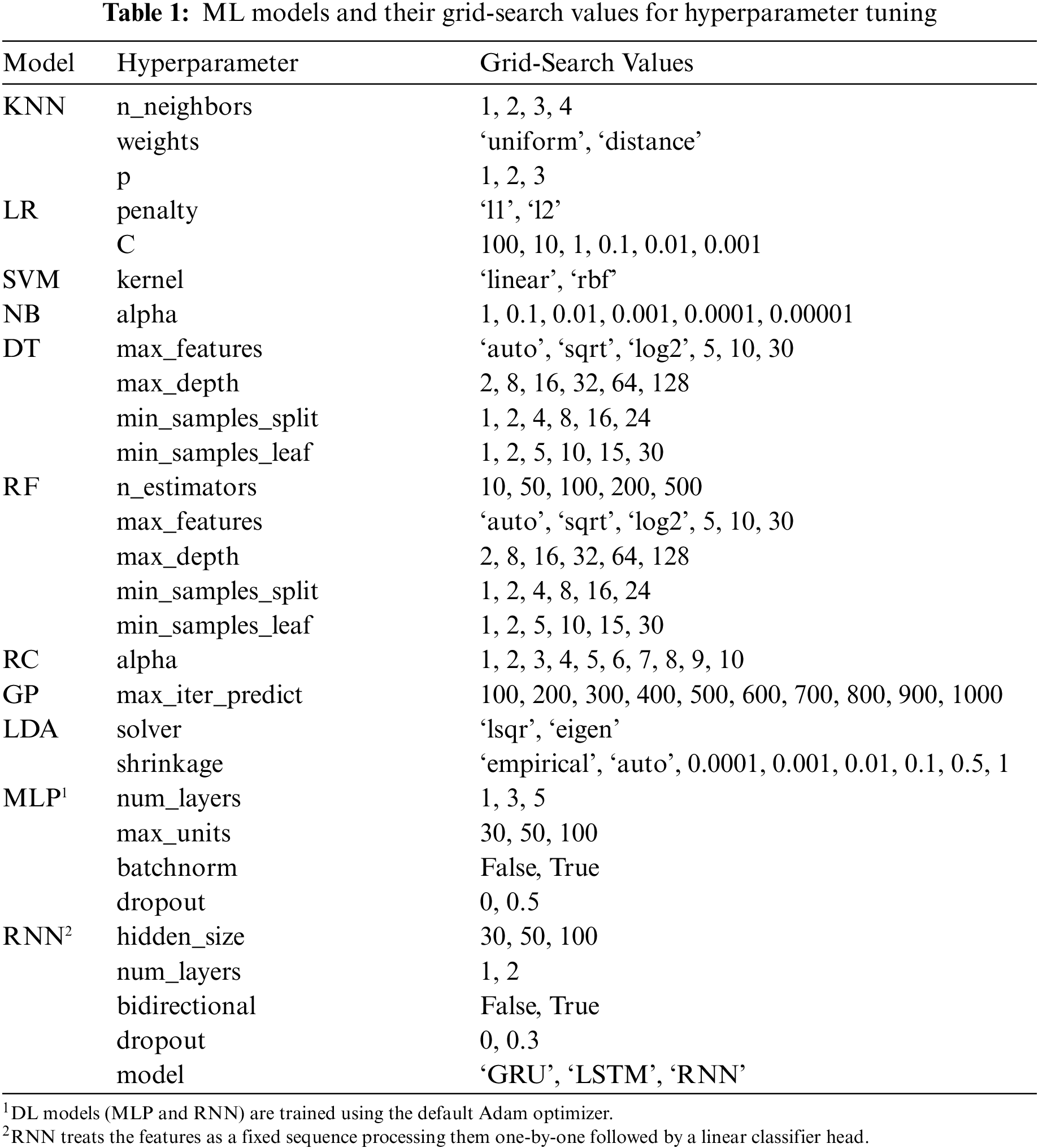
Each ML model has a few configurable hyperparameters, a set of properties that changes its training behavior and final performance. Usually, they depend on each other (e.g., a particular hyperparameter setting has a different meaning and effect if the value of another hyperparameter is changed). So, to achieve the best results for a model, it needs to be trained under all combinations of possible assigned values for its hyperparameters if feasible. This is what is known as hyperparameter tuning through grid-search. Table 1 lists the models and their grid-search values. However, it is possible to accidentally face overfitting on the test set during hyperparameter tuning (hold-out set leakage). Therefore, it is a widespread practice to tune on a small chunk of the training set, usually called the validation set.

4.2.2 K-Fold Cross-Validation

Sometimes it is not clear what constitutes a representative training-validation split. One technique is randomly splitting the training data into K chunks of equal sizes. Then, pick a single chunk for validation, and the rest K−1 chunks are combined as the training set. After that, repeat the same thing for all K chunks (every time, the validation set is a different chunk). The final score is averaged over all the K trials. This score will reflect the true strength of the model and training procedure better than an arbitrary splitting. This method is what is known as k-fold cross-validation in the ML field. It is necessary to use this score for hyperparameter tuning and only report the performance on the untouched testing set.

4.3 Model Ensemble

After building and training multiple ML models, one can compare their classifying power and see which one performs better. However, some classifiers may better classify certain types of patients than others. Therefore, choosing which classifier works best in every situation is possible. This method is an example of a model ensemble, which combines the prediction of multiple classifiers to get at least a better accuracy than all constituent classifiers. This paper will combine the top five scoring classifiers in the experiments to build a powerful ensemble model.

4.4 Feature Selection

Some features are more relevant than others. For instance, the number of languages a patient can speak has no relation to whether they have heart disease or not. In addition, ML models can be susceptible to noise. Moreover, some features might not be easily attainable or measured. For instance, not every patient is willing to spend money on an MRI scan. A simple feature selection technique can be used; select the most correlated features to the output. One well-known scoring function for the features is the χ2 Test (pronounced as chi-square). It can measure how likely two random variables are to be independent. It is a univariate feature selection method and does not consider the cumulative effect of all the features. For example, two weak features together can be better than a single strong feature. It also ignores correlated features. Therefore, this work will also apply feature selection with multiple variables using Importance Permutation [24]. The earlier method tests the dependence between every feature and the target, while the latter uses a trained model to evaluate the effect of introducing randomness to every feature.

5  Experiments

5.1 Setup

The classical ML models will be trained using the PyCaret package [25], and the DL models will be implemented using the PyTorch package [26]. Moreover, this work has developed an interface between the two packages to facilitate the training and the analysis using the convenient features of PyCaret. It is worth noting that the code is modular and can be easily adapted to work with any other PyTorch classifier. The experiments will be done under Python 3.9 in Google Colaboratory [27]. Under the hood, NumPy [28], Pandas [29], Scikit-Learn [30], Matplotlib [31], and Seaborn [32] are used as supporting libraries. The dataset will be divided into 80% as the training set and 20% as the testing set. Finally, seven evaluation metrics will be reported per model on the testing set3. These exact experiments will be repeated twice, once on the complete feature set and again on the selected subset of features.

5.2 Results on the Complete Features

Table 2 only represents the top five machine learning models, followed by the top two deep learning models and the model ensemble. It can be noticed that the models with the best overall performance on the complete feature set are the more complex models (the best value for each metric is in boldface font). Here, the ensemble model is the most accurate, achieving 83.15% accuracy on the testing set. It is essential to mention that this number cannot be compared directly with other sources as this work uses the entire dataset here, including the patients with missing values. Finally, the MLP model performs the best in the AUC metric over all the other models.

5.3 Feature Selection

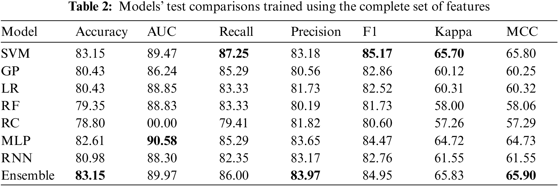
Fig. 5 compares both feature selection methods, χ2 Test and Importance Permutation, where the latter was computed using the best model from the previous experiments. Despite their distinct ordering, one can see that the top seven features are shared among the two rankings. The same goes for the bottom features, where both methods agree that they are mostly irrelevant to the task at hand. Following best intuition, the top seven features will be selected for the ablation study of feature selection [33].

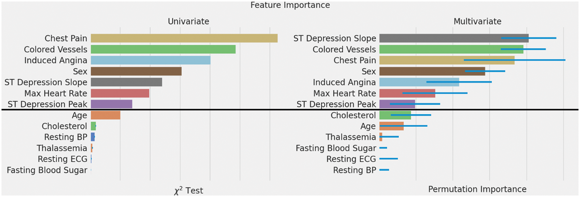
Figure 5: Feature importance rankings using two different methods

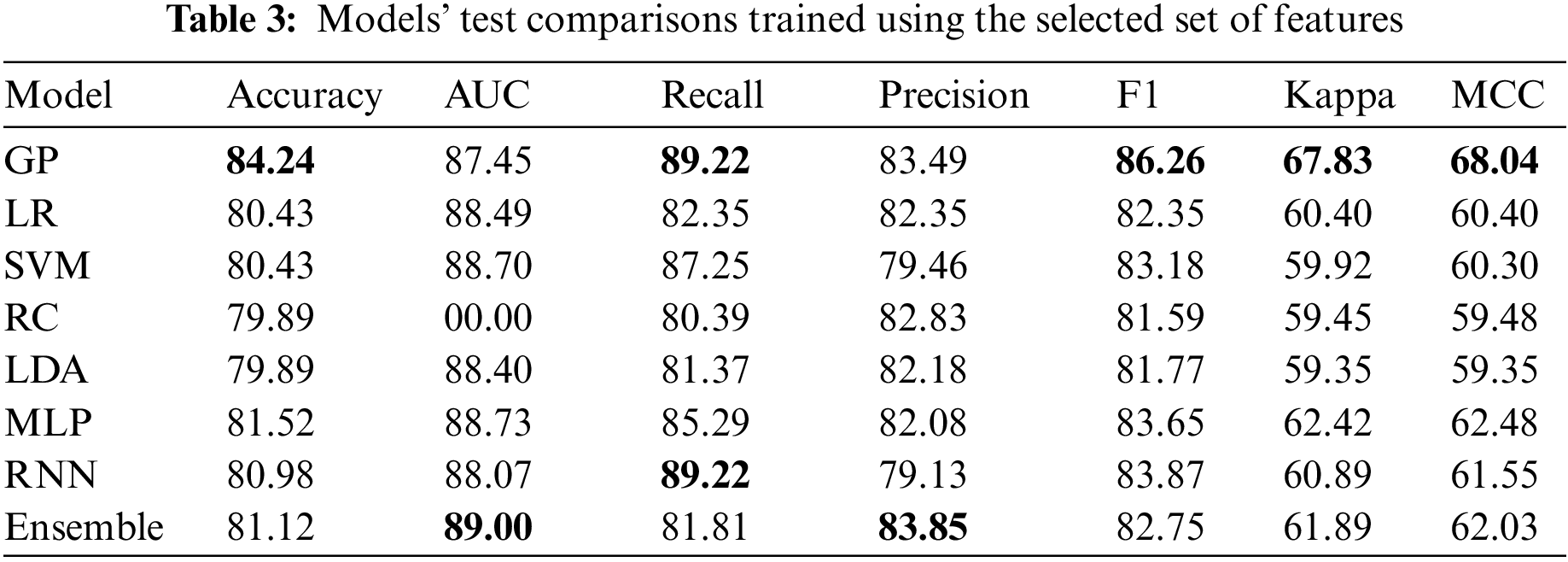
5.4 Results on the Selected Features

Table 3 shows that the best model for the selected features is the GP model. It is even better than all other models, including the deep learning and the ensemble model. More interestingly, the achieved accuracy is better than using the full features. Two things can explain this; the feature selection done on the best model on the complete feature set did its job ideally, and the GP model is more suitable when using fewer data under more uncertainty. The final observation is that the RNN model was not better in both experiments. However, its striking consistency despite using vastly different features demonstrates its robustness. This can mean that it has played a vital role in the model ensemble in Table 2.

5.5 Limitations and Future Work

The most significant limitation of this work is the non-sufficient data to draw statistically significant conclusions. This research can benefit greatly from more rich and diverse datasets publicly available for general use. To build on this work, one can collect more data and introduce new features that can improve the discriminative power of these classifiers. For example, the developed system can be used to collect anonymized data for similar future applications. Moreover, it might be interesting to predict the hardest available features using other more attainable information, extending the usability to a broader audience.

6  Conclusion

This research tackled the prediction problem of the UCI heart disease dataset in a feature-limited setting. It followed a proper data science workflow from data analysis and preprocessing to model building, training, and evaluation. In particular, this work trained multiple classical machine learning and deep learning models including a hybrid model of all the top performing models. Each model was tested under different hyperparameter configurations using a validation data split. Then, this paper applied feature selection and repeated the same process to get a model that uses only a subset of the features with competitive performance. This makes it easier for patients with limited access to benefit from the system while achieving an 84.24% accuracy, 89.22% Recall, and 83.49% Precision. As a result, this effort satisfied two critical goals of machine learning: interpretation and prediction.

Funding Statement: The authors received no specific funding for this study.

Conflicts of Interest: The authors declare that they have no conflicts of interest to report regarding the present study.

3The description of the models and evaluation metrics were omitted since they are not part of the contribution.

References

1. World Health Organization, “The top 10 causes of death,” 2020. [Online]. Available: https://www.who.int/news-room/fact-sheets/detail/the-top-10-causes-of-death. [Google Scholar]
2. E. J. Benjamin, P. Muntner, A. Alonso, M. S. Bittencourt, C. W. Callaway et al., “Heart disease and stroke statistics—2019 update: A report from the American heart association,” Circulation, vol. 139, no. 10, pp. 56–528, 2019. [Google Scholar]
3. S. Bashir, Z. S. Khan, F. H. Khan, A. Anjum and K. Bashir, “Improving heart disease prediction using feature selection approaches,” in Proc. of IBCAST, Islamabad, Pakistan, pp. 619–623, 2019. [Google Scholar]
4. A. H. Chen, S. Y. Huang, P. S. Hong, C. H. Cheng and E. J. Lin, “HDPS: Heart disease prediction system,” in 2011 Computing in Cardiology, IEEE, Hangzhou, China, pp. 557–560, 2011. [Google Scholar]
5. Center for Machine Learning and Intelligent Systems, “UCI machine learning repository,” Heart Disease Data Set, 1988. [Online]. Available: https://archive.ics.uci.edu/ml/datasets/heart+disease. [Google Scholar]
6. M. P. Alex and S. P. Shaji, “Prediction and diagnosis of heart disease patients using data mining technique,” in 2019 Int. Conf. on Communication and Signal Processing (ICCSP), Dalian, China, IEEE, pp. 848–852, 2019. [Google Scholar]
7. C. B. Gokulnath and S. P. Shantharajah, “An optimized feature selection based on genetic approach and support vector machine for heart disease,” Cluster Computing, vol. 22, no. S6, pp. 14777–14787, 2018. [Google Scholar]
8. A. U. Haq, J. P. Li, M. H. Memon, S. Nazir and R. Sun, “A hybrid intelligent system framework for the prediction of heart disease using machine learning algorithms,” Mobile Information Systems, vol. 2018, pp. 1–21, 2018. [Google Scholar]
9. I. Goodfellow, Y. Bengio and A. Courville, Deep Learning. San Francisco, CA, USA: MIT Press, pp. 1–26, 2016. [Google Scholar]
10. W. S. Noble, “What is a support vector machine?,” Nature Biotechnology, vol. 24, no. 12, pp. 1565–1567, 2006. [Google Scholar]
11. Y. Shen, Y. Li, H. -T. Zheng, B. Tang and M. Yang, “Enhancing ontology-driven diagnostic reasoning with a symptom-dependency-aware Naïve Bayes classifier,” BMC Bioinformatics, vol. 20, no. 1, pp. 1–14, 2019. [Google Scholar]
12. A. Gupta, L. Kumar, R. Jain and P. Nagrath, “Heart disease prediction using classification (Naive Bayes),” in Int. Conf. on Computing, Communications, and Cyber-Security, Springer, Singapore, pp. 561–573, 2020. [Google Scholar]
13. C. R. Shalizi, “Advanced Data Analysis from an Elementary Point of View,” Pittsburgh, Pennsylvania, USA: Cambridge University Press, pp. 234–260, 2019. [Online]. Available: https://www.stat.cmu.edu/~cshalizi/ADAfaEPoV/ADAfaEPoV.pdf. [Google Scholar]
14. Scikit-Learn, “Ridge regression and classification, linear models,” 2022. [Online]. Available: https://scikit-learn.org/stable/modules/linear_model.html#ridge-regression-and-classification. [Google Scholar]
15. G. J. McLachlan, “Logistic discrimination,” in Discriminant Analysis and Statistical Pattern Recognition, 1st ed., vol. 1. Queensland, Australia: John Wiley & Sons, pp. 255–282, 2005. [Google Scholar]
16. D. J. C. MacKay, “Introduction to Gaussian processes,” Cambridge, United Kingdom, 1998. [Online]. Available: https://citeseerx.ist.psu.edu/viewdoc/download?doi=10.1.1.81.1927&rep=rep1&type=pdf. [Google Scholar]
17. M. A. Friedl and C. E. Brodley, “Decision tree classification of land cover from remotely sensed data,” Remote Sensing of Environment, vol. 61, no. 3, pp. 399–409, 1997. [Google Scholar]
18. A. Liaw and M. Wiener, “Classification and regression by randomForest,” R News, vol. 2, pp. 18–22, 2002. [Google Scholar]
19. S. S. Yadav, S. M. Jadhav, S. Nagrale and N. Patil, “Application of machine learning for the detection of heart disease,” in ICIMI, Bangalore, India, pp. 165–172, 2020. [Google Scholar]
20. L. Medsker and L. C. Jain, “Recurrent neural networks: Design and applications,” in International Series on Computational Intelligence, 1st ed., vol. 1. Washington D.C., USA: CRC Press, pp. 1–10, 1999. [Google Scholar]
21. S. Mohan, C. Thirumalai and G. Srivastava, “Effective heart disease prediction using hybrid machine learning techniques,” IEEE Access, vol. 7, pp. 81542–81554, 2019. [Google Scholar]
22. R. Katarya and S. K. Meena, “Machine learning techniques for heart disease prediction: A comparative study and analysis,” Health and Technology, vol. 11, no. 1, pp. 87–97, 2020. [Google Scholar]
23. P. Dileep, K. N. Rao, P. Bodapati, S. Gokuruboyina, R. Peddi et al., “An automatic heart disease prediction using cluster-based bi-directional LSTM (C-BiLSTM) algorithm,” Neural Computing and Applications, vol. 34, no. 9, pp. 1–14, 2022. [Google Scholar]
24. Scikit-Learn, “Chi-squared statistic test feature selection,” 2022. [Online]. Available: https://scikit-learn.org/stable/modules/generated/sklearn.feature_selection.chi2.html. [Google Scholar]
25. M. Ali, “PyCaret: An open source, low-code machine learning library in python,” 2020. [Online]. Available: https://www.pycaret.org. [Google Scholar]
26. A. Paszke, S. Gross, F. Massa, A. Lerer, J. Bradbury et al., “PyTorch: An imperative style, high-performance deep learning library,” in Conf. on Neural Information Processing Systems, Vancouver, Canada, pp. 8024–8035, 2019. [Google Scholar]
27. E. Bisong, “Google Colaboratory,” in Building Machine Learning and Deep Learning Models on Google Cloud Platform, 1st ed., vol. 1. Berkeley, CA, USA: Apress, pp. 59–64, 2019. [Google Scholar]
28. C. R. Harris, K. J. Millman, S. J. Van Der Walt, R. Gommers, P. Virtanen et al., “Array programming with NumPy,” Nature, vol. 585, no. 7825, pp. 357–362, 2020. [Google Scholar]
29. The Pandas Development Team, “Pandas 1.4.2.,” 2022. [Online]. Available: https://pandas.pydata.org/. [Google Scholar]
30. F. Pedregosa, G. Varoquaux, A. Gramfort, V. Michel, B. Thirion et al., “Scikit-learn: Machine learning in python,” Journal of Machine Learning Research, vol. 12, pp. 2825–2830, 2011. [Google Scholar]
31. J. D. Hunter, “Matplotlib: A 2D graphics environment,” Computing in Science & Engineering, vol. 9, no. 3, pp. 90–95, 2007. [Google Scholar]
32. M. Waskom, “Seaborn: Statistical data visualization,” Journal of Open Source Software, vol. 6, no. 60, pp. 3021, 2021. [Google Scholar]
33. Scikit-Learn, “User guide to feature selection using scikit-learn,” 2022. [Online]. Available: https://scikit-learn.org/stable/modules/feature_selection.html. [Google Scholar]
Cite This Article
Copyright © 2023 The Author(s). Published by Tech Science Press.
This work is licensed under a Creative Commons Attribution 4.0 International License , which permits unrestricted use, distribution, and reproduction in any medium, provided the original work is properly cited.
Downloads
Citation Tools