Integrating WSN and Laser SLAM for Mobile Robot Indoor Localization

1  Introduction

Recently, both mobile robots and the internet of things (IoT) have been hot spots of research and can be used in many applications [1]. The intelligent mobile robot can be thought of as an autonomous mobile terminal in the WSN while the sensors or other devices are the static terminals. It’s already common that mobile robots serve human beings in many areas, for instance, there are many commercial service robots used for transporting goods in industrial parks, factory workshops, hotels, restaurants, and hospitals, especially during the COVID-19 epidemic time [2]. The premise for robots to perform these tasks is that they can navigate and plan paths autonomously [3]. Before the navigation, the mobile robot needs to achieve its pose which includes position coordinates and orientation on a two dimensional plane. Given the initial pose and a target position, the following navigation process will be a relatively mature work. Therefore, localization task is vital and meaningful in mobile robotics research.

In an outdoor environment, the global positioning system (GPS) is the most popular and widely used location technology in the world [4]. Due to the absence of GPS signal in the indoor environment, many other signals are proposed to solve this problem, for instance, WiFi [5], ultrasonic, radio frequency identification (RFID) [6], ultrawide-band (UWB) [7] and WSN [8]. RSSI is usually used to calculate the approximate distance between the receiver and the signal transmitter [9]. However, these methods can only provide basic and rough localization information. The mobile robot still cannot know where is the free area or obstacle, thus cannot navigate or walk freely in the environment. Another route is focused on the 2D laser rangefinder or Lidar which can be used to achieve the 2D metric information and map the environment around the mobile robot. In addition, the metric map is suitable and effective for path planning. A 2D probabilistic occupancy grid map is built firstly using a technique called SLAM, then the mobile robot performs the localization task according to the constructed map and Monte Carlo localization method (MCL) [10]. However, when the mobile robot moves to a geometrically similar area, the 2D laser sensor gets the same data from its surroundings and the localization task becomes very difficult [11].

To solve the above localization problem in a geometrically similar indoor environment, such as a long corridor, this work provides an alternative scheme by combining the WSN and laser SLAM techniques. Firstly, we build a hybrid map using the two techniques. Then, we utilize a coarse-to-fine paradigm that uses signal retrieval to get a coarse position candidate. Lastly, the laser scanning data are used to achieve a fine localization pose. The whole framework of the mapping and localization system is depicted in Fig. 1. The main contributions of this work are as follows:

•   A hybrid map consisted of the fingerprints of signal values and an occupancy grid map is built when the mobile robot moves in a geometrically similar environment. The coordinates of the signal nodes are determined based on the laser SLAM mapping progress.

•   The joint initialization of the global localization. The mobile robot achieves the coarse position without orientation according to the RSSI retrieval and then moves a short distance to decide the orientation. The fine localization task is done by using the laser scanning data and the improved MCL method.

•   An improved resampling strategy is used to detect the robot kidnapping incident. RSSI values and the fixed time interval are considered as the references. Experimental results show that our proposed approach is efficient and achieves a 97.0% successful localization rate within one meter moving distance while traditional MCL methods always fail. In addition, the robot can rapidly recover its pose from a kidnapped incident.

Figure 1: Framework of the mapping and localization system

This paper is organized as follows. The related work of laser-SLAM and localization, and WSN-assisted localization are discussed in Section 2. A proposed methodology is presented in Section 3, which includes building an occupancy grid map, RSSI-distance fingerprint, building a hybrid map and coarse-to-fine localization. The experiment and discussion are described in Section 4. Finally, Section 5 gives the conclusion.

2  Related Work

2.1 Laser SLAM and Localization

Laser SLAM is mainly used for constructing a grip map of the environment where the mobile robot performs tasks. Due to the high costs, 3D laser Lidar is usually used for outdoor self-driving [12] or indoor 3D reconstruction [13]. In an indoor environment, most of the surroundings are structured scenes, mobile robot only needs to know which areas can pass through for navigation. Therefore, the 2D laser Lidar is enough for the purpose of building a two-dimensional probability occupancy grid map. This map is used for the following path plan. The most famous works of the 2D laser Lidar SLAM are Gmapping [14] and Cartographer [15]. The former is a filter-based scheme and the latter is a graph optimization scheme. In addition, there are other options such as hector SLAM [16] and Karto SLAM [17].

Localization solves the question ‘Where am I’ and includes three cases which are global localization, pose tracking (local localization) and the kidnapped robot problem [18]. Global localization means the robot needs to know its pose when it wakes up anywhere on a given map. Kalman filter and its extended versions are mainly used for pose tracking, not suitable for global localization and robot kidnapped problems [19,20]. On the contrary, particle filter approaches can solve the whole cases [21]. Monte Carlo localization methods use particles to simulate arbitrary distribution. More importantly, they are suitable to deal with nonlinear and non-gaussian problems. However, for those geometrically similar environments, the MCL method will fail.

2.2 WSN-Assisted Localization

WSNs have been applied in the field of localization which mainly depends on RSSI [22], such as search and rescue environment [23], and underwater scenes [24]. Generally, the geometric and fingerprint approaches are commonly used in RSS indoor localization systems. Due to the non-line-of-sight (NLOS), the geometric approach implements easily but has low position accuracy [25]. Differently, the fingerprint method requires only the collection of RSS values at several fixed locations. The signal fingerprint is usually performed in an offline surveying phase and followed by an online querying phase [26]. In the offline phase, a database is formed by collecting several location fingerprints. In the online phase, the mobile robot or agent collects several RSS values to calculate the approximate position.

However, due to the environmental impacts, the measured RSSI value is time-varying and unreliable [27]. Consequently, the mobile robot localization only based on the WSN method cannot achieve an accurate location. More seriously, the orientation of the mobile robot cannot be determined and the RSSI information is not enough for obstacle avoidance. The combination of WSN and SLAM is a new trend, especially in the field of mobile robotics. In literature [28,29], the authors combine the two techniques to realize an accurate pose estimating error. However, they only did the SLAM process, not the re-localization in the environment given a known map. In addition, the map points were some simulated sparse features which are not suitable for path planning and navigation tasks [30]. Gives a result of the fusion of WiFi, IMU and SLAM. The result is only thought of as an odometry measurement, still not a re-localization task according to a previously built map. Different from all these works, our proposed approach combines the laser-based SLAM and the RSSI techniques to build an occupancy grid map. Based on the known map, the autonomous mobile robot can realize a better localization result.

3  Proposed Methodology

3.1 Build an Occupancy Grid Map

In the map building phase, the mobile robot utilizes the SLAM technique to solve a contradictory problem. The SLAM is a process that a mobile robot perceives an unknown environment and constructs a map. The mobile robot needs to concurrently estimate the robot pose and the environmental structures. In general, a 2D laser-based SLAM mapping system needs odometry to estimate the moving process and a laser rangefinder to estimate the measurement process.

Fig. 2 shows a diagram of the mobile robot motion model based on odometry which is an encoder attached to each wheel of the mobile robot. Suppose the poses of the robot at time t−1 and t are xt−1=(xt−1,yt−1,θt−1) and xt=(xt,yt,θt), respectively. The black cycle on the lower left represents the position of the mobile robot at time t−1 and the black solid arrow means the orientation. Similarly, the upper right part means that of time t. The displacement of the robot from time t−1 to time t can be decomposed into one translation (δtrans) and two rotations (δrot1 and δrot2).

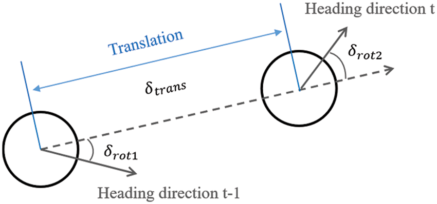
Figure 2: Diagram of the mobile robot motion model

If the influence of error is not considered, then the translation and rotations can be computed from Eq. (1).

{δrot1=atan2(yt−yt−1,xt−xt−1)−θt−1δtrans=(xt−xt−1)2+(yt−yt−1)2δrot2=θt−θt−1−δ^rot1(1)

However, due to the drift and slip of wheels, there is no fixed coordinate transformation between the coordinates used by the odometer in the mobile robot and the coordinates of the physical world. The difference between the real value and the ideal value can be obtained by sampling, as Eq. (2) shows:

{δ^rot1=δrot1−sample(α1δrot12+α2δtrans2)δ^trans=δtrans−sample(α3δtrans2+α4δrot12+α4δrot22)δ^rot2=δrot2−sample(α1δrot22+α2δtrans2)(2)

where the variables α1, α2, α3, and α4 are the specific parameters that specify the robot motion noise. δ^rot1, δ^rot2, and δ^trans are the estimated results. Then, taking all these information together, the odometry-based probabilistic motion model from time t−1 to t can be defined as Eq. (3):

(xtytθt)=(xt−1yt−1θt−1)+(δ^transcos⁡(θ+δ^rot1)δ^transsin⁡(θ+δ^rot1)δ^rot1+δ^rot2)(3)

The measurement function usually utilizes the likelihood field model instead of beam rangefinder model. The reason is that the latter one lacks of smoothness. Suppose the (xk,sens,yk,sens)T represents the position of the sensor local coordinate system fixedly connected with the mobile robot and θk,sens means the angle of sensor beam relative to robot the heading direction. The endpoint coordinates of the measurement ztk can be mapped to the global coordinate system through triangular transformation, as Eq. (4) shows.

(xztkyztk)=(xtyt)+(cos⁡θsin⁡θ−sin⁡θcos⁡θ)(xk,sensyk,sens)+ztk(cos⁡(θ+θk,sens)sin⁡(θ+θk,sens))(4)

The measurement probability q calculated by the likelihood domain is as bellow:

{dist=minx′,y′⁡{(xztk−x′)2+(yztk−y′)2|⟨x′,y′⟩occupied in m}q=q⋅(zhit⋅prob(dist,σhit)+zrandomzmax(5)

where (x′,y′) is the position of the obstacle in the map system, zhit is the normal measured distance, zrandom is the random measured distance and zmax is the maximum value of the sensor. Given the known map and observation values, the localization problem is easy to solve. Similarly, given the pose and observation of the robot, it is easy to build a map. However, the mapping process without a known pose which also is named SLAM is difficult. The reason is that the mobile robot needs to concurrently estimate its pose and build a metric map. The SLAM technique can be thought of as a state estimation problem which jointly estimates the poses and observations. A diagram of SLAM process is shown in Fig. 3. The hexagonal star with a solid black line indicates the position of the real observation landmark and the triangle with a red solid line represents the real pose of the robot. In contrast, the hexagonal star with a dashed black line indicates the position of the estimated observation landmark and the triangle with a red dashed line represents the estimated pose of the robot. Due to the measurement errors of the odometer and observation sensor, it is difficult to obtain accurate values, so the error can only be reduced as much as possible.

Figure 3: SLAM or state estimation

The probabilistic occupancy grid map can be thought of as a combination of many basic grid cells. The grid cells are the discretization of a place and the mathematical equation can be described as follows:

p(m|z1:t,x1:t)=Πip(mi|z1:t,x1:t)(6)

where m is the map to be built and mi is the i-th cell of the map. The logarithmic probability expression (7) is to avoid the numerical instability near 0 and 1.

{p(mi|z1:t,x1:t)=1−11+exp⁡{lt,i}lt,i=log⁡p(mi|z1:t,x1:t)1−p(mi|z1:t,x1:t)(7)

where lt,i is the expression of logarithmic occupancy probability. The SLAM process can be expressed as:

p(x1:t,m|z1:t,u1:t)=p(x1:t|z1:t,u1:t)p(m|x1:t,z1:t,u1:t)=p(m|x1:t,z1:t)p(x1:t|z1:t,u1:t)(8)

3.2 RSSI-Distance Fingerprint

The database of RSSI-distance fingerprints needs to be created before the localization and navigation process. Fig. 4 shows the diagram of the localization which includes reference signal points and a mobile robot mounted with a signal receiver. The mobile robot collects signal information in different positions and saves them into a database.

Figure 4: The diagram of RSSI-based localization

In Fig. 4, the blue marks are reference signal nodes which are also called signal beacons or points in other literatures. Although the names are different, the essential effects are the same. They are usually placed in the indoor environment in advance and given the known coordinates by manual calibration. The locations of all reference signal nodes could be denoted as LOCRN and were shown in the following formula.

LOCRN=[x1y1,x2y2,⋯xiyi,⋯xnyn]T(9)

where (xi,yi) means the i-th coordinates of the reference signal node and n is the total number of reference signal nodes.

The red dot represents a mobile robot that carries a signal receiving node. Theoretically, in all areas covered by the reference node signals, the receiver node can receive an RSSI value from each reference signal node. Consequently, sampling signal strengths at several fixed points can be thought of as collecting signal fingerprints. The black dots in Fig. 4 denote the fixed sampling points. In each sampling point or position, the receiving RSSI values can be denoted as a signal vector or fingerprint FPi, as formula 10 shows.

FPi=(rssi1rssi2⋯rssij⋯rssin)(10)

where rssij is the receiving signal strength value from the j-th signal node to the i-th sampling position. In the i-th sampling position, the receiver node can achieve n RSSI values if the n signal nodes are distributed within a visual range.

The fingerprint database consists of m vectors which are RSS values combined and collected from sampling points, as formula 11 shows.

FP=[rss11rss12⋯rss1nrss21rss22⋯rss2n⋮⋮⋮⋮rssm1rssm2⋯rssmn](11)

The next work is to achieve the relationship between the receiving signal strength and the distance information. Given the relationship and the RSSI value, the distance from the i-th sampling point to each reference signal node can be computed. Similarly, the position of the i-th sampling point can be a trilateral theorem or the least square value by solving nonlinear equations [31]. Therefore, the key to the problem is how to obtain the distance according to the receiving signal strength. A classical path-loss equation [32] for the corridor or open space scene in this work is defined as follows.

{RSSIdi(dBm)=RSSId0(dBm)−[10×α×log10⁡(did0)]+δdi=d0×10RSSId0(dBm)−RSSIdi(dBm)+δ10×α(12)

where di is the distance from the reference signal node to the i-th sampling point. d0 is usually set to 1 as a reference value. RSSIdi is the mean RSSI value that is collected at the i-th sampling point, similarly with the RSSId0. δ is the measurement noise and α is the signal attenuation index.

After knowing the distance from each sampling point to each reference point, it is easy to calculate the position coordinates of the sampling point LOCsi, as follows:

{dsi−RN=(dsi1,dsi2,⋯,dsinLOCsi=(xsi,ysi)(13)

3.3 Build a Hybrid Map

Different from the traditional practice in the field of communication, we do not mark the coordinates of the reference signal nodes in advance. We utilize the laser-based SLAM to construct an occupancy grid map, in the meanwhile, mark the position of the reference signal node on the map according to the path-loss equation and relative calculation formulas. The purpose is to convert the coordinates of RNs into the coordinate system of the mobile robot and the world coordinate system. Then, the coordinates of the RNs in the map can be represented as formula 14:

MapRN=[mx1my1,mx2my2,⋯,mxnmyn]T(14)

where (mxi,myi) is the coordinates of the i-th reference signal node in the grid map as Fig. 5 shows.

Figure 5: The diagram of building a hybrid map

In Fig. 5, each of the RNs is placed on the wall near the door frame which has a corner and is easy to identify. After building the grid map, the coordinates of the RNs are marked manually according to the world coordinate.

3.4 Coarse-to-Fine Localization

Given a known map, the localization mode uses a coarse-to-fine paradigm to achieve the mobile robot pose. Instead of uniformly sampling particles from the whole occupancy grid map, we bias the region which recommended by the RSSI retrieval result. Due to the infinity of continuous space, the sampling points cannot cover all areas in the indoor environment. Therefore, when the mobile robot moves in the coverage area, the estimation position can be computed according to Eq. (15).

{(xest−x1)2+(yest−y1)2=d12(xest−x2)2+(yest−y2)2=d22⋯(xest−xn)2+(yest−yn)2=dn2(15)

However, the above computation equation is effective only under ideal conditions. In practice, the distance di between the estimation position and a reference node can not be obtained directly. To this end, we use the K Nearest Neighbor (KNN) algorithm to achieve the most likely position of the mobile robot relative to the sampling points [33]. Obviously, the mobile robot is located in a subarea between the two or adjacent reference signal nodes with the highest RSSI values, like the green area in Fig. 6a.

d(rssestk,rsssi)=∑j=1m(rssiestj−rssiij)2(16)

where m is the number of RFs which have high RSSI values relative to the i-th sampling point. k is the number of sampling points near the position that needs to be estimated.

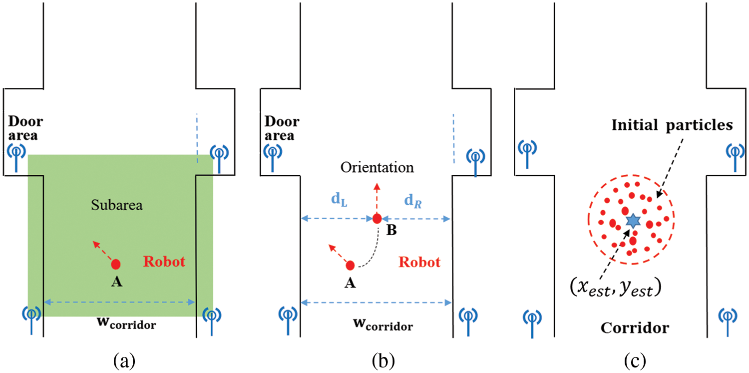
Figure 6: Coarse localization diagram. (a) Subarea determination. (b) Slightly adjustment to obtain orientation. (c) Particles initialization

The position of the mobile robot can be coarsely determined by using RSSI information, however, the orientation of the mobile robot cannot be determined. To this end, our proposed strategy is that the mobile robot moves a short distance and detects the signal difference. As Fig. 6b shows, the mobile robot moves from position A to position B to obtain a best perspective like our previous work [11]. If the RSSI value in the estimation position B relative to RN-i increases, then the orientation is toward the RN-i, otherwise, toward the opposite direction.

After knowing the initial position and orientation of the mobile robot, the following task is to get a fine localization using an improved particle filter algorithm. In the initialization of the global localization step, the particles are scattered evenly in a circular area as Fig. 6c shows and the representation is shown in Eq. (17):

(x−xest)2+(y−yest)2=R2(17)

where R is the radius of the circular and the weights of the particles are equal to 1/N where N is the number of particles. In this work, the weights are given by a gaussian distribution function as Eq. (18):

winitial=P((x,y);u,Σ)=12πΣ12exp⁡(−12(x−xest)TΣ−1(y−yest))=12πσxσyexp⁡(−((x−xest)2σx22+(y−yest)2σy22))(18)

where (xest,yest) is the estimated position of the robot. The orientations of the particles are parallel to the corridor, so random generation is not required. Fig. 7 shows the particles with different weights.

Figure 7: Particles with different initialized weights

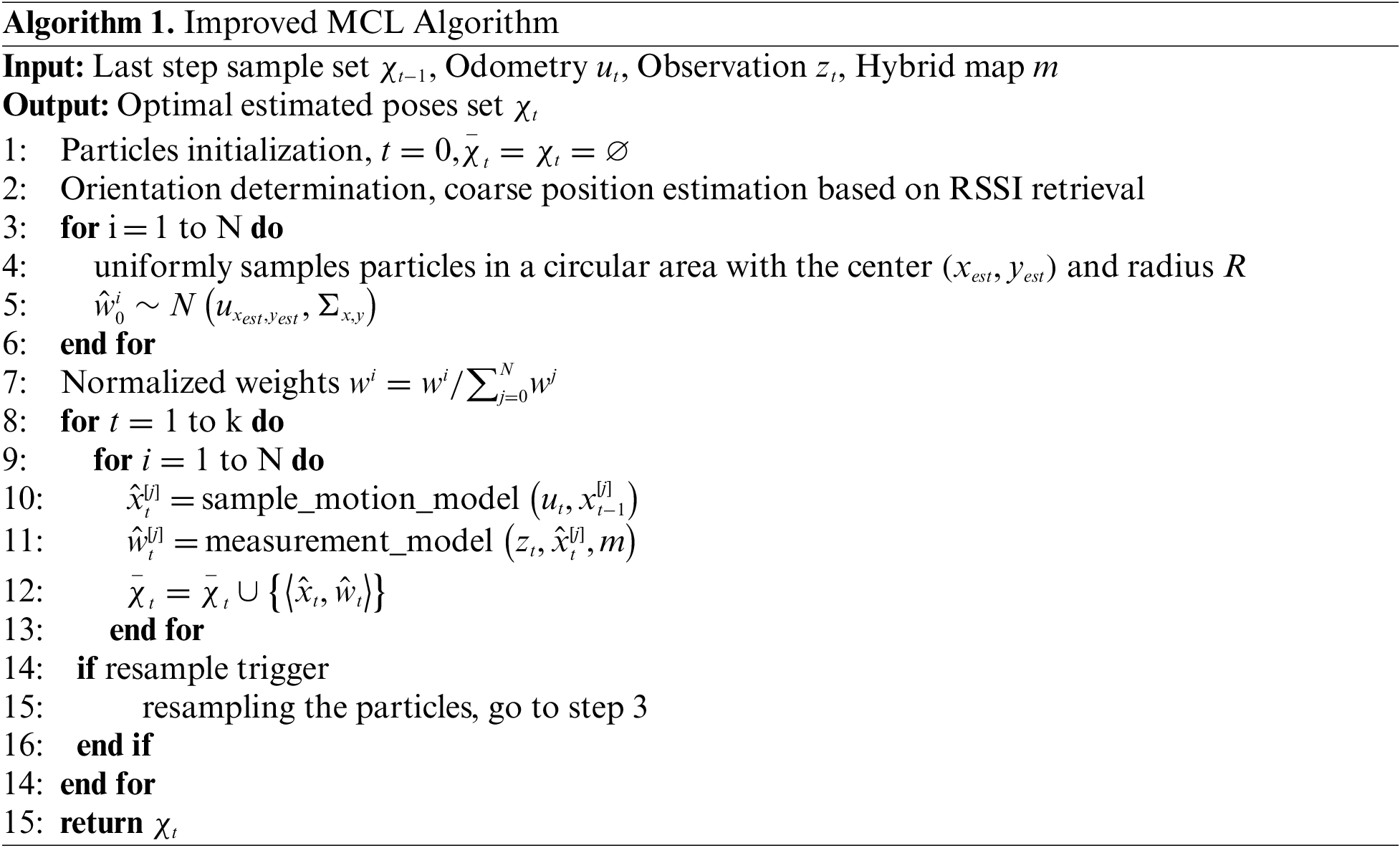
A detailed algorithm is described in Algorithm 1. The observation data includes the laser scanning distances and the RSSI values. Resampling trigger can be set to a fixed time interval. Different from many other resampling schemes that simply replicate the particles with high weights and lose the particle diversity [34], our proposed approach resamples particles according to the RSSI retrieval result after a fixed time interval. Consequently, we do not need to worry about losing particle diversity or spending time on complex resampling algorithms.

4  Experiment and Discussion

Our experimental mobile robot is a modified two-wheel differential driving vehicle shown in Fig. 8a. A RPLIDAR A2 laser Lidar (SLAMTEC company, China) which has a 360-degree rotation range and an effective measurement radius of 8 to 10 meters in practice. In addition, the microcomputer with 1.5 GHz ARM Cotex-A72 CPU and 8GB RAM. The reference signal nodes and the signal receiver node use the CC2530 module (Texas Instruments, USA) which is based on the ZigBee protocol and IEEE 802.15.4 standard.

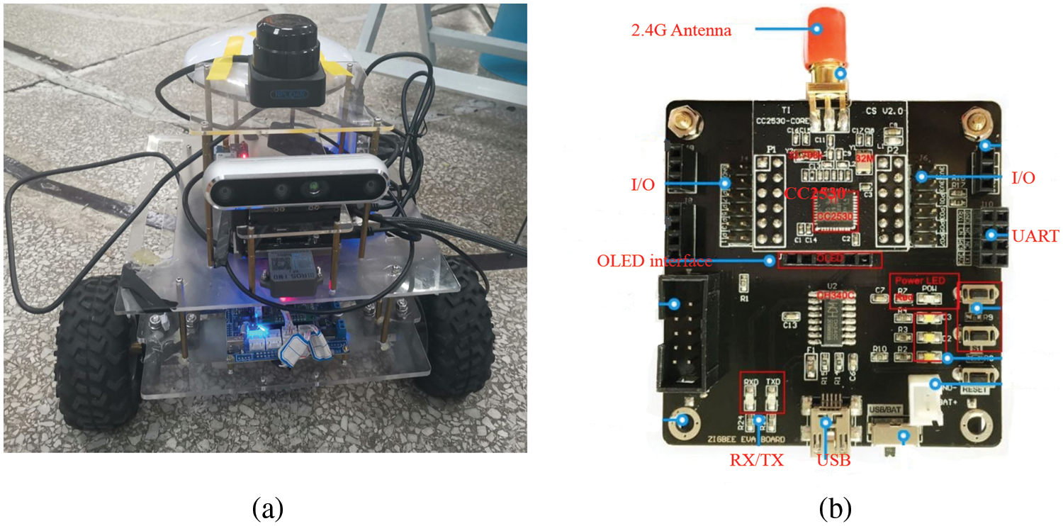
Figure 8: Experimental setup. (a) The mobile robot platform. (b) CC2530 module

The occupancy grid map is built by using the cartographer SLAM method. The experimental environment is a long corridor with many symmetrical and similar areas inside a student dormitory as shown in Fig. 9. It is obvious that the mobile robot will fail to locate itself because of the similarity of laser scanning data. The length of the corridor is 43.50 m and the width in the non-door area is 1.85 m. We put 10 reference signal nodes on one side of the corridor and paste them on each door. 26 positions are chosen as the sampling points to collect the RSSI fingerprints.

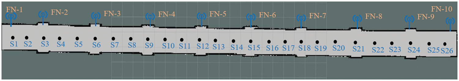
Figure 9: RF nodes and sampling points in the occupancy grid map of the environment

4.1 Global Localization

In the global localization experiment, we sampled 27 positions in the corridor and most of them were between two adjacent reference sampling points as shown in the black star signs in Fig. 10. The ground truth of the signed positions and the distances were measured manually using a tape ruler. In addition, the whole area was divided into 9 subareas as shown in the green rounded rectangles in Fig. 10. The subarea was between two adjacent reference signal nodes.

Figure 10: Diagram of the test points distribution

The first experiment was the coarse localization of the fingerprint retrieval method using RSSI values and the KNN algorithm. The mobile robot mounted with a signal receiver module was placed on the target sampling position to collect RSSI values and compute the coordinates. 10 times tests with random robot heading directions in each test position were conducted. The total number of tests was 270 and we recorded the experimental data to obtain some statistical results. If the computed coordinates of the test position fell into the relative subarea, we thought it was a correct subarea localization. Due to the existence of various errors and noises, it was impossible to achieve an absolutely accurate positioning coordinate. Therefore, we recorded the number of positioning errors within 1.0 meters and 2.0 meters, respectively. Table 1 shows the coarse localization result using this method.

The detailed error values from the subarea between FN6 and FN7 as shown in Fig. 11.

Figure 11: Errors of the 10 times results in each test position of a subarea

From left to right, the three estimated test positions E16, E17, and E18 were represented by the black rectangle, red-filled circle, and blue triangle, respectively. At each test position, we recorded the absolute value of the difference between the estimated coordinates and the real position coordinates. Although there was a random error in each measurement, the mean error of all the 30 tests was 0.98 meters which was less than 1 meter and was within an acceptable range.

The second experiment consisted of two separate parts. One of them used the traditional AMCL method to get a global localization task without a known initial pose, the other utilized our proposed approach and strategy to obtain an initialization based on the RSSI retrieval result. Both the two parts aimed to get a fine localization pose. Figs. 12 and 13 are the results of the traditional MCL method and our proposed method, respectively.

Figure 12: Global localization process of traditional AMCL. (a) Initialization of the particles. (b) 12 iterations. (c) 25 iterations. (d) 57 iterations. (e) 79 iterations with a wrong pose

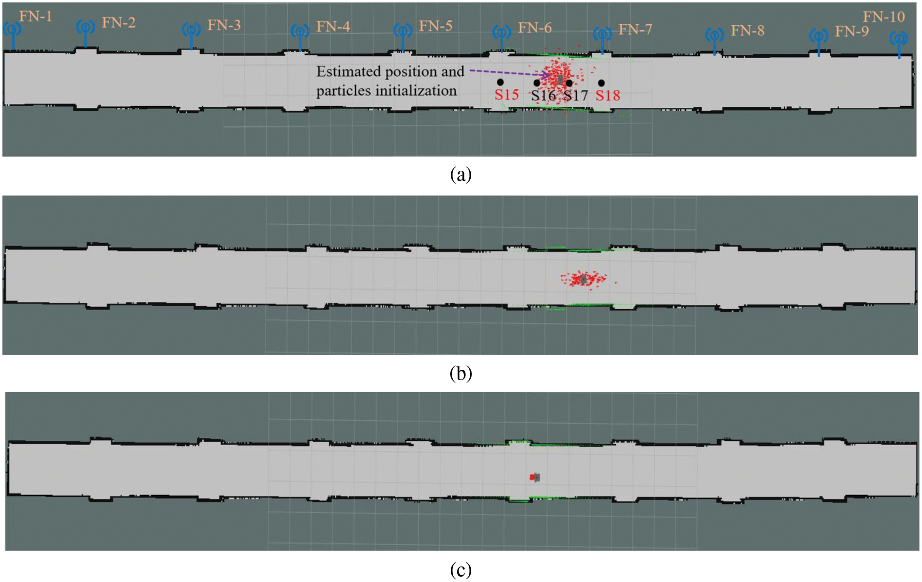
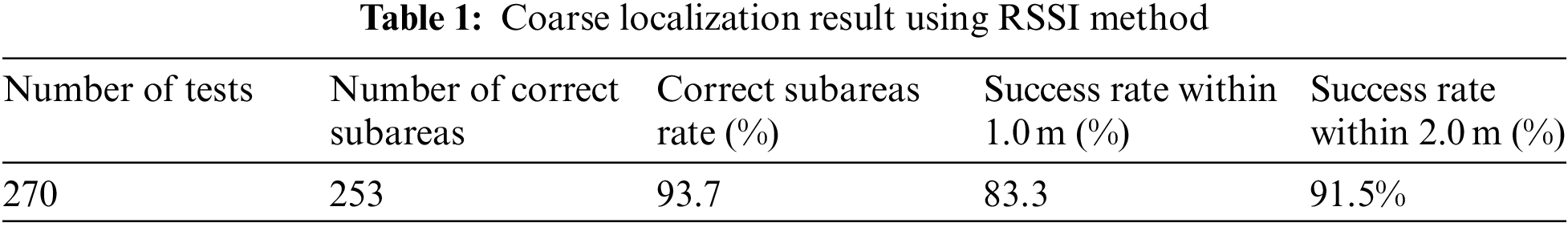
Figure 13: Global localization results of the proposed method. (a) Initialization of the particles. (b) Particle distribution after moving a short distance. (c) Successful localization when particles converged

In Fig. 12a, the mobile robot was placed manually at position E17, then a global localization task was performed. Due to the unknown initial pose of the mobile robot, the particles were scattered evenly on the whole map. The number of particles was usually proportional to the area of the map. In other words, the larger the map, the more particles were required. The mobile robot was controlled to move to the right side of the corridor. Fig. 12b shows a result after 12 iterations (we uniformly called the number of resampling as the number of iterations). The particles gradually clustered into many clusters. Fig. 12c demonstrates the process after 25 iterations. In Fig. 12d, we find that the cluster is 3 and the mobile robot has moved closer to the end of the corridor. To obtain a single cluster, we controlled the mobile robot moving reversely and Fig. 12e shows the final state. Unfortunately, this pose is not the real pose in the corridor. More experiments have verified the failure of traditional methods in similar environments.

Different from the traditional AMCL method, our proposed strategy gets a coarse localization result from fingerprint retrieval according to the RSSI values. The achieved position was within an error range and did not have orientation information. The orientation was decided according to the strategy described in Section 3.4 and Fig. 6b. After a slight adjustment to get the orientation information from position E17, the particle initialization was shown in Fig. 13a. Obviously the number of particles was less than that of the traditional method.

To get a fine localization result, the mobile robot should move a short distance and the particles would converge to a single cluster. Fig. 13b shows the particles in the longitudinal direction of the corridor gradually become narrower. This phenomenon indicates that the lateral error is small because the width of the corridor is within the scanning radius of the laser sensor. Similarly, the longitudinal error is slightly larger than the lateral error which is due to the long distance of the corridor. When the mobile robot moved to the position close to the door area, the uncertainty was less, as shown in Fig. 13c, and a fine localization process ended. After that, the task is the pose tracking which also is called local localization.

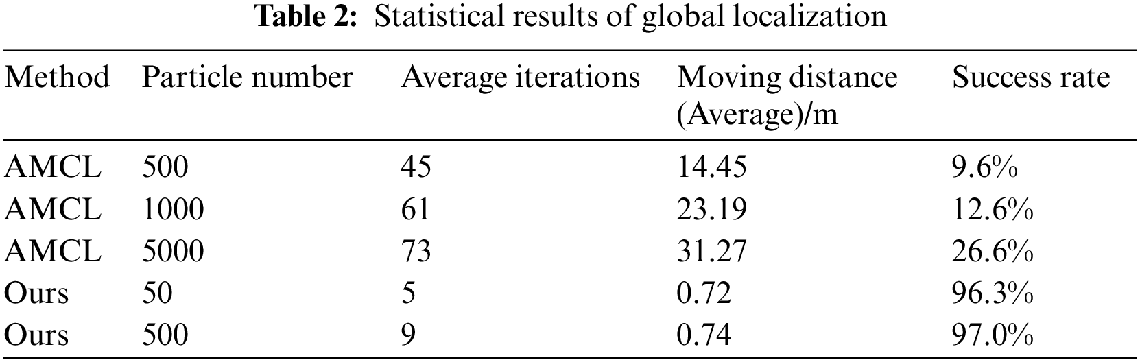
We placed the mobile robot at every tested position to perform global localization tasks and conducted it 10 times at each position. The average results of the localization process are shown in Table 2. When using the traditional AMCL method, we controlled the mobile robot moving along the corridor till the particles converge into a single cluster. If the mobile robot did not converge after reaching the end of the corridor, it would continue to move in the opposite direction. The results show that the traditional method has a low global localization success rate even though the number of particles increases. In contrast, our proposed method can achieve a high success localization rate with few particles.

4.2 Recovery from Robot Kidnapping

When a mobile robot was kidnapped from one position to another position, we tested the traditional method and our proposed approach, respectively. If the constructed map had salient geometrical or structural features that were extracted by laser scanning data, the mobile robot usually could recover its pose after a period of adjustment using the traditional AMCL method. Nevertheless, as shown in Fig. 14, many areas are geometrically similar when using only laser scanning data. Neither 2D laser rangefinder nor 3D laser Lidar could distinguish the highly similar or symmetrical areas in the corridor.

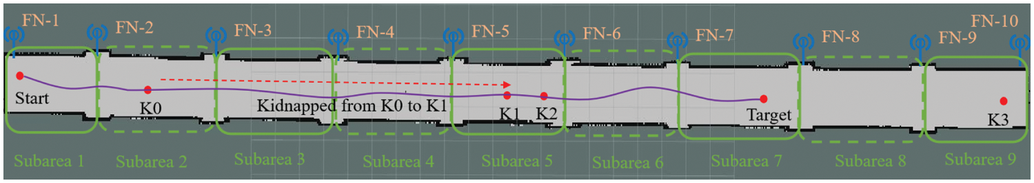
Figure 14: Diagram of the kidnapped robot problem

In this experiment, we placed the mobile robot on the left side of the corridor and gave its initial pose manually. The navigation task was moving from the start position to the target position on the right side of the corridor. As shown in Fig. 14, the start position and target position are fell into subarea 1 and subarea 7, respectively. In Fig. 14 the purple line is the planned path using the navigation package and the robot will reach the target position smoothly if without accident. When the robot moved to position K0, we kidnapped the robot and placed it at position K1 where the scanning data of the surrounding area was similar to that of K0. The traditional AMCL method could not find the change and the mobile robot continued to move forward until it reached position K3. Unfortunately, the mobile robot could not recover its pose from this kidnapped accident though the surroundings at position K3 was different from the target position.

Another experiment repeated the above process but used our proposed strategy. When the mobile robot was kidnapped from K0 to K1, the robot did not immediately notice the change but moved forward to the target position. Due to the resampling strategy of our proposed method, the mobile robot would resample the particles according to the RSSI values and signal fingerprint retrieval after a fixed time interval. Then, the mobile robot would find itself falling into subarea 5, not subarea 2 or subarea 3. Theoretically, the signal receiving values could be confirmed by multiple times tests and computations which confirmed the kidnapped robot accident with a larger probability.

Two error variation processes using different methods when the kidnapped mobile robot problem occurred are shown in Fig. 15. The abscissa is the time interval and the ordinate is the positioning error. Before time zero, the mobile robot worked normally and moved from one position to another. We thought the time when the robot was kidnapped as time zero. Fig. 15a shows that the traditional AMCL method could not find the changes before and after the kidnapping accident though the real error kept at about 14.85 meters. The robot would eventually be lost in the long corridor environment and was unable to recover its true position and orientation. In contrast, as shown in Fig. 15b, our proposed method found the change after a fixed time interval (empirically set to 8 s which was a resampling strategy) and soon recovered its pose in the real world.

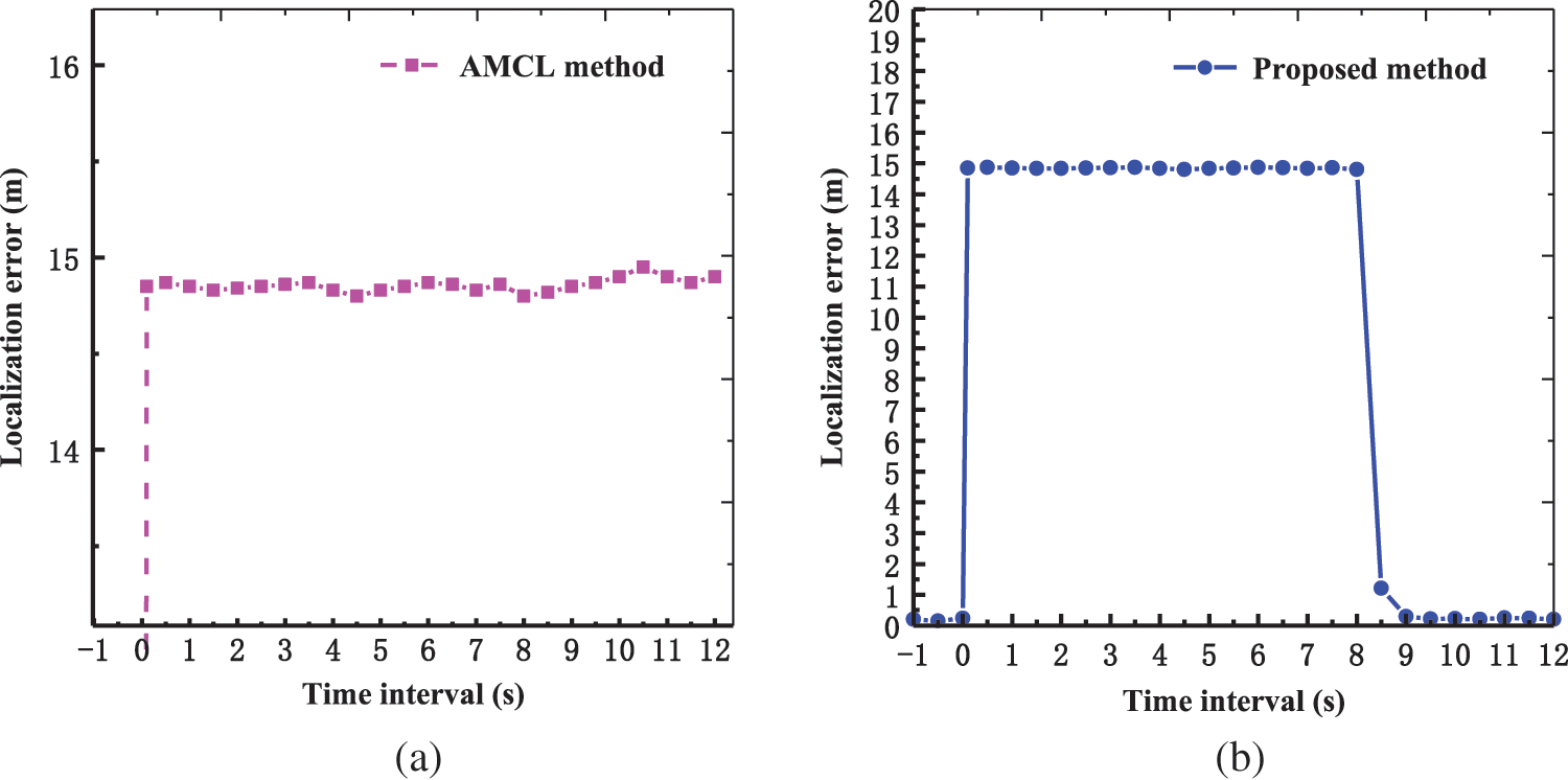
Figure 15: Recovery from the kidnapped robot problem. (a) Error variation of AMCL method. (b) Error variation of the proposed method

5  Conclusion

In this work, we propose a novel approach that combines WSN and laser Lidar-based SLAM to realize a robust and accurate localization for an autonomous mobile robot. A hybrid map with occupancy grid cells and RSSI values is built in the mapping stage. Then, the mobile robot accomplishes the localization task by using a coarse-to-fine paradigm. We use the newly captured RSSI values to compare with the sampling points in the map building stage and calculate the coarse position of the mobile robot. However, the position is not accurate and has no orientation information. Our proposed strategy can rapidly get a basic orientation of the mobile robot. Fine localization is realized by using an improved MCL approach. Experimental results demonstrate that our method is effective and robust for global localization. The localization success rate reaches 97.0% and the average moving distance is only 0.74 meters, while the traditional method always fails. In addition, the method also works well when the mobile robot is kidnapped to another position in the environment.

Although this work can deal with the localization problem in the geometrically similar environment, external signal nodes need to place at fixed positions in advance. In the future work, we will try other technical means to assist SLAM localization solution, such as camera and image processing. Without considering the external signal node cost, this scheme is very effective and can be applied to more indoor environments, such as stations, factories and libraries. In addition, this work can be extended to an outdoor environment like forest or tunnel scenes by using 3D Lidar SLAM and WSN techniques.

Funding Statement: This paper is funded by the Key Laboratory Foundation of Guizhou Province Universities (QJJ [2002] No. 059). The work is also supported by the Natural Science Research Project of Guizhou Province Education Department (Grant Number KY [2017]023, Guizhou Mountain Intelligent Agricultural Engineering Research Center), Doctoral Fund Research Project of Zunyi Normal University (Grant Number ZS BS [2016]01, Aerial Photography Test and Application of Karst Mountain Topography).

Conflicts of Interest: The authors declare that they have no conflicts of interest to report regarding the present study.

References

1. C. M. J. M. D. Junior, S. P. P. Da Silva, R. V. M. Da Nobrega, A. C. S. Barros, A. K. Sangaiah et al., “A new approach for mobile robot localization based on an online IoT system,” Future Generation Computer Systems, vol. 100, pp. 859–881, 2019. [Google Scholar]
2. X. V. Wang and L. Wang, “A literature survey of the robotic technologies during the COVID-19 pandemic,” Journal of Manufacturing Systems, vol. 60, pp. 823–836, 2021. [Google Scholar]
3. B. K. Patle, G. Babu L, A. Pandey, D. R. K. Parhi and A. Jagadeesh, “A review: On path planning strategies for navigation of mobile robot,” Defence Technology, vol. 15, no. 4, pp. 582–606, 2019. [Google Scholar]
4. E. Zhang and N. Masoud, “Increasing GPS localization accuracy with reinforcement learning,” IEEE Transactions on Intelligent Transportation Systems, vol. 22, no. 5, pp. 2615–2626, 2020. [Google Scholar]
5. B. Huang, R. Yang, B. Jia, W. Li and G. Mao, “A theoretical analysis on sampling size in WiFi fingerprint-based localization,” IEEE Transactions on Vehicular Technology, vol. 70, no. 4, pp. 3599–3608, 2021. [Google Scholar]
6. A. Motroni, A. Buffi and P. Nepa, “A survey on indoor vehicle localization through RFID technology,” IEEE Access, vol. 9, pp. 17921–17942, 2021. [Google Scholar]
7. L. Barbieri, M. Brambilla, A. Trabattoni, S. Mervic and M. Nicoli, “UWB localization in a smart factory: Augmentation methods and experimental assessment,” IEEE Transactions on Instrumentation and Measurement, vol. 70, pp. 1–18, 2021. [Google Scholar]
8. A. Balakrishnan, K. Ramana, K. Nanmaran, M. Ramachandran, V. Bhaskar et al., “RSSI based localization and tracking in a spatial network system using wireless sensor networks,” Wireless Personal Communications, vol. 123, no. 1, pp. 879–915, 2022. [Google Scholar]
9. N. Chuku and A. Nasipuri, “RSSI-Based localization schemes for wireless sensor networks using outlier detection,” Journal of Sensor and Actuator Networks, vol. 10, no. 1, pp. 1–22, 2021. [Google Scholar]
10. S. Thrun, D. Fox, W. Burgard and F. Dallaert, “Robust monte carlo localization for mobile robots,” Artificial Intelligence, vol. 128, no. 1–2, pp. 99–141, 2001. [Google Scholar]
11. G. Ge, Y. Zhang, W. Wang, Q. Jiang, L. Hu et al., “Text-MCL: Autonomous mobile robot localization in similar environment using text-level semantic information,” Machines, vol. 10, no. 3, pp. 169, 2022. [Google Scholar]
12. Y. Zhang, J. Wang, X. Wang and J. M. Dolan, “Road-segmentation-based curb detection method for self-driving via a 3D-LiDAR sensor,” IEEE Transactions on Intelligent Transportation Systems, vol. 19, no. 12, pp. 3981–3991, 2018. [Google Scholar]
13. Z. Kang, J. Yang, Z. Yang and S. Cheng, “A review of techniques for 3d reconstruction of indoor environments,” ISPRS International Journal of Geo-Information, vol. 9, no. 5, pp. 330, 2020. [Google Scholar]
14. G. Grisetti, C. Stachniss and W. Burgard, “Improved techniques for grid mapping with rao-blackwellized particle filters,” IEEE Transactions on Robotics, vol. 23, no. 1, pp. 34–46, 2007. [Google Scholar]
15. W. Hess, D. Kohler, H. Rapp and D. Andor, “Real-time loop closure in 2D LIDAR SLAM,” in Proc. IEEE Int. Conf. on Robotics and Automation, Stockholm, Sweden, pp. 1271–1278, 2016. [Google Scholar]
16. S. Kohlbrecher, O. Stryk Von, J. Meyer and U. Klingauf, “A flexible and scalable SLAM system with full 3D motion estimation,” in Proc. IEEE Int. Symp. on Safety, Security, and Rescue Robotics, Kyoto, Japan, pp. 155–160, 2011. [Google Scholar]
17. I. Deutsch, M. Liu and R. Siegwart, “A framework for multi-robot pose graph SLAM,” in Proc. IEEE Int. Conf. on Real-Time Computing and Robotics, Angkor Wat, Cambodia, pp. 567–572, 2016. [Google Scholar]
18. M. Betke and L. Gurvits, “Mobile robot localization using landmarks,” IEEE Transactions on Robotics and Automation, vol. 13, no. 2, pp. 251–263, 1997. [Google Scholar]
19. X. Xu, F. Pang, Y. Ran, Y. Bai, L. Zhang et al., “An indoor mobile robot positioning algorithm based on adaptive federated kalman filter,” IEEE Sensors Journal, vol. 21, no. 20, pp. 23098–23107, 2021. [Google Scholar]
20. B. Li, Y. Lu and H. R. Karimi, “Adaptive fading extended kalman filtering for mobile robot localization using a Doppler–azimuth radar,” Electronics, vol. 10, no. 20, pp. 2544, 2021. [Google Scholar]
21. Q. Zhang, P. Wang and Z. Chen, “An improved particle filter for mobile robot localization based on particle swarm optimization,” Expert Systems with Applications, vol. 135, pp. 181–193, 2019. [Google Scholar]
22. S. Messous and H. Liouane, “Online sequential DV-hop localization algorithm for wireless sensor networks,” Mobile Information Systems, vol. 2020, no. 1, pp. 1–14, 2020. [Google Scholar]
23. H. Wang, C. Zhang, Y. Song and B. Pang, “Robot SLAM with Ad hoc wireless network adapted to search and rescue environments,” Journal of Central South University, vol. 25, no. 12, pp. 3033–3051, 2018. [Google Scholar]
24. O. Gupta, M. Kumar, A. Mushtaq and N. Goyal, “Localization schemes and its challenges in underwater wireless sensor networks,” Journal of Computational and Theoretical Nanoscience, vol. 17, no. 6, pp. 2750–2754, 2020. [Google Scholar]
25. Y. Zhao, Z. Li, B. Hao and J. Shi, “Sensor selection for TDOA-based localization in wireless sensor networks with non-line-of-sight condition,” IEEE Transactions on Vehicular Technology, vol. 68, no. 10, pp. 9935–9950, 2019. [Google Scholar]
26. F. Alhomayani and M. H. Mahoor, “Deep learning methods for fingerprint-based indoor positioning: A review,” Journal of Location Based Services, vol. 14, no. 3, pp. 129–200, 2020. [Google Scholar]
27. G. Li, E. Geng, Z. Ye, Y. Xu, J. Lin et al., “Indoor positioning algorithm based on the improved RSSI distance model,” Sensors, vol. 18, no. 9, pp. 2820, 2018. [Google Scholar]
28. Y. Li, M. Q. H. Meng, H. Liang, S. Li and W. Chen, “Particle filtering for WSN aided SLAM,” in Proc. IEEE/ASME Int. Conf. on Advanced Intelligent Mechatronics, Xi’an, China, pp. 740–745, 2008. [Google Scholar]
29. E. Menegatti, A. Zanella, S. Zilli, F. Zorzi and E. Pagello, “Range-only slam with a mobile robot and a wireless sensor networks,” in Proc. IEEE Int. Conf. on Robotics and Automation, Kobe, Japan, pp. 8–14, 2009. [Google Scholar]
30. D. V. Nguyen, T. K. Dao, E. Castelli and F. Nashashibi, “A fusion method for localization of intelligent vehicles in carparks,” IEEE Access, vol. 8, pp. 99729–99739, 2020. [Google Scholar]
31. V. Bianchi, P. Ciampolini and I. De Munari, “RSSI-Based indoor localization and identification for ZigBee wireless sensor networks in smart homes,” IEEE Transactions on Instrumentation and Measurement, vol. 68, no. 2, pp. 566–575, 2018. [Google Scholar]
32. D. J. Suroso, M. Arifin and P. Cherntanomwong, “Distance-based indoor localization using empirical path loss model and RSSI in wireless sensor networks,” Journal of Robotics and Control, vol. 1, no. 6, pp. 199–207, 2020. [Google Scholar]
33. C. N. Huang and C. T. Chan, “ZigBee-Based indoor location system by k-nearest neighbor algorithm with weighted RSSI,” Procedia Computer Science, vol. 5, pp. 58–65, 2011. [Google Scholar]
34. R. Havangi, “Mobile robot localization based on PSO estimator,” Asian Journal of Control, vol. 21, no. 4, pp. 2167–2178, 2019. [Google Scholar]
Cite This Article
Copyright © 2023 The Author(s). Published by Tech Science Press.
This work is licensed under a Creative Commons Attribution 4.0 International License , which permits unrestricted use, distribution, and reproduction in any medium, provided the original work is properly cited.
Downloads
Citation Tools