A Review and Analysis of Localization Techniques in Underwater Wireless Sensor Networks

1  Introduction

On earth, water covers 71% of the total surface in the form of oceans, lakes, and seas. A lot of valuable resources need to be explored underwater. Underwater sensor technology has intelligent sensing of data, smart computing of the sensed data, and sensible communication between nodes. UWSN is a network of automatic sensor nodes that sense water qualities, temperature, and water pressure [1]. UWSN mainly uses acoustic transceivers for communication. The frequency of these waves is low, offering limited bandwidths with large wavelengths. Acoustic waves can cover long distances. These waves are used over kilometers to relay information. In addition to acoustic communication, some other technologies can also be included in the underwater wireless channel. These are (i) Radio signals-it is used mainly in the terrestrial wireless network, (ii) Optical transmission (OT)–which requires line-of-sight positioning and (iii) Magneto-Inductive (MI)–which is used for the Internet of Underwater Things (IOU) [2]. Radio signals are rapidly attenuated in water. These signals can cross small distances. Also, optical waves cannot propagate long distances in harsh circumstances due to the scattering of the signal [3]. Whereas acoustic signals are less attenuated. Therefore, acoustic signals are considered a convenient option for communication underwater. The data rate in the acoustic channel is very low as compared to terrestrial WSNs because bandwidth is very low in acoustics. By using short-range communications, data rates can be raised by deploying more sensor nodes as well as to attain a higher degree of connectivity [4]. Underwater, it is possible to utilize either acoustic or radio signals. The radio signals are used for transmitting a large amount of data over a short distance. Whereas acoustics links are used for a small amount of data for long-distance [5]. A global positioning system (GPS) is a commonly used location sensing device for terrestrial Wireless Sensor Networks (WSNs), but it does not work in all environments (like indoor environments or Underwater Acoustic Networks) [6]. Nowadays, the interest is increasing in the area of the UWSN, which is a significant component of the exploration of the ocean world [7]. Localization in the UWSN is one of the huge issues. Mainly two Unmanned Underwater Vehicles (UUVs) are used for localization. The first one is remotely operated devices which are called ROVs. The second one is Autonomous Underwater Vehicles (AUVs) which use a predetermined set of guidelines for deepwater navigation without any direct human intervention [8]. Generally, the goal of the localization schemes is to accomplish the objectives of low transmission overhead, localization accuracy, large coverage, reduction in computational cost, better scalability, etc. [9,10]. Toanalyze the evolution of research, current research trends, and possible future interest in this research field, data from the Scopus database for the period of 2007–2021 is considered. From 2009 through 2021, the cumulative occurrences of the sensor node-related terms have grown significantly, as shown in Fig. 1. The statistic shows that there is still room for more research in the given areas, including algorithms, localization accuracy, sensor nodes, Wireless Sensor Networks, node localization, optimization, and Particle Swarm Optimization (PSO). Further, from 2009 till the present, many reputed are publishing consistently in the area of UWSN. This growth in UWSN publication numbers represents that new UWSN discoveries are now attracting the attention of the corporate world, which is sponsoring similar research.

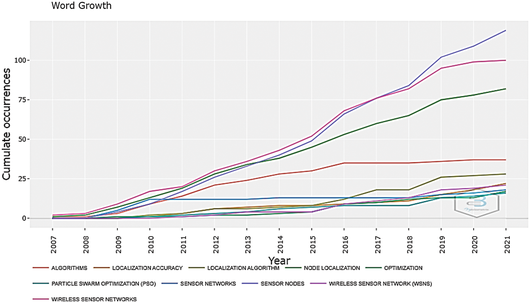
Figure 1: Yearly word growth in UWSN

The major contribution of this study is listed below:

•   Firstly, we have explained the basics of localization in UWSN, and statistical analysis is presented to motivate the researchers to explore the UWSN.

•   A three-layer classification of localization schemes established for UWSN is done to understand the detailed concepts in a stepwise manner.

•   A number of existing techniques for different localization schemes are reviewed and compared on the basis of certain parameters. Further, a performance analysis of these techniques is done. This will provide a status of progress and work which have been already done in this field to the researchers.

•   At the end, current research issues and future prospects regarding localization in UWSN are provided to give new directions to the researchers.

The remainder of the paper organization is given below. Classification of various localization schemes is done in Section 2. Also, various existing techniques are explained in this section. Next, Section 3 represents the comparative analysis of UWSN localization schemes based on various performance metrics. Section 4 discusses open research directions in UWSN. Finally, Section 5 brings the paper to a conclusion.

2  Classifications of Localization Schemes for UWSN

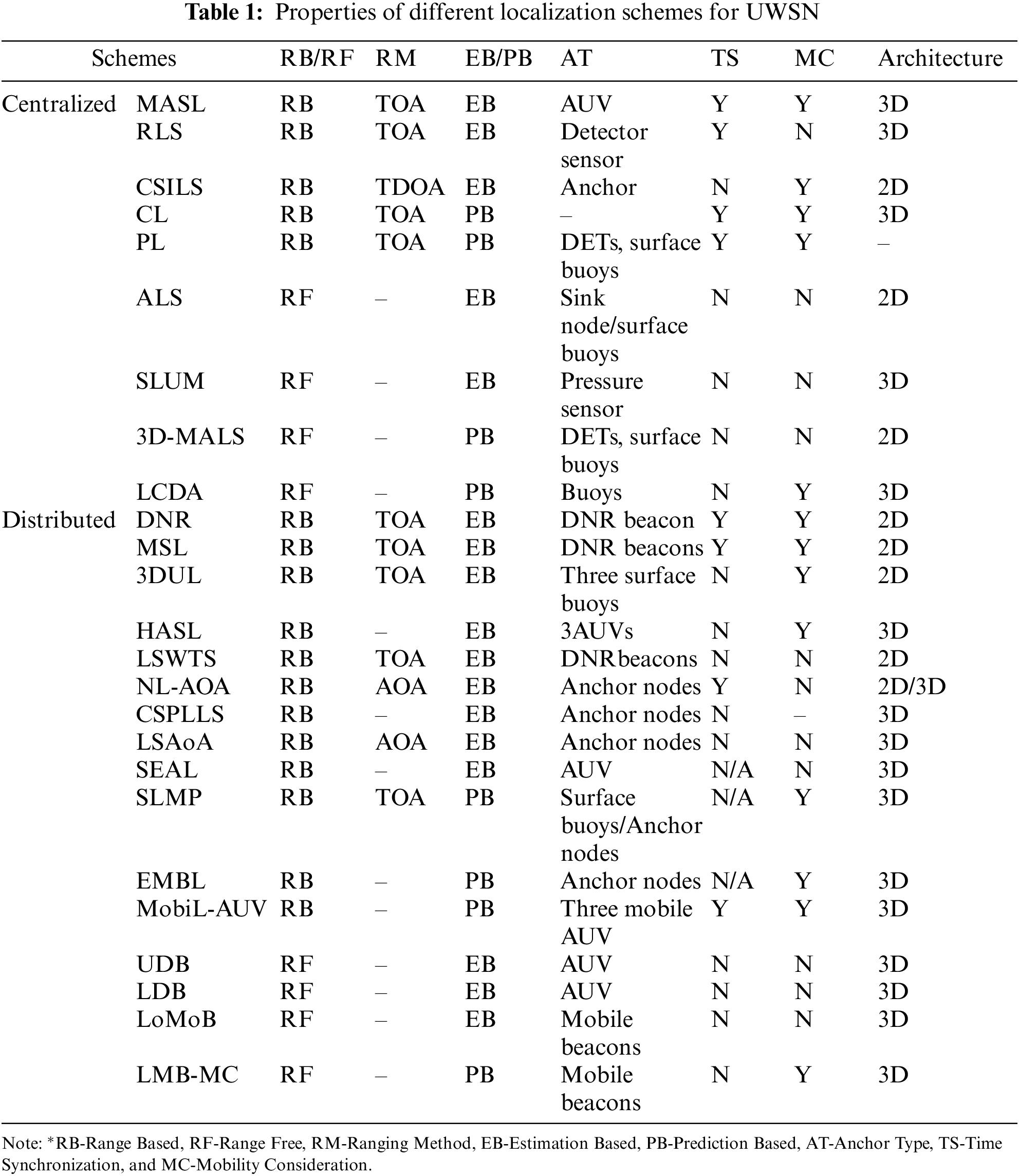
Here, localization schemes are divided into two categories as-centralized and distributed. These schemes are further classified into estimation-based and prediction-based localization strategies based on the ranging approach as per Fig. 2. The Properties of different localization schemes for UWSN is presented in Table 1.

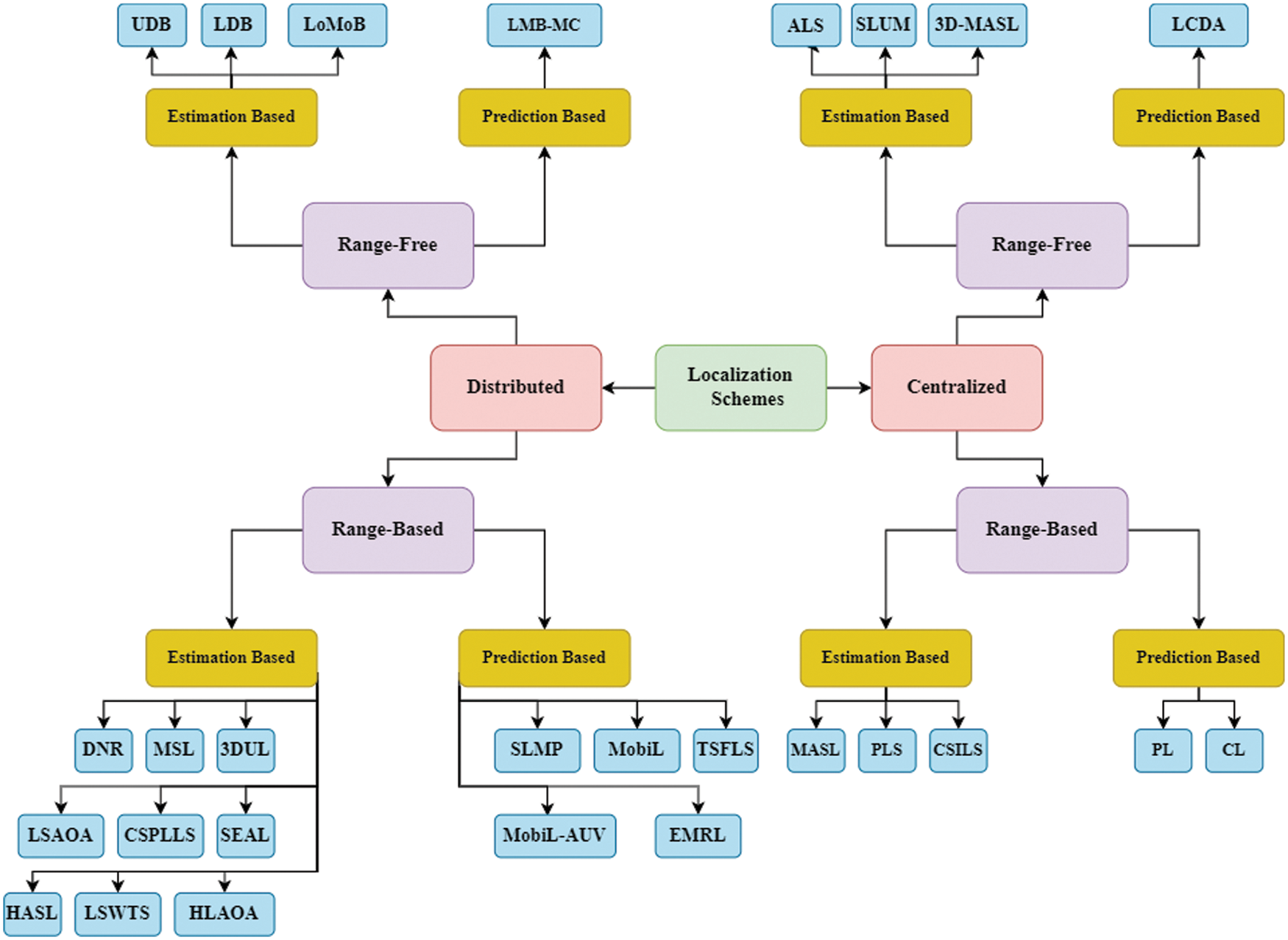
Figure 2: Classifications of localization schemes

•   Centralized vs. Distributed: In centralized localization, the location of each ordinary node in a command center is calculated. The ordinary node cannot find the location until the sink node explicitly communicates the data. At the end of the procedure, these approaches may be used to locate nodes. It indicates that it is at the post-processing stage; alternatively, they may collect information on a regular basis to monitor sensor nodes. Distributed localization approaches enable every ordinary node to conduct localization individually.

•   Range Based vs. Range-Free: Range-based algorithms utilize range or bearing data to find the position of ordinary nodes. For distance measurements, they need extra hardware, which will increase the price of the network. The propagation time is required for receiving the signal by the receiver [11,12]. This group of schemes provides a fine-grained estimation of the position. A number of ranging algorithmsTime of Arrival (TOA), Time Difference of Arrival (TDOA), Angle of Arrival (AOA) and Received Signal Strength Indicator (RSSI), based on distance, angle, and signal, respectively, are discussed in [13–16]. On the other hand, simple range-free localization techniques give coarse-grained position estimates because they do not require bearing data. There is no need for any additional hardware in these algorithms. These methods give a rough estimation of the sensor nodes position. A number of range-free algorithms are covered by researchers based on hop-count [17–19], area [20,21], and centroid [22–25], respectively.

•   Estimation Based vs. Prediction Based: The current position of the node is of relevance in estimation-based techniques, and it is derived using the most recent information available [26–30]. The position of the sensor node at the next time is estimated based on the distance that is past the locations of the node [30–33].

2.1 Centralized Localization Techniques

2.1.1 Range Based Schemes

A. Estimation Based Schemes

•   Motion Aware Self-Localization Scheme (MASL) [34,35]: Authors introduced a MASL scheme for mobile-based UWSN. The key aim of MASL is to discover the error in the process of distance estimation. At each iteration, the algorithm refines location distribution by dividing an event’s field into smaller grids and choosing the region in which nodes exist. The iterative method in this cannot offer real-time location data.

•   Reverse Localization Scheme (RLS) [36]: Here, researchers planned an event-based centralized localization algorithm called a Reverse localization scheme. The RLS method uses a reverse broadcasting phase. This reduced additional overhead, as well as the amount of messages, exchanged substantially. This method has two phases: transmission and localization. Detector sensors watch and detect an event in the first phase. Inthesecond phase, the sink node estimates the location of the detector sensor node as per Fig. 3.

Figure 3: Complete message format for RLS

This scheme [37] requires high energy due to time synchronization, whereas it provides low message exchange and achieves a high average response time. This scheme achieves 100% coverage by using the only 8% of anchor nodes. Whereas Seamless Message Protocol (SLMP) achieves 95% localization with 10% of anchor nodes [38].

•   Clock Synchronization Independent Localization Scheme (CSILS) [39]: CSILS scheme uses four anchor nodes with GPS receivers that find the location of sensor nodes. It contains three phases-(1) Determining distance variations using local clocks, (2) Calculating the distance variations into the location of the node, and (3) Deploying anchor nodes correctly. CSILS does not dependent on clock synchronization. This scheme improves localization accuracy. In the second phase, the sink node estimates the location of the detector sensor node as per Fig. 3.

B. Prediction-Based Schemes

•   Probabilistic Localization Scheme (PLS) [40,41]: To increase localization accuracy, a probabilistic localization technique is presented. Both uniform and normal error distributions are taken into account in this case. In this scheme, Normal distribution is used for measuring uncertainties as follows:

Mi=di+λ=di(1+p),where p∈[−∞,∞](1)

Here, di is the distance between the anchor and sensor nodes, and λ is the measurement error between these nodes (λ<<di). The Probabilistic Localization Method (PLM) technique [42] has two phases: At the first phase, every two neighboring anchor nodes use a circle-based technique to identify the locations of sensor nodes. The second step is to use the probability distribution to determine the final location of the sensor node. With additional anchor nodes, localization coverage and accuracy may be increased. However, computational complexity and energy consumption rise. The simulation findings show that the PLM approach may considerably enhance localization accuracy.

•   Collaborative Localization Scheme (CLS) [43]: CLS is a cost-effective and anchor–free self-localization technique. It does not need preceding node planning. In this scheme, sensor nodes are responsible for obtaining ocean depth data and then transferring it to the water surface. Here, profiler and follower are the two underwater sensor nodes. The profiler comes to go ahead with the follower. The distance between profiler and follower is periodically calculated by Time of Arrival (TOA) ranging method. Then the followers get the profiler’s location. CLS scheme is architectural dependent. To achieve high localization accuracy, the profiler should be closer to the follower; otherwise, localization failure will be occurred [44,45].

2.1.2 Range Free Schemes

A. Estimation Based Schemes

•   Area-Based Localization Scheme (ALS) [46]: An effective method of localization for a massive underwater sensor network is presented. This was created primarily for terrestrial WSNs [47]. This method was later modified for use by UWSN. The network is made up of different types of nodes: the reference node, sensor node, and sink node. Reference nodes transmit beacon signals to sensor nodes to help in their localization. By collecting the IDs of anchor nodes, sensor nodes monitor the signals based on their associated powers. The reported data is now sent to the sink node. ALS used the spherical model, which is represented in decibels as:

PLspr=20log⁡RRref(2)

where R is the distance from the sensor node to the target node, this is the distance in Eq. (2).

This process does not give the exact position of nodes. It reduces the total power utilization of underwater nodes and also enhances the network’s lifetime.

•   Silent Localization in Underwater using Magnetometers [48]: Authors introduced a centralized, range-free, and estimation-based localization scheme. Magnetometers and vessels with specified magnetic dipoles are utilized in this technique to silently locate the sensors. Here, the dipole creates the ferromagnetic field. This field is used for finding the location of underwater nodes [49]. This scheme has the following system model

xk+1=f(xk)+wk,yk=h(xk,uk,eku)+ek(3)

In this, f(x) is a nonlinear state transition function and wk is process noise. h(x) is a nonlinear measurement function and xk is the state vector, uk are inputs, eku is input noise and ek is measurement noise [50,51]. In this scheme, if a magnetometer is used, the localization accuracy is 26.1%, whereas ifGlobal Navigation Satellite System (GNSS) and magnetometer are used, then the accuracy is 12.9%.

•   3D Multi-Power Area Localization Scheme (MALS) [52]: A range-free 3D–MALS scheme is presented, which is based on mobile detachable elevator transceivers (DETs). The author also uses the idea of 2D-ALS in this scheme to reduce the localization error using the multi-power transmission. The spreading loss and attenuation loss of underwater acoustic waves are modeled as [53].

Ploss=20lg⁡RRref+1.0936(0.1f21+f2+40f24100+f2)(4)

Where Ploss be the total path loss, R be the distance between sources to destination, Rref is reference distance, and f is the frequency. Surface buoys, DETs, sink nodes, and sensor nodes are different types of nodes utilized in this structure. This technique improves the localization performance and reduces system costs.

B. Prediction-Based Schemes

Localization with Convolutional Denoising Autoencoder (LCDA) [54]: In this, the authors proposed a system based on a Convolutional Denoising Autoencoder (CDA). It takes a noisy bitmap as input representing the signal’s time-delay matrix and outputs matrix containing the target’s route purified from background and clutter noise. The suggested method is the first effort to use deep learning to detect targets in a reflected acoustic signal. The findings on both simulated and genuine signals demonstrated that this method is a potential alternative to more established approaches in terms of both performance and complexity.

2.2 Distributed Localization Techniques

2.2.1 Range-Based Schemes

A. Estimation Based Schemes

•   Dive and Rise Scheme (DNR) [55]: Authors suggested a localization technique named DNR localization. This is based on a mobile device or DNR beacons. The DNR beacons could stay at a certain depth. The total number of nodes in the network is denoted with N and N = DB + S, Where DB is the number of DNR beacons and S is the underwater unknown sensor nodes. The sensor nodes in DNR localization are assumed synchronized. Then it uses two schemes, Bounding Box and Triangulation, toevaluatethelocation of sensor nodes. This is a simple, silent, and energy-efficient scheme but it takes a longer time means it slows the speed of the localization process [56].

•   Multi-Stage Localization Scheme (MLS) [57]: MLS is implemented to address the coverage and delay concerns of Dive’n’Rise Localization (DNRL). Researchers did research on Multi-stage positioning by using Mobile beacons. This scheme uses an iterative procedure [58]. In order to approximate the location of the nodes via the iteration process, three sources are used. The sensor node coordinate (x, y, z) should satisfy the following:

di=(x−xi)2+(y−yi)2+(z−zi)2(5)

where di is the distance, i is the beacon id, and (xi, yi, zi) are the coordinates. The main advantage of MSL is high localization speed and reduction in deployment cost. However, it increases the expenses of high localization error and high communication overhead.

3-Dimensional Underwater Localization Scheme (3DUL) [59]: In this scheme, the author uses three surface buoys which relay their position coordinates to the neighboring nodes. Sensor nodes receive these three surface buoys locations. Then, by using ranging methods, these nodes calculate the distances to these surface buoys. In order to project an anchor node, each sensor node uses the following basic geometric equation:

r=d2−(zS−zA)2=c2t2−(zS−zA)2(6)

where r and d be the distances to the virtual anchor and the actual anchor. C represents sound speed; t represents propagation delay, zS represents sensor node depth, and zA Represents anchor node depth. Then it predicts its position by the trilateration method. The iterative process raises the localization errors due to the error occurrence in the distance calculation [60].

•   High-Speed Autonomous Underwater Vehicle (AUV)-Based Silent Localization Scheme (HASL) [61]: In this scheme, 3 AUVs are used. They travel down the center of the network to retain their trajectory using the dead reckoning method. In this, sensor node mobility is also considered.

Fig. 4 depicts the beacon message format. Every beacon message transmitted by the AUV includes the AUV ID as well as the AUV’s current position and time-stamp. The sensor nodes distinguish between two sets of beacon messages based on the time-stamp information [62,63]. All AUVs are time-synchronized & broadcast beacons together with the same speed to all sensor nodes. With a localization error of 2–7 meters, this scheme achieves above 90 percent localization coverage.

Figure 4: Message format for HASL

•   Localization Scheme without Time Synchronization (LSWTS) [64]: This scheme is an expansion of the DNR scheme, which eliminates the time synchronization criterion. In the DNR scheme, when beacon nodes receive their location, they vertically dive into the water and transmit localization messages at regular time intervals. When a node calculates its distance to three beacon nodes, then the trilateration method is used to find the position of sensor nodes. Although, nodes without time synchronization are located in LSWTS.

•   Node Localization with Angle of Arrival (AoA) assistance (NL-AOA) [65]: This scheme considers a static network. Sensor nodes calculate the AoA of the signal. It is obvious that a sensor node may connect with an anchor node through a much different number of hops. Assume a neighbor node Ni sends a message to a sensor node Nj. The sensor node Nj measures the AoA and extracts information from the communication message, adding the following to its information table as a new item. The entry’s specifics are as follows as per Fig. 5.

Figure 5: Sensor node’s information table

This scheme has two steps: distance calculation & location estimation. At the first step, distance is calculated using AOA & in the second step, the weighted least square (WLS) method is utilized to calculate the position of ordinary nodes. The distances are measured by a sensor node at four anchors to estimate its position; nodes apply the weighted least square rule [66].

•   Localization Scheme using AoA Technique (LSAOA) [67]: This scheme has three phases: the angle is estimated first, then the projection phase, and the final phase is the localization of the node. In the first phase, sensor nodes measure the angle of the arrival for each signal. Then inthesecond phase, a 3D localization problem is converted into the 2D by projection process and calculated:

d1=d2−(za−zb)2(7)

d2=AR2+(Zf−Za)2−2(AR)(|Zf−Za|)Cosθ1(8)

This scheme has enormous achievements in localization and high coverage in the underwater network [68].

•   Communication Signal Propagation Loss Localization Scheme (CSPLLS) [69]: This is an asynchronous, cooperative, passive, and distributed method. Here, the sensor node uses signal strength from reference nodes. This method is highly applicable for monitoring the underwater environment and navigation of the target in the ocean.

•   Self-adaptive AUV-based Localization Scheme (SEAL) [70,71]: Authors presented a localization scheme that uses Self-adaptive AUV instead of a surface-based anchor. These AUVs intelligently adjust the transmission range. The inter-node and node-AUV distance can be determined by AUVs. In this scheme, the coverage area of localization rises up to 80% compare to DNRL. Approximately 52%, 16%, 35%, and 16% high compared to the Three Dimensional Localization Algorithm (3-DUL), MSL, and HASL schemes, correspondingly. As well as, this scheme maintains low power utilization of the sensor node.

B. Prediction Based Schemes

•   Scalable Localization with Mobility Prediction Scheme (SLMP) [72]: SLMP is a distributed and prediction-based scheme. In this, localization is calculated in a hierarchical way same as LSL. Among other less effective underwater sensors, the anchors are positioned under the water but can self-localize through direct contact with four surface buoys. Anchor nodes would control the whole process of localization.

N-ID is the message sender’s unique identifying number. The T-stamp indicates the time when the message was sent. The sender’s current location is indicated in the Location field. The anticipated speed vector for the next window is called the S-vector. C-Value is the message sender’s level of confidence as per Fig. 6. It is used to indicate the precision of position estimates [73].

Figure 6: Packet format for SLMP

•   Mobility-Assisted Localization Scheme (MALS) [74]: In this scheme, three anchor nodes are used on the surface. The localization process in this scheme is divided into two stages which are Mobility prediction and Ranging and Localization. At the first level, by analyzing the mobility pattern of nearest neighbors, each sensor node forecasts its mobility pattern. At the second level, sensor nodes are positioned automatically by listening to the beacon packet from the anchor nodes. Here, the position prediction will be faster and have less power consumption leading to the passive receiving of beacon signals.

•   MobiL-AUV Aided Scheme [75]: In this scheme, three moving AUVs are deployed to a specific depth underwater. This scheme consists of two phases which are mobility prediction and localization process. In the first phase, sensor nodes estimate their mobility by using the moving pattern of the nearest nodes. At the localization phase, ordinary nodes receive beacon messages from MobiL-AUVs. After that, these nodes get localized by using different Computational methods. The MobiL-AUV covers a wide area, thus becoming a reference node for other sensor nodes [76]. A minimal localization error is accomplished by providing a minimum gap between AUVs and ordinary nodes.

•   Time–Synchronization Free Localization Scheme (TSFLS) with Mobility Prediction for UWSN [77]: This scheme includes the moving behavior of sensor nodes on the localization as per Fig. 7. The moving sensor nodes in the water result in inaccuracy in the location calculation. This uses mobile beacons, which move toward the floor of the ocean. Each mobile beacon has a message which contains different fields.

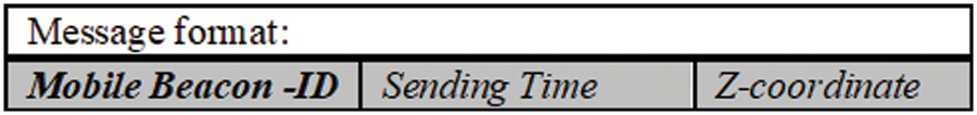
Figure 7: Message format for TSFLS

Then the mobile beacons move back to the surface and update their position via GPS and transmit this to neighbor nodes. This scheme increases the localization accuracy by predicting the mobility behavior of sensor nodes.

•   Efficient Mobility-Based Localization (EMBL) [78]: Authors projected a prediction-based scheme for the underwater environment. This scheme also determines the position of ordinary nodes underwater based on the mobility prediction model. This scheme has two phases: anchor node localization and sensor node localization. In this process, the future position of the ordinary nodes is calculated with the past location of sensor nodes. This scheme reduces the localization cost of the network.

2.2.2 Range-Free Schemes

A. Estimation Based Schemes

•   Utilizes Directional Beacons (UDB) Scheme [79–82]: Scientists presented a localization scheme by using directional beacons. A pre-defined path is covered by an AUV having a directional antenna. Ordinary nodes silently receive these signals. After that, they confine their coordinates. This is a less power-consuming method. Time synchronization among nodes is not required in this.

•   Localization with Directional Beacons (LDB): This scheme can be applied for both dense and sparse 3D UWSN. LDB scheme is the extended form of the UDB scheme in the 3D underwater network. An AUV with a directional antenna moves over the 3D network by deploying nodes at different depths. In this, the nodes listen to the beacon message, which falls in the conical beacon beam. With the constant depth, the center of the circle is as follows:

r=tan⁡(α2)×Δh (9)

where h is the depth of the node and α is the angle of the conical beacon, and Δh = |hA−h|. As a result, we could map the nodes from 3D to 2D with specified circles when the AUV travels at a given depth of water, transmitting beacons. This method consumes less power as they use silent localization. In this scheme, AUVs need to navigate the network more than one time to cover the entire network, as it is only capable of sending beacons in one direction [83–86].

•   Localization with Mobile Beacon (LoMoB): This scheme considers a system that uses an omnidirectional antenna. This is an extension of the framework of the LDB that employs a directional antenna. In this, the mobile beacons pass across the surface of the water. Here, due to the use of the omnidirectional antenna, the 3D motion of the mobile beacons is possible. It uses the selection and projection process for beacon points same as the LDB scheme. The sensor nodes receive this message within the mobile beacon’s communication range. Then using the weighted average of the potential positions, the location of the sensor node is calculated. The distance between the projected beacon node and the sensor node is as follows:

(r−d/2)2−(zi−zs)2(10)

where a sensor node’s z coordinates and the ith beacon point’s z coordinates are zs and zi. As compared to LDB, this method improves the average localization error and localization accuracy [87–90].

B. Prediction-Based Schemes:

•   Localization via Motion Compensation (LMB-MC): This scheme also uses the directional antenna for communication. This system can reduce beacon point uncertainty by compensating for the passive motion of the AUVs or ships. Whereas by using ellipse-based models, geometric shape instability can be minimized. This scheme reduces the localization error as compared to LDB and LoMoBschemes [91–93].

3  Conclusion

For the evaluation purpose of localization schemes, as discussed in localization coverage, localization error, localization time, and communication cost are considered performance metrics. The results in Fig. 8 show that MobiL–AUV and TSFLS localization schemes outperform in comparison rest all localization schemes in terms of localization coverage. Fig. 9 represents the MobiL-AUV scheme and LDB scheme with maximum and minimum average localization error, respectively. Fig. 10 shows the SEAL scheme with a maximum average localization delay. Fig. 11 represents the 3DUL scheme with the highest communication cost [94].

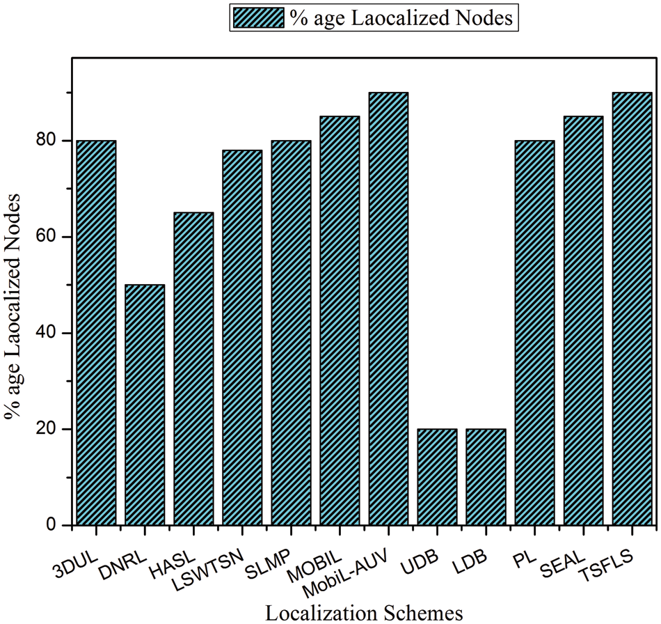
Figure 8: Comparison of localization coverage

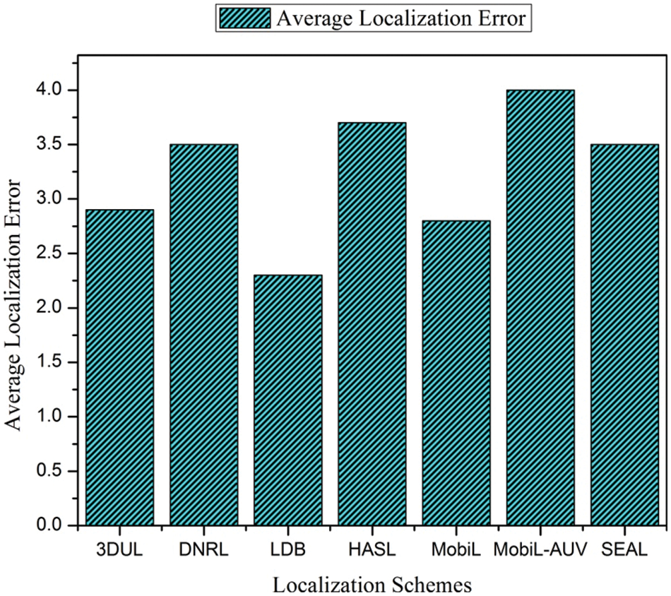
Figure 9: Comparison of localization error

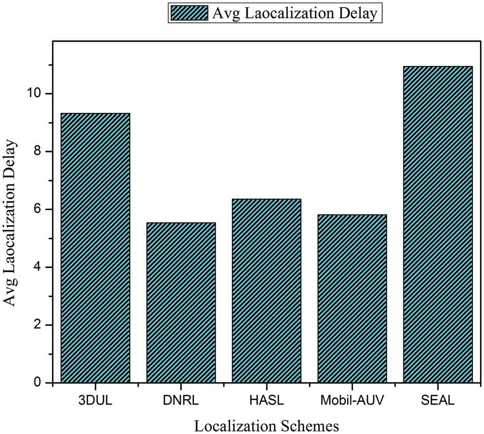
Figure 10: Comparison of localization delay

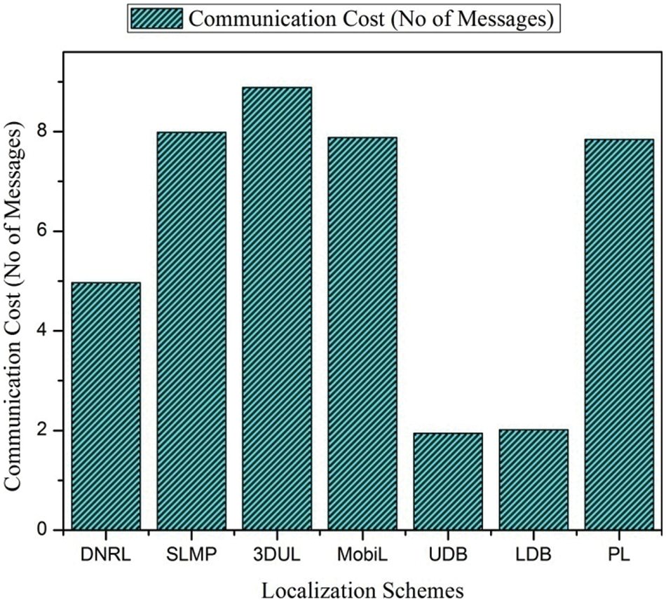
Figure 11: Comparison of communication cost

4  Open Research Directions

The various challenges associated with the UWSN are severely limited bandwidth, moving sensor nodes, and limited battery power because these cannot be charged due to a lack of solar energy underwater. A discussion on these challenges is presented below:

•   Node movement induced by water current is one of the most serious challenges for underwater localization. Therefore, a more realistic mobility model that incorporates sensor node movement in diverse operational situations and settings is required.

•   Constant sound speed is considered for most of the proposed localization approaches underwater. However, the sound speed in water changes with depth, temperature, and salinity. As a result, assuming constant sound speed may affect accuracy in estimating sensor node locations.

•   Several schemes have been developed for securing the localization process in terrestrial WSNs. In most UWSN localization techniques, security issues are neglected. An attack on the localization infrastructure might endanger the entire sensing operation by connecting sensed data to inaccurate locations.

•   UWSN is considered a foundation for creating a new 5G wireless networking environment in the future. The ability to acquire large data rates and monitor underwater activities more accurately is dependent on the 5G network.

With the growth of wireless technologies, UWSN has fascinated a large number of scientists and has made important contributions in this sector. However, the door is still open for future study and prospects.

Acknowledgement: The authors would like to thank the editors of CMC and anonymous reviewers for their time and reviewing this manuscript.

Funding Statement: The authors received specific funding for this study.

Conflicts of Interest: The authors declare that they have no conflicts of interest to report regarding the present study.

References

1. S. N. Atluri and S. Shen, “Global weak forms, weighted residuals, finite elements, boundary elements & local weak forms,” in The Meshless Local Petrov-Galerkin (MLPG) Method, 1st ed., vol. 1. Henderson, NV, USA: Tech Science Press, pp. 15–64, 2004. [Google Scholar]

2. F. Emad, F. K. Shaikh, U. M. Qureshi, A. A. Sheikh and S. B. Qaisar, “Underwater sensor network applications: A comprehensive survey,” International Journal of Distributed Sensor Networks, vol. 11, no. 11, pp. 896832–896856, 2015. [Google Scholar]

3. J. Mohammed, K. Ibrahimi, H. Tembine and J. B. Othman, “Underwater wireless sensor networks: A survey on enabling technologies, localization protocols, and internet of underwater things,” IEEE Access, vol. 7, no. 5, pp. 96879–96899, 2019. [Google Scholar]

4. P. Jim, J. Kurose and B. N. Levine, “A survey of practical issues in underwater networks,” ACM SIGMOBILE Mobile Computing and Communications Review, vol. 11, no. 4, pp. 23–33, 2007. [Google Scholar]

5. H. John, W. Ye, J. Wills, A. Syed and Y. Li, “Research challenges and applications for underwater sensor networking,” in IEEE Wireless Communications and Networking Conf., WCNC 2006, Las Vegas, NV, vol. 1, pp. 228–235, 2006. [Google Scholar]

6. C. J. Hong, J. Kong, M. Gerla and S. Zhou, “The challenges of building mobile underwater wireless networks for aquatic application,” IEEE Network, vol. 20, no. 3, pp. 12–18, 2006. [Google Scholar]

7. T. Gurkan and V. C. Gungor, “A survey on deployment techniques, localization algorithms, and research challenges for underwater acoustic sensor networks,” International Journal of Communication Systems, vol. 30, no. 17, pp. 3350–3376, 2017. [Google Scholar]

8. S. Xin, I. Ullah, X. Liu and D. Choi, “A review of underwater localization techniques, algorithms, and challenges,” Journal of Sensors, vol. 7, no. 6, pp. 567–579, 2020. [Google Scholar]

9. A. Rajagopal, S. Somasundaram, B. Sowmya and T. Suguna, “Soft computing based cluster head selection in wireless sensor network using bacterial foraging optimization algorithm,” International Journal of Electronics and Communication Engineering, vol. 3, no. 3, pp. 379–384, 2015. [Google Scholar]

10. M. Beniwal and R. Singh, “Localization techniques and their challenges in underwater wireless sensor networks,” International Journal of Computer Science and Information Technologies, vol. 3, no. 5, pp. 4706–4710, 2014. [Google Scholar]

11. H. P. Tan, R. Diamant, W. K. Seah and M. Waldmeyer, “A survey of techniques and challenges,” IEEE Access, vol. 4, no. 5, pp. 5678–5686, 2014. [Google Scholar]

12. J. Mullica, K. Jaroensutasinee, S. J. Bainbridge, T. Fountain, S. Chumkiew et al., “Sensor networks applications for reefs at Racha Island, Thailand,” in Proc. of the 12th Int. Coral Reef Symp., Cairns, Australia, pp. 95–115. 2012. [Google Scholar]

13. J. Bachrach and C. Taylor, “Localization in sensor networks,” Handbook of Sensor Networks, vol. 12, no. 1, pp. 277–310, 2005. [Google Scholar]

14. F. Zhao, J. G. Leonidas and G. Leonidas, “An information processing approachinWireless sensor networks,” Morgan Kaufmann, vol. 3, no. 1, pp. 45–57, 2004. [Google Scholar]

15. I. Ullah, Y. Liu, X. Su and P. Kim, “Efficient and accurate target localization in underwater environment,” IEEE Access, vol. 7, no. 2, pp. 101415–101426, 2019. [Google Scholar]

16. E. K. Melike, H. T. Mouftah and S. Oktug, “A survey of architectures and localization techniques for underwater acoustic sensor networks,” IEEE Communications Surveys & Tutorials, vol. 13, no. 3, pp. 487–502, 2011. [Google Scholar]

17. S. Yanlong, Y. Yuan, X. Qimin, H. Changchun and X. Guan, “A mobile anchor node assisted RSSI localization scheme in underwater wireless sensor networks,” Sensors, vol. 20, no. 3, pp. 4369–4383, 2019. [Google Scholar]

18. N. Dragoş and B. Nath, “DV based positioning in ad hoc networks,” Telecommunication Systems, vol. 22, no. 1, pp. 267–280, 2003. [Google Scholar]

19. C. Rabaey, J. Savarese and K. Langendoen, “Robust positioning algorithms for distributed ad-hoc wireless sensor network,” in USENIX Technical Annual Conf., Monterrey, CA, pp. 317–327, 2002. [Google Scholar]

20. W. S. Yee, J. G. Lim, S. V. Rao and W. Seah, “Multihop localization with density and path length awareness in non-uniform wireless sensor networks,” in 2005 IEEE 61st Vehicular Technology Conf., Stockholm, Sweden, vol. 4, pp. 2551–2555, 2005. [Google Scholar]

21. C. Vijay and W. Seah, “An area localization scheme for underwater sensor networks,” in OCEANS 2006-Asia Pacific, Singapore, pp. 1–8, 2006. [Google Scholar]

22. H. Tian, C. Huang, B. M. Blum, J. A. Stankovic and T. Abdelzaher, “Range-free localization schemes for large scale sensor networks,” in Proc. of the 9th Annual Int. Conf. on Mobile Computing and Networking, New York, NY, United States, pp. 81–95, 2003. [Google Scholar]

23. C. Hongyang, P. Huang, M. Martins, H. C. So and K. Sezaki, “Novel centroid localization algorithm for three-dimensional wireless sensor networks,” in 4th Int. Conf. on Wireless Communications, Networking and Mobile Computing, Dalian, China, pp. 1–4, 2008. [Google Scholar]

24. E. K. Melike, S. Oktug, L. Vieira and M. Gerla, “Performance evaluation of distributed localization techniques for mobile underwater acoustic sensor networks,” Ad Hoc Networks, vol. 9, no. 1, pp. 61–72, 2011. [Google Scholar]

25. Q. U. Fengzhong, W. Shiyuan, W. U. Zhihui and L. I. U. Zubin, “A survey of ranging algorithms and localization schemes in underwater acoustic sensor network,” China Communications, vol. 13, no. 3, pp. 66–81, 2016. [Google Scholar]

26. A. S. Faiza, N. Alzeidi and K. Day, “Localization schemes for underwater wireless sensor networks: Survey,” International Journal of Computer Networks & Communications (IJCNC), vol. 12, no. 2, pp. 113–130, 2020. [Google Scholar]

27. X. Tao, Y. Hu, B. Zhang and G. Leus, “RSS-based sensor localization in underwater acoustic sensor networks,” in IEEE Int. Conf. on Acoustics, Speech and Signal Processing (ICASSP), Shanghai, China, pp. 3906–3910, 2016. [Google Scholar]

28. M. Gupta and A. K. Nagawat, “Design and implementation of high performance advanced extensible interface (AXI) based DDR3 memory controller,” in 2016 Int. Conf. Communication and Signal Processing (ICCSP), Melmaruvathur, India, pp. 1175–1179, 2016. [Google Scholar]

29. A. Mesmoudi, F. Mohammed and L. Nabila, “Wireless sensor networks localization algorithms: A comprehensive survey,”International Journal of Computer Networks & Communications (IJCNCArxiv Preprint Arxiv, vol. 1312, pp. 4082–4099, 2013. [Google Scholar]

30. N. Ibrahim, T. Sheltami, E. Shakshuki, A. AElkhail and A. Mumin, “Performance evaluation of range-free localization algorithms for wireless sensor networks,” Personal and Ubiquitous Computing, vol. 25, no. 1, pp. 177–203, 2021. [Google Scholar]

31. K. Mal, I. H. Kalwar, K. Shaikh, T. D. Memon, B. S. Chowdhry et al., “A new estimation of nonlinear contact forces of railway vehicle,” Intelligent Automation and Soft Computing, vol. 28, no. 3, pp. 823–841, 2021. [Google Scholar]

32. E. M. Kantarci, H. T. Mouftah and S. Oktug, “Localization techniques for underwater acoustic sensor networks,” IEEE Communications Magazine, vol. 48, no. 12, pp. 152–158, 2010. [Google Scholar]

33. D. Mirza and C. Schurgers, “Motion-aware self-localization for underwater networks,” in Proc. of the Third ACM Int. Workshop on Underwater Networks, San Francisco, California, USA, pp. 51–58, 2008. [Google Scholar]

34. M. Marjan, J. Rezazadeh and A. S. Ismail, “A reverse localization scheme for underwater acoustic sensor networks,” Sensors, vol. 12, no. 4, pp. 4352–438, 2012. [Google Scholar]

35. C. Bechaz and H. Thomas, “GIB system: The underwater GPS solution,” in Proc. of the Fifth Europe Conf. on Underwater Acoustics (ECUA, 2000), ESCPE Lyon, France, pp. 843–848, 2000. [Google Scholar]

36. D. Yuhan, R. Wang, Z. Li, C. Cheng and K. Zhang, “Improved reverse localization schemes for underwater wireless sensor networks,” in Proc. of the 16th ACM/IEEE Int. Conf. on Information Processing in Sensor Networks, Pittsburgh (Pennsylvaniapp. 323–324, 2017. [Google Scholar]

37. Z. Qiang, Z. Senlin and L. Meiqin, “A clock synchronization independent localization scheme for underwater wireless sensor networks,” in Proc. of the Eighth ACM Int. Conf. on Underwater Networks and Systems, Kaohsiung Taiwa, pp. 1–5, 2013. [Google Scholar]

38. B. Tao, R. Venkatesan and C. Li, “Design and evaluation of a new localization scheme for underwater acoustic sensor network,” in GLOBECOM IEEE Global Telecommunications Conf., Honolulu, HI, USA, pp. 1–5, 2009. [Google Scholar]

39. K. C. Lee, Q. J. Sian and M. C. Huang, “Underwater acoustic localization by principal components analyses based probabilistic approach,” Applied Acoustics, vol. 70, no. 9, pp. 1168–1174, 2009. [Google Scholar]

40. L. Xinrong, “Collaborative localization with received-signal strength in wireless sensor networks,” IEEE Transactions on Vehicular Technology, vol. 56, no. 6, pp. 3807–3817, 2007. [Google Scholar]

41. Z. Chenyu, G. Han, J. Jiang, L. Shu, G. Liu et al., “A collaborative localization algorithm for underwater acoustic sensor networks,” in Int. Conf. on Computing, Management and Telecommunications (Com ManTel), Da Nang, Vietnam, pp. 211–216, 2014. [Google Scholar]

42. G. Han, J. Jiang, L. Shu, Y. Xu, F. Wang, “Localization algorithms of underwater wireless sensor networks: A survey,” Sensors (Basel), vol. 12, no. 2, pp. 2026–61. 2012. https://doi.org/10.3390/s120202026. Epub 2012 Feb 13. PMID: 22438752; PMCID: PMC3304154. [Google Scholar] [PubMed] [CrossRef]

43. M. Gupta, H. Taneja, L. Chand and V. Goyal, “Enhancement and analysis in MRI image denoising for different filtering techniques,” Journal of Statistics and Management System, vol. 21, no. 4, pp. 561–568, 2018. [Google Scholar]

44. Y. Qi, S. K. Tan, Y. Ge, B. S. Yeo and Q. Yin, “An area localization scheme for large wireless sensor networks,” in 2005 IEEE 61st Vehicular Technology Conf., Stockholm, Sweden, vol. 5, pp. 2835–2839, 2005. [Google Scholar]

45. C. Jonas, M. Skoglund and F. Gustafsson, “Silent localization of underwater sensors using magnetometers,” Eurasip Journal on Advances in Signal Processing, vol. 56, no. 2, pp. 1–8, 2010. [Google Scholar]

46. Y. Zhou, C. Xiao and G. Zhou, “Multi-objectivization-based localization of underwater sensors using magnetometers,” IEEE Sensors Journal, vol. 14, no. 4, pp. 1099–1106, 2013. [Google Scholar]

47. T. I. Fossen and T. Perez, “Marine systems simulator (MSS). 2004,” URL https://github.com/cybergalactic/MSS, 2004. [Google Scholar]

48. F. Gustafsson, Adaptive Filtering and Change Detection, vol. 2. Hoboken, NJ, USA: John Wiley & Sons, 2001. [Google Scholar]

49. S. Xin, I. Ullah, X. Liu and D. Choi, “A review of underwater localization techniques, algorithms, and challenge,” Journal of Sensors, vol. 78, no. 3, pp. 346–359, 2020. [Google Scholar]

50. T. H. William, “Analytic description of the low-frequency attenuation coefficient,” The Journal of the Acoustical Society of America, vol. 42, no. 1, pp. 270–270, 1967. [Google Scholar]

51. R. J. Urick, “Low-frequency sound attenuation in the deep ocean,” The Journal of the Acoustical Society of America, vol. 35, pp. 1413–1422, 1963. [Google Scholar]

52. E. Melike, L. F. M. Vieira and M. Gerla, “Localization with dive’N’Rise (DNR) beacons for underwater acoustic sensor networks,” in Proc. of the Second Workshop on Underwater Networks, Montréal, Québec, Canada, pp. 97–100, 2007. [Google Scholar]

53. C. Kai, Y. Zhou and J. He, “A localization scheme for underwater wireless sensor networks,” International Journal of Advanced Science and Technology, vol. 4, no. 2, pp. 342–355, 2009. [Google Scholar]

54. E. Melike, L. F. M. Vieira, A. Caruso, F. Paparella, M. Gerla et al., “Multi stage underwater sensor localization using mobile beacons,” in Second Int. Conf. on Sensor Technologies and Applications (Sensorcomm 2008), Cap Esterel, France, pp. 710–714, 2008. [Google Scholar]

55. I. Tariq and Y. K. Lee, “A two-stage localization scheme with partition handling for data tagging in underwater acoustic sensor networks,” Sensors, vol. 19, no. 9, pp. 2135, 2019. [Google Scholar]

56. M. I. Talha and O. B. Akan, “A three-dimensional localization algorithm for underwater acoustic sensor networks,” IEEE Transactions on Wireless Communications, vol. 8, no. 9, pp. 4457–4463, 2009. [Google Scholar]

57. Z. Zhong, J. H. Cui and S. Zhou, “Localization for large-scale underwater sensor networks, “ in Int. Conf. on Research in Networking, Berlin, Heidelberg, Springer, pp. 108–119, 2007. [Google Scholar]

58. T. Ojha and S. Misra, “HASL: High-speed AUV-based silent localization for underwater sensor networks,” in Int. Conf. on Heterogeneous Networking for Quality, Reliability, Security and Robustness, Greader Noida, India, pp. 128–140, 2013. [Google Scholar]

59. E. Melike, L. M. F. Vieira and M. Gerla, “AUV-aided localization for underwater sensor networks,” in Int. Conf. on Wireless Algorithms, Systems and Applications, Chicago, IL, USA, IEEE, pp. 44–54, 2007. [Google Scholar]

60. W. Marc, H. P. Tan and W. K. G. Seah, “Multi-stage AUV-aided localization for underwater wireless sensor networks,” in 2011 IEEE Workshops of Int. Conf. on Advanced Information Networking and Applications, Biopolis, Singapore, pp. 908–913, 2011. [Google Scholar]

61. M. Beniwal, R. Singh and A. Sangwan, “A localization scheme for underwater sensor networks without time synchronization,” Wireless Personal Communications, vol. 88, no. 3, pp. 537–552, 2016. [Google Scholar]

62. H. Huai and Y. R. Zheng, “Node localization with AoA assistance in multi-hop underwater sensor networks,” AdhocNetworks, vol. 78, no. 1, pp. 32–41, 2018. [Google Scholar]

63. S. Olga, “Least-squares rigid motion using svd, ” Technical Notes, vol. 120, no. 3, pp. 52–68, 2009. [Google Scholar]

64. M. Gupta, J. Lechner and B. Agarwal, “Performance analysis of Kalman filter in computed tomography thorax for image denoising,” Recent Advances in Computer Science and Communications, vol. 13, no. 6, pp. 1199–1212, 2020. [Google Scholar]

65. T. Archana, R. Singh and S. Das, “A localization scheme for underwater acoustic wireless sensor networks using AoA,” Recent Advances in Computer Science and Communications, vol. 14, no. 3, pp. 690–699, 2021. [Google Scholar]

66. Q. Gang, C. Zhao, F. Zhou and N. Ahmed, “Distributed localization based on signal propagation loss for underwater sensor networks,” IEEE Access, vol. 7, no. 3, pp. 112985–112995, 2019. [Google Scholar]

67. T. Ojha, S. Misra and S. M. Obaidat, “SEAL: Self-adaptive AUV-based localization for sparsely deployed underwater sensor networks,” Computer Communications, vol. 154, no. 3, pp. 204–215, 2020. [Google Scholar]

68. B. Pierpaolo and G. Mazzini, “Localization in sensor networks with fading and mobility,” in The 13th IEEE Int. Symp. on Personal, Indoor and Mobile Radio Communications, Lisbon, Portuga, vol. 2, pp. 750–754, 2002. [Google Scholar]

69. G. Silke, R obust Adaptation to non-Native Accents in Automatic Speech Recognition. Berlin, Heidelberg: Springer, pp. 897–912, 2002. [Google Scholar]

70. T. Ojha and S. Misra, “Mobil: A 3-dimensional localization scheme for mobile underwater sensor networks,” in 2013 National Conf. on Communications (NCC), New Delhi, India, pp. 1–5, 2013. [Google Scholar]

71. M. Hammad, N. Javaid, A. Yahya, B. Ali, Z. A. Khan et al., “Mobil-AUV: AUV-aided localization scheme for underwater wireless sensor networks,” in 10th Int. Conf. on Innovative Mobile and Internet Services in Ubiquitous Computing (IMIS), Fukuoka, Japan, pp. 170–175, 2016. [Google Scholar]

72. J. Nadeem, H. Maqsood, A. Wadood, I. A. Niaz, A. Almogren et al., “A localization based cooperative routing protocol for underwater wireless sensor networks,” Mobile Information Systems, vol. 45, no. 2, pp. 568–579, 2017. [Google Scholar]

73. T. Archana, R. Singh and S. Das, “Time-synchronization free localization scheme with mobility prediction for UAWSNs,” Recent Advances in Computer Science and Communications (Formerly: Recent Patents on Computer Science), vol. 14, no. 3, pp. 700–709, 2021. [Google Scholar]

74. P. T. V. Bhuvaneswari, S. Karthikeyan, B. Jeeva and M. A. Prasath, “An efficient mobility based localization in underwater sensor networks,” in 2012 Fourth Int. Conf. on Computational Intelligence and Communication Networks, Mathura, India, pp. 90–94, 2012. [Google Scholar]

75. L. Hanjiang, Y. Zhao, Z. Guo, S. Liu, P. Chen et al., “UDB: Using directional beacons for localization in underwater sensor networks.” in 2008 14th IEEE Int. Conf. on Parallel and Distributed Systems, Melbourne, VIC, Australia, pp. 551–558, 2008. [Google Scholar]

76. L. Hanjiang, Z. Guo, W. Dong, F. Hong and Y. Zha, “LDB: Localization with directional beacons for sparse 3D underwater acoustic sensor networks,” Journal of Networks, vol. 5, no. 1, pp. 28–56, 2010. [Google Scholar]

77. L. Sangho and K. Kim, “Localization with a mobile beacon in underwater acoustic sensor networks,” Sensors, vol. 12, no. 5, pp. 5486–5501, 2012. [Google Scholar]

78. K. Yonghun, M. E. Kantarci, Y. Noh and K. Kim, “Range-free localization with a mobile beacon via motion compensation in underwater sensor networks,” IEEE Wireless Communications Letters, vol. 10, no. 1, pp. 6–10, 2020. [Google Scholar]

79. K. Nisar, M. H. A. Hijazi and I. A. Lawal, “A new model of application response time for VoIP over WLAN and fixed WiMAX,” in 2015 IEEE Second Int. Conf. on Computing Technology and Information Management (ICCTIM), Johor, Malaysia, pp. 174–179, 2015. [Google Scholar]

80. S. K. Memon, K. Nisar and W. Ahmad, “Performance evaluation of densely deployed WLANs using directional and omni-directional antennas,” in Computational Science and Technology, 1st ed., Kota Kinabalu, Malaysia, Springer, pp. 369–378, 2019. [Google Scholar]

81. M. R. Haque, S. C. Tan, Z. Yusoff, K. Nisar, C. K. Lee et al., “SDN architecture for UAVs and EVs using satellite: A hypothetical model and new challenges for future,” in IEEE 18th Annual Consumer Communications & Networking Conf. (CCNC), Las Vegas, NV, USA, pp. 1–6, 2021. [Google Scholar]

82. E. R. Jimson, K. Nisar and M. H. A. Hijazi, “The state of the art of software defined networking (SDN) issues in current network architecture and a solution for network management using the SDN,” International Journal of Technology Diffusion (IJTD), vol. 10, no. 3, pp. 33–48, 2019. [Google Scholar]

83. N. Salam, M. K. Abbas, M. K. Maheshwari, B. S. Chowdhry and K. Nisar, “Future mobile technology: Channel access mechanism for LTE-LAA using deep learning,” in IEEE 18th Annual Consumer Communications & Networking Conf. (CCNC), Las Vegas, NV, USA, pp. 1–5, 2021. [Google Scholar]

84. M. R. Haque, S. C. Tan, Z. Yusoff, K. Nisar, C. K. Lee et al., “A novel DDoS attack-aware smart backup controller placement in SDN design,” Annals of Emerging Technologies in Computing (AETiC), vol. 34, no. 1, pp. 2516–25, 32, 2020. [Google Scholar]

85. K. Nisar, A. M. Said and H. Hasbullah, “A voice priority queue (VPQ) fair scheduler for the VoIP over WLANs,” International Journal on Computer Science and Engineering (IJCSE), vol. 3, no. 2, pp. 506–518, 2011. [Google Scholar]

86. K. Mal, I. H. Kalwar, K. Shaikh, T. D. Memon, B. S. Chowdhry et al., “A new estimation of nonlinear contact forces of railway vehicle,” Intelligent Automation & Soft Computing, vol. 28, no. 3, pp. 546–563, 2021. [Google Scholar]

87. M. R. Haque, S. C. Tan, Z. Yusoff, K. Nisar, R. Kaspin et al., “Unprecedented smart algorithm for uninterrupted SDN services during DDoS attack,” Computers, Materials & Continua, vol. 70, no. 1, pp. 875–894, 2022. [Google Scholar]

88. M. R. Haque, S. C. Tan, Z. Yusoff, K. Nisar, C. K. Lee et al., “Automated controller placement for software-defined networks to resist DDoS attacks,” Computers, Materials & Continua, vol. 68, no. 3, pp. 3147–3165, 2021. [Google Scholar]

89. A. Adarsh, B. Kumar, M. Gupta, A. Kumar, A. Singh et al., “Design of an efficient cooperative spectrum for intra-hospital cognitive radio network,” Computers, Materials & Continua, vol. 69, no. 1, pp. 35–49, 2021. [Google Scholar]

90. M. M. Saeed, M. K. Hasan, R. Hassan, R. Mokhtar, R. A. Saeed et al., “Preserving privacy of user identity based on pseudonym variable in 5G,” Computers, Materials & Continua, vol. 70, no. 3, pp. 5551–5568, 2022. [Google Scholar]

91. L. Vyas and M. Gupta, “Routing in wireless sensor networks with asymmetric links,” Annals of the Romanian Society for Cell Biology, vol. 6, no. 3, pp. 261–267, 2021. [Google Scholar]

92. A. Kumar, M. A. Albreem, M. Gupta, M. H. Alsharif and S. Kim, “Future 5G network based smart hospitals: Hybrid detection technique for latency improvement,” IEEE Access, vol. 8, no. 1, pp. 153240–153249, 2020. [Google Scholar]

93. A. Kumar, M. Gupta, D. N. Le and A. A. Aly, “Pts-papr reduction technique for 5g advanced waveforms using bfo algorithm,” Intelligent Automation and Soft Computing, vol. 27, no. 3, pp. 713–722, 2021. [Google Scholar]

94. K. Meena, M. Gupta and A. Kumar, “Analysis of UWB indoor and outdoor channel propagation,” in 2020 IEEE Int. Women in Engineering (WIE) Conf. on Electrical and Computer Engineering (WIECON-ECE), India, pp. 352–355, 2020. [Google Scholar]