Research on PM_2.5 Concentration Prediction Algorithm Based on Temporal and Spatial Features

1  Introduction

PM2.5 is the airborne particulate matter with an equivalent diameter less than or equal to 2.5 μm, also known as fine particulate matter, which is an important component of haze and has a non-negligible impact on visibility and air quality, and is an evaluation indicator of air pollution level. PM2.5 can affect cloud formation and rainfall and thus change the climate. Using historical PM2.5 concentration data released by monitoring stations to accurately predict future PM2.5 concentrations can help meteorological experts predict the situation of haze and help relevant departments grasp air quality information in time, which is beneficial for the state to make decisions on air pollution in advance and provide help for urban air pollution management and related policy formulation.

Air pollutants such as PM2.5 stay and accumulate in the atmosphere and flow between cities influenced by altitude, distance, and geographic and meteorological factors. So the concentrations show obvious spatial and temporal correlations. Currently, Recurrent neural networks (RNNs) and their variants become the mainstream of time series prediction, and Graph Convolution Networks (GCN) models are mostly used to extract spatial features. In recent studies, some scholars have considered using PM2.5 concentration-related data to construct spatially correlated graphs and combining the graph structure with neural networks to mine spatiotemporal features for PM2.5 concentration prediction. Lin et al. [1] proposed a GC-DCRNN model to calculate similarities by geographic features of neighborhoods and construct undirected graphs based on these similarities. And then captures the spatial correlation of PM2.5 by expanding convolutional RNNs [2] and captures the temporal dependence using sequences. Qi et al. [3] proposed a GC-LSTM prediction method that takes monitoring stations as graph vertices and extracted spatial correlation features using GCN and then combined them with Long Short-Term Memory (LSTM) to extract PM2.5 temporal correlation. The above method uses geographic features such as altitude distance between buildings or cities in a small area and meteorological features such as wind and temperature as influencing factors of PM2.5 concentration to construct an undirected graph about geographical and meteorological features. However, factors such as altitude, mountain range separation, and wind direction between cities can also affect the PM2.5 flow, resulting in unequal PM2.5 influence between cities, and the undirected structure map cannot fit this unequal PM2.5 flow relationship between cities well.

Therefore, a PM2.5 directed flow graph is constructed in this paper to simulate the inter-city PM2.5 directed flow process. The spatial features in the flow graph are extracted by the graph neural network. The recurrent neural network can effectively extract the temporal features in the historical data, and combine the spatial features to realize the multi-step prediction of PM2.5 concentration by fusing the temporal and spatial features.

Contributions can be summarized as follows:

•   To reveal the inter-city PM2.5 spatiotemporal flow relationship, the inter-city PM2.5 directed flow graph is constructed by combining relevant geographical features such as distance, altitude, mountain range, and meteorological features such as wind and wind direction.

•   A PM2.5 concentration prediction method incorporating spatiotemporal features is proposed. First, this paper proposes WGAT, which updates the feature representation of the central vertex by aggregating the graph vertices through a message-passing paradigm and uses the graph attention layer to weigh the similarity of city spatial correlation features to extract deep spatial features. Then the time-dependent features of PM2.5 are captured by Gated Recurrent Unit (GRU) and focused on the historical time-step information highly correlated with the current prediction time-step by a time-series attention mechanism. The two modules are combined to construct WGAT-AGRU, a PM2.5 concentration prediction model incorporating spatiotemporal features.

•   We conduct Experiments on the KnowAir dataset to verify the validity and reasonableness of the model component setup.

2  Related Works

2.1 Traditional Concentration Forecasting Methods

Air pollutant concentrations were first predicted by numerical simulations and statistical models [4]. The statistical model is mainly based on the Autoregressive Integrated Moving Average (ARIMA), which uses the historical series of PM2.5 concentrations as model inputs to predict the PM2.5 concentration values at the next moment. Zhang et al. [5] compared PM2.5 concentrations with other pollutants and with meteorological parameters and applied the ARIMA model to forecast PM2.5 concentrations. Venkataraman et al. [6] analyzed the factors influencing PM2.5 in Mumbai by wavelet and regression analysis. Tai et al. [7] predicted PM2.5 concentrations in the United States by incorporating information on the characteristics of air pollutants related to PM2.5, such as CO, NO2, and SO2 into the model through multiple regression. Traditional air pollutant concentration prediction models assume that PM2.5 concentration has a linear relationship, cannot use a large amount of PM2.5 concentration data for prediction, and cannot effectively mine historical data feature information.

2.2 Machine Learning Concentration Prediction Methods

To capture the nonlinear characteristics of PM2.5 concentration, machine learning prediction algorithms emerge, mainly Random Forest (RF), Support Vector Machine (SVM), and Artificial Neural Network (ANN) algorithms. Shamsoddini et al. [8] used RF for feature selection to improve the prediction performance of the PM2.5 concentration. Dong et al. [9] combined the latent Dirichlet allocation, points of interest, and wavelet decomposition based on SVM to improve the PM2.5 concentration prediction accuracy. Wang et al. [10] combined ARIMA with SVM to capture linear relationships by ARIMA and used SVM to model nonlinearities. Asadollahfardi et al. [11] used historical data such as air quality and humidity in Tehran to train ANNs to predict PM2.5 concentrations. Mao et al. [12] used backpropagation multilayer perceptron to predict PM2.5 concentrations and the model had good generalization ability. McKendry [13] confirmed that the accuracy of PM2.5 concentration prediction of Multilayer Perceptron-based (MLP-based) ANN is not significantly improved compared with traditional statistical models. Machine learning algorithms are difficult to dig deep into the deep feature information contained in a large amount of data, which limits the accuracy of PM2.5 concentration prediction.

2.3 Deep Learning Concentration Prediction Methods

Deep neural networks mine the deep spatial and temporal features contained in the large number of PM2.5 concentration data to improve the prediction accuracy of PM2.5 concentration. RNNs and their variants, LSTM, capture temporal dependencies in data sequences. Ong et al. [14] used deep RNN to predict PM2.5 concentrations in Japan, which is much more accurate than traditional models. Authors in [15,16] used LSTMs to predict PM2.5 concentrations. GRU is a streamlined variant of LSTM with fewer parameters and a simpler structure for faster convergence. Chi et al. [17] regarded dissolved oxygen concentration as a time-series data and achieved a better fit with GRU by wavelet transformation. The spatial correlation characteristics of PM2.5 can be extracted by combining image or graph structure with the neural network. Authors in [18,19] used Convolutional Neural Networks (CNN) to capture the spatial correlation of PM2.5 in the image grid for prediction, and the prediction accuracy was further improved compared with RNN-based prediction methods. Cheng et al. [20] proposed the EAT-GCN gas concentration prediction method, using GRU to capture time dependence and graph convolutional neural network to capture spatial features, and obtained high prediction accuracy. These methods ignore the unequal influence of geographic meteorological factors on the inter-city flow of PM2.5.

3  Methodology

The WGAT-AGRT architecture is shown in Fig. 1. In general, it consists of three parts: (1) PM2.5 directed flow graph construction, (2) WGAT-based spatial features, and (3) AGRU-based spatiotemporal fusion multi-step prediction. The detailed design of these three phases is described as follows.

Figure 1: The architecture of the WGAT-AGRU

3.1 PM2.5 Directed Flow Graph Construction

The PM2.5 directed flow graph is constructed to fit the inter-city flow of PM2.5 based on geographic and meteorological data, with the city as the vertex, PM2.5 concentration data, meteorological,latitude, and longitude and altitude factors as the vertex attributes. The edge information of G is constructed and refined in two steps in turn by constructing the adjacency matrix based on the altitude distance information and calculating the edge weights based on the geographic and meteorological data. After analysis, eight meteorological features are selected in this paper as the influencing factors of city vertices in G, as shown in Table 1.

Construct adjacency matrix: The adjacency matrix is a matrix used to describe the connection relationship of graph vertices in the graph structure. And in the PM2.5 flow graph, the vertices represent cities. The adjacency matrix is constructed in this paper based on the altitude and distance information. The two city vertices whose distance and altitude between cities are less than the distance threshold dθ and the altitude threshold hθ can construct the connection, respectively.

The earth is approximated as a sphere, so the Haversine formula is introduced to calculate the geodesic distance between two points on the sphere [21], and the shortest straight-line distance between city i and city j on the earth’s sphere is calculated as shown in Eq. (1).

dij=2rarcsin⁡(sin2⁡(latj−lati2)+cos⁡(latj)cos⁡(lati)sin2⁡(lonj−loni2))(1)

where r is the radius of the earth, lon and lat correspond to the longitude and latitude of cities, respectively, and dij is the shortest straight-line distance between the two cities on the earth’s sphere.

The altitude difference and mountain range blockage between the cities’ fixed point links is calculated by Bresenham linear interpolation algorithm. And the highest altitude difference hij between cities is shown in Eq. (2).

hij=sup{h(Bresenham(ρi,ρj))−max{h(ρi),h(ρj)}}(2)

where ρi and ρj correspond to the pixels in the altitude map obtained by the latitude and longitude mapping of cities i and j, respectively. h(ρ) represents the mean altitude of the ρ pixel area. And the Bresenham linear algorithm outputs the altitude of the pixel area interpolated by a straight line.

The values of the elements in the adjacency matrix corresponding to cities i and j, are given as Eq. (3).

aij=H(dθ−dij)∗H(hθ−hij)(3)

where aij is the element value of column j in row i of the adjacency matrix, representing the connection relationship between the city vertices i and j in the PM2.5 spatial correlation graph. H(⋅) is the Heaviside function, which has a function value of 0 when the input value is less than 0 and a function value of 1 when it is greater than or equal to 0.

Calculate edge weights: The edge weights are calculated based on geographic and meteorological data. The wind force and the altitude difference between cities affect the inter-city PM2.5 flow. This paper simplifies the pollutant dispersion equation to simulate the magnitude of the impact of spatial transport of planar pollutants under the effect of wind and introduces the city altitude information. Then the impact w of PM2.5 concentration in the source city a on the polluted city b can be calculated by Eq. (4).

w=ReLU(ω|v→|dcos⁡α)(4)

where ω is the city altitude factor when the flow direction is from a high-altitude city to a low-altitude city, ω is equal to 1, otherwise, ω is equal to the ratio of the altitude of the two places. d represents the distance between cities a and b, and |v→| represents the wind speed of city a. α is the angle between the wind direction of city a and the direction from city a to city b. ReLU is the linear rectification function, and the function value is 0 in the negative semi-axis, so when the angle α is greater than 90 degrees, PM2.5 cannot flow to city b through wind action, and the corresponding PM2.5 concentration impact value w is 0. The update of the edge weights is completed by updating the attribute information of the city vertices in the flow graph. And then the simulation of the estimation of PM2.5 concentration impact between cities is realized.

3.2 WGAT-AGRU

3.2.1 Spatial Feature Extraction

The model extracts spatial features from the PM2.5 directed flow graph. Given the PM2.5 flow graph G, the feature representation of the central city vertex i is updated by aggregating the adjacency graph vertices through the message-passing paradigm as shown in the following equations.

ξit=[Xi,Pit],∀i∈V(5)

ej→it=Ψ([ξjt,ξit,Qj→it]),∀(j,i)∈E(6)

ζit=Φ(∑j∈Ni⁡(ej→it,ei→jt)),∀i∈V(7)

where V, E, Xi, P, Q are the city vertex set and the edge set of G, the PM2.5 concentration data, meteorological features of city vertex i, and edge attribute features, respectively. Ψ and Φ are linear transformations. ξit is the feature representation of city vertex i at time t. ej→it and ei→jt are the PM2.5 inflow impact and outflow impact of city vertex i at time t, respectively.

The deeper vertex spatial feature representation is extracted by graph attention weighting, and the graph attention layer operation is shown in the following equations.

γit=[ξit,ζit],∀i∈V(8)

eij=LeakyReLU(aT[Wγit||Wγjt])(9)

αij=Softmaxj(eij)=exp(eij)∑k∈Niexp(eik)(10)

εit=δ(∑j∈NiαijWγjt)(11)

where γit is the feature representation of city vertex i at time t; W is the linear transformation matrix; || is a splicing operation. The feedforward neural network aT maps the features to real numbers and obtains the similarity degree eij of the feature representation of city vertex i and its neighbor vertex j through LeakyReLU activation. Then the Softmax function calculates the attention weight αij of city vertex i and its neighbor vertex j. Finally, the attention-weighted feature representation εit of city vertex i at time t is obtained by weighting all neighboring vertex feature representations at time t, so the spatial correlation feature extraction of city vertices in the PM2.5 flow graph is realized in this paper.

3.2.2 Spatiotemporal Fusion Prediction

GRU is similar to LSTM and is also able to capture the long-term dependence of urban PM2.5 concentration data. Combined with the time-series attention mechanism focusing on the highly correlated historical time step information of the current prediction time step, a long-term prediction of PM2.5 concentration can be achieved. For spatiotemporal features fusion, the city spatial features extracted by WGAT are used as external features and input to a single prediction unit GRU together with the corresponding historical PM2.5 concentration data of cities and meteorological features.

First, the loop structure of the GRU outputs a multi-step prediction of the hidden state, as shown in the following equations.

xit=[ξit,εit](12)

rit=σ(Wr⋅[hit−1,xit])(13)

zit=σ(Wz⋅[hit−1,xit])(14)

h~it=tanh⁡(W⋅[rit∗hit−1,xit])(15)

hit=(1−zit)∗hit−1+zit∗h~it(16)

where xit is the input of the spatiotemporal fusion prediction unit of the city vertex i at the prediction time step t. Wz, Wr, and W are parameters that can be trained and learned in GRU. σ is the Sigmoid activation function. rit and zit are reset gate and update gate structures in GRU, respectively. hit−1 is the hidden state output of the prediction unit of the previous prediction time step, h~it is the candidate hidden state of the prediction unit of the prediction time step t, and hit is the hidden state output of the prediction unit of the prediction time step t.

Then the hidden state of the prediction unit output is weighted by time series attention, so that the current forecast time step focuses on the key historical time step information, as shown in the following equations.

eit=tanh⁡(Whit+b)(17)

αit=exp⁡(eij)∑j=1texp⁡(eij)(18)

sit=∑j=1tαijhij(19)

where eit is the attention score of the hidden state hit of the city vertex i at time step t output through the fully connected network. αit is the attention weight of the city vertex i at the current time step t. sit is the spatiotemporal fusion feature hidden state.

Finally, sit output from AGRU is linearly transformed through the fully connected layer to obtain the predicted PM2.5 concentration value X^it for city vertex i at prediction time step t.

The current PM2.5 concentration prediction combined with the meteorological feature at the next moment predicts the output at the next moment. And at the next moment, the predicted value can be used as the PM2.5 concentration at that time and combined with the corresponding meteorological feature to predict the PM2.5 concentration. The multi-step prediction of PM2.5 concentration is achieved through an iterative process.

3.2.3 PM2.5 Concentration Prediction Based on Temporal and Spatial Features

The prediction of PM2.5 concentration is generally regarded as the prediction of spatiotemporal series. Assume that the PM2.5 concentration of city vertices at time t is Xt∈RN, where N represents the number of vertices in the PM2.5 directed flow graph G, that is, the total number of cities studied in the paper. Pt∈RN×p and Qt∈RM×q. represent the vertex feature matrix and edge attribute matrix of all city vertices in PM2.5 directed flow graph G at time t, separately, and M is the number of edges in G. The vertex feature P represents the meteorological features such as temperature and humidity of the city, and the edge attribute matrix Q is the meteorological characteristics such as wind direction and wind speed, and geographical features such as distance and altitude required to calculate the edge weight, that is, the features related to the impact of PM2.5 concentration between cities.

The multi-step of PM2.5 concentration prediction in the paper is realized by iteration. In order to predict PM2.5 concentration for a period of time in the future, the vertex feature matrix [Pt+1,…,Pt+T], edge attribute matrix [Qt+1,…,Qt+T] and PM2.5 directed flow graph structure G of the future T time step are used as the input of the prediction model. And the multi-step prediction of PM2.5 concentration can be defined by Eq. (20).

[Xt;Pt+1,…,Pt+T;Qt+1,…,Qt+T;G]→f(⋅)[X^t+1,…,X^t+T](20)

The iteration multi-step prediction process of the model is shown in Fig. 2. The PM2.5 prediction model uses the predicted PM2.5 concentration X^t+1 in the previous prediction time step as the input of the model to predict the next time step. And the PM2.5 concentration of the city in the future T time step is predicted through continuous iterative calculation. The iterative process is shown in Eq. (21).

Figure 2: The iteration multi-step prediction process of the proposed model

f(⋅)=g(…g(g(⋅)))(21)

The prediction operation f(⋅) of PM2.5 concentration in the future T time step is achieved by iterating the T times prediction model g(⋅). The predicted value X^t+τ of PM2.5 concentration at time step τ in the future can be expressed by Eq. (22).

X^t+τ={g(X^t+τ−1,Pt+τ,Qt+τ,G,Θ),∀τ∈[1,…,T]Xt,τ=0(22)

where X^t+τ−1 is the predicted value of the PM2.5 concentration of the city output by the prediction model at the last time. Pt+τ is the vertex feature corresponding to the city vertex of the current prediction time step. Qt+τ is the edge attribute matrix used to calculate the edge weight between city vertices in the current prediction time step. And G is the constructed PM2.5 directed flow graph structure. Θ represents the corresponding parameters of the neural network in the prediction model. X^t+τ is the predicted value of PM2.5 concentration in the current prediction time step output by the prediction model.

4  Experiments

4.1 Datasets

We select 184 cities in China (103°E–120°E, 28°N–42°N) sampled at 3-h intervals for a total of 4 years (January 1, 2015, to December 31, 2018) from the KnowAir dataset. The heating measures are taken in northern cities of China from early November to late February every year, so the PM2.5 concentration in northern cities will change dramatically during this period. And these cities are mainly dominated by northwest and north winds. So, the data set is divided into two subsets, which are the full data set and the heating season data set, and divided into the training set (67%) and the test set (33%). During the heating season, more coal is burned in northern cities in China and the prevailing north wind leads the inter-city PM2.5 concentration more affected by wind transmission. We considered the influence of wind speed and direction when constructing the PM2.5 directed flow graph. Through the comparative experiments on the heating data set, the fitting effect of PM2.5 directed flow graph on PM2.5 flow between cities and the ability of the WGAT-AGRU model proposed in this paper to capture PM2.5 flow in the graph under the influence of wind can be analyzed.

4.2 Experimental Setup

Evaluation Metrics. In this paper, Root Mean Square Error (RMSE), Mean Absolute Error (MAE), and R Squared (R2) are used to evaluate the prediction accuracy, and Critical Success Index (CSI), Probability Of Detection (POD), and False Alarm Rate (FAR) are used to evaluate the pollution forecasting capability of the model. The smaller the RMSE and MAE represent the higher the prediction accuracy of the model. The coefficient of determination R2 is used to evaluate the degree of fit of the prediction model, and the better fit is the larger value of R2 ([0, 1]). Generally speaking, the value of R2 is larger than 0.5, which indicates that the fit of the prediction model is excellent. The larger value of CSI ([0, 1]) and POD ([0, 1]) and the smaller value of FAR ([0, 1]) means stronger air pollution forecasting ability of the prediction model.

Parameter Settings. The model proposed in this paper is implemented by a computer with an 8-core, 16-thread Intel i9-9900KF CPU and a GDDR6 8 GB NVIDIA GeForce RTX 2080ti graphics card, trained by PyTorch and PyTorch Geometric. In this paper, the loss function is MSELoss and the optimization is AdamW. The batch size is set to 64, the epochs are set to 100, and fix the learning rate is set to 0.0005.

4.3 Experimental Results and Analysis

4.3.1 Accuracy Analysis

To analyze the accuracy of the proposed WGAT-AGRU, a comparison experiment is conducted with several PM2.5 concentration prediction models on the overall data set and the heating season data set.

Table 2 (prediction time step = 24 h) demonstrates the prediction results of each model on the full data set, and the prediction step of each model was uniformly set to 24 h. In the STA-ResCNN [22] model, correlation analysis technology is used to screen the spatial information of pollution and meteorology and combine it with the time series to complete the prediction of PM2.5 concentration in the city. WGAT-AGRU achieves a minimum RMSE of 16.61 (9.3% lower than MLP) and a minimum MAE of 13.47 (8.8% lower than MLP). And WGAT-AGRU shows the best fitting ability with a maximum R2 of 66.71%.

Fig. 3 shows the multi-step PM2.5 concentration prediction results of the comparison models on the full data set, taking Beijing as an example. In each sub-figure, the continuous purple dash is the real value of PM2.5 concentration in Beijing over a period of time, and the other color dashes are the multi-step prediction sequences output by the comparison model. And the multi-step prediction results are displayed every four prediction time steps. The overall fitting ability of the multi-step prediction model can be measured by observing how well the multi-step prediction sequence fits the true values. We can see that the PM2.5 concentration in Beijing is extremely high in the mid-term. It can be seen that the prediction results of GC-LSTM and WGAT-AGRU are good and better than GRU and MLP.

Figure 3: Comparison of performance evaluation metrics between different model models on the full data set (time step of 24 h, taking Beijing as an example)

Table 3 demonstrates the prediction results of each model on the heating season data set, and the experimental setup is the same as on the full data set. WGAT-AGRU achieves optimal results on the heating season dataset with a minimum RMSE of 26.71, a minimum MAE of 21.70, and a maximum R2 of 59.23%, which shows the best prediction accuracy. And WGAT-AGRU also shows the best fitting ability with the maximum CSI of 61.02%, the maximum POD of 75.11%, and the minimum FAR of 23.71%.

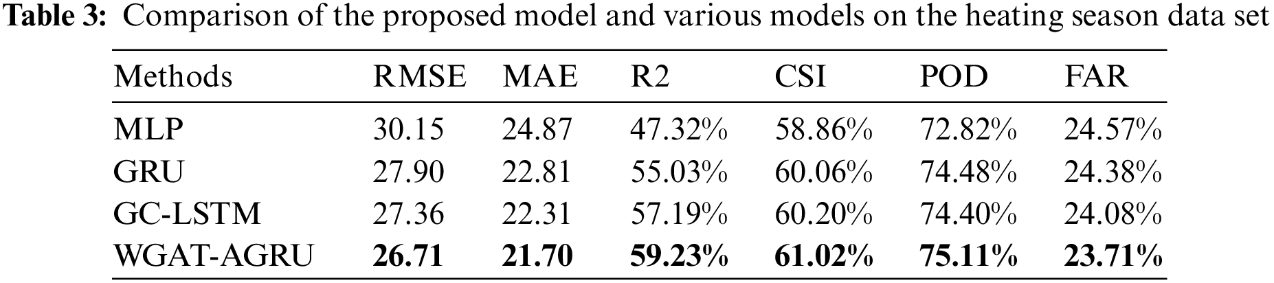
Fig. 4 shows more visually the multi-step PM2.5 concentration prediction capability of the comparison models on the heating season data set, taking Xi’an as an example. The prediction result of the GC-LSTM is similar to the prediction result of the WGAT-AGRU. They both achieve better prediction results than the other two models, GRU and MLP. However, comparing the prediction results of WGAT-AGRU and GC-LSTM, it can be found that the concentration curve predicted by WGAT-AGRU fits the true value of the change better. For example, WGAT-AGRU performs better for the slightly decreasing trend of PM2.5 concentration at the 10-time step, 30-time step, and 40-time step.

Figure 4: Comparison of performance evaluation metrics between different model models on the heating season data set (time step of 24 h, taking Xi’an as an example)

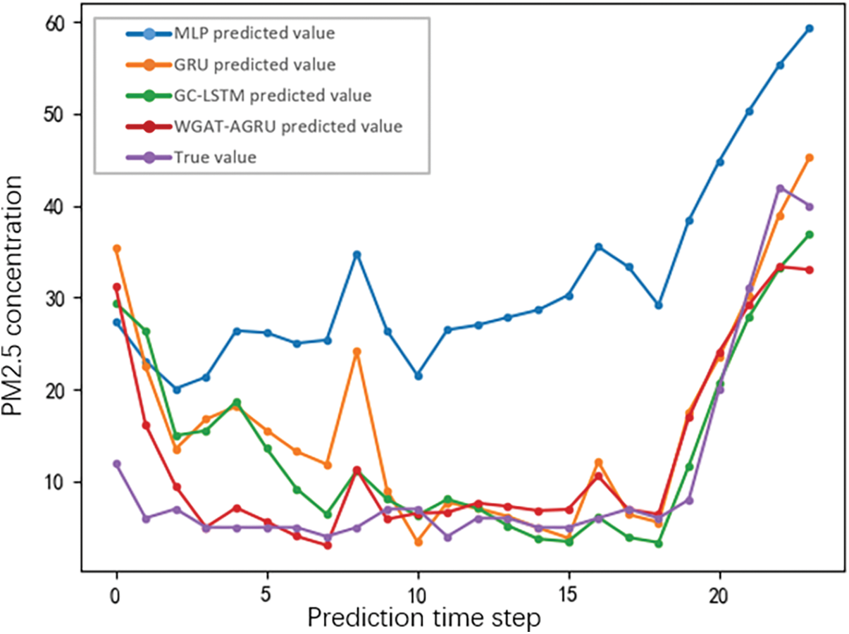
Figure 5: Long-term (72 h) predictions of PM2.5 concentrations from contrasting model models (taking Beijing as an example)

To evaluate the long-term prediction performance of the prediction models, experiments were conducted at different prediction time steps, including 24, 36, and 48 h in this paper. The long-term PM2.5 concentration prediction performance of the models was compared by analyzing the degree of decay of the PM2.5 concentration prediction accuracy of each model with the increase of the prediction step. The experimental results are shown in Table 2. And we can see that the experimental metrics of the proposed model are optimal at each prediction step.

The prediction results of PM2.5 concentration for the next 72 h and the RMSE variation with the prediction step from each model with prediction steps are shown in Figs. 5 and 6. As we can see that the WGAT-AGRU model still maintains an excellent fitting ability for PM2.5 concentration prediction in a long prediction time, and can accurately capture the trend of PM2.5 concentration compared with other prediction models.

Figure 6: Comparison model RMSE variation with prediction time step (taking Beijing as an example)

4.3.2 Validity Analysis

In order to verify the effectiveness of each module of our prediction model, ablation experiments are conducted on the full dataset. The validity of the PM2.5 directed flow graph structure, spatial correlation feature extraction module, and spatiotemporal fusion prediction module on the model are analyzed in this paper, respectively.

The traditional PM2.5 spatial correlation graph DG-INPUT constructs an adjacency matrix by determining whether the distance between city vertices exceeds the threshold and whether the edge weight is the reciprocal of the distance between cities. DG-INPUT and the flow graph FG-INPUT proposed in this paper are used as inputs for experiments on the full data set, respectively, with the same prediction time step set to 24 h. The results are shown in Table 4 (different graph structure input modules). We can see from the result that FG-INPUT improves the model prediction accuracy with the minimum RMSE and MAE because it simulates the impact of inter-city PM2.5 flow transmission well.

To verify the effectiveness of the spatial correlation feature extraction module in the model, WGAT is replaced with the fully connected network (FC), and ablation weight aggregation component (GAT), ablation graph attention component (GNN), respectively. And they are combined with AGRU. The experiments on the full data set are conducted and the prediction step size is uniformly set to 24 h. The results are shown in Table 4 (different spatial correlation feature extraction modules). We can see that the combination of WGAT can effectively improve the prediction result of the model.

To analyze the effectiveness of the spatiotemporal fusion prediction module, WGAT is combined with the fully connected network (FC), ablation temporal attention component (GRU), and the spatiotemporal fusion prediction module (AGRU) of this paper, respectively. Three prediction steps of 24, 36, and 48 h are set, to analyze the effects of each component above on the multi-step prediction of PM2.5 concentration. The experimental results are shown in Table 5. The proposed model WGAT-AGRU achieves the best results in most cases.

4.3.3 Discussion

In this paper, the proposed model WGAT-LSTM with fused spatiotemporal features achieves the best result in most cases. It can be seen from Fig. 3, WGAT-AGRU performs better on the full data set compared with MLP. The MLP model cannot capture the time-dependent relationship, and it cannot predict such drastic changes, and is a poor fit for the peak PM2.5 concentration. While the model proposed in this paper can cope with this situation well and predict the concentration change trend more accurately. And WGAT-AGRU can capture the directional PM2.5 flow through the PM2.5 directed flow graph. GC-LSTM is a graph convolutional neural network that extracts the spatial features between city vertices in the graph structure and achieves spatiotemporal prediction by combining it with LSTM. Thus the prediction result of GC-LSTM is similar to the prediction result of the WGAT-AGRU model. However, during the heating season, when more coal is burned in northern cities in China and the prevailing north wind makes the inter-city PM2.5 concentration more affected by wind propagation, WGAT-AGRU achieves better results as shown in Figs. 4c and 4d. It can be inferred that extracts the PM2.5 spatial flow feature between city vertices in the PM2.5 flow map through WGAT. By analyzing the multi-step prediction ability of the model, it can be found that WGAT-AGRU has better prediction ability when the model is forecasting for a long time. FC cannot capture long-term time dependencies leading to poorer prediction results. When the predicted step size is 24 h, which is the single step length, our multi-step prediction model does not fully reflect the advantages as shown in Table 5 (prediction time step = 24 h).

5  Conclusion

5.1 Conclusion

The existing PM2.5 concentration prediction methods ignore the directionality of PM2.5 flow between cities when constructing spatial correlation maps, and the accuracy of multi-step prediction is low. In this paper, a PM2.5 concentration prediction model WGAT-AGRU integrating spatial and temporal features is constructed and geographic and meteorological data is introduced into the graph structure to construct a PM2.5 directional flow graph to realize the simulation of inter-city PM2.5 flow transmission. Prediction can focus on the key time step information, thus improving the accuracy of the PM2.5 prediction model in multi-step prediction. The comparison experiments with other models on the KnowAir dataset are conducted. The experimental findings indicated that the WGAT-AGRU model is superior to other models in predicting PM2.5 concentration.

5.2 Limitations and Future Work

There are still some limitations in this research. In this paper, the PM2.5 spatial correlation graph is mainly constructed based on the longitude, latitude, altitude, and wind direction data of the cities, and the edge weight is calculated by a simple diffusion transfer model. However, the spatial flow of PM2.5 is more complex. In addition, the PM2.5 concentration prediction model in the paper realizes multi-step prediction of future PM2.5 concentration through continuous iteration. This recursive multi-step prediction strategy makes the prediction error accumulate with the increase of the prediction time step, so it is impossible to predict the long-term PM2.5 concentration.

In the future, we will consider introducing more external features to further optimize the construction of the adjacency matrix of the PM2.5 spatial correlation graph and the calculation of edge weight, to more accurately simulate the flow and transmission of PM2.5 at the spatial level. In addition, optimize the prediction model structure for the multi-step prediction task of PM2.5 concentration, and explore the use of a structure such as the Seq2Seq model to solve the multi-step prediction problem.

Acknowledgement: The authors would like to express their gratitude to Central South University for the financial support through Central South University Research Programme of Advanced Interdisciplinary Studies (2023QYJC041).

Funding Statement: This work was supported by Central South University Research Programme of Advanced Interdisciplinary Studies (2023QYJC041).

Conflicts of Interest: The authors declare that they have no conflicts of interest to report regarding the present study.

References

1. Y. J. Lin, N. Mago, Y. Gao, Y. G. Li, Y. Y. Chiang et al., “Exploiting spatiotemporal patterns for accurate air quality forecasting using deep learning,” in Proc. of the 26th ACM SIGSPATIAL Int. Conf. on Advances in Geographic Information Systems, New York, NY, USA, pp. 359–368, 2018. [Google Scholar]

2. Y. G. Li, R. Yu, C. Shahabi and Y. Liu, “Diffusion convolutional recurrent neural network: Data-driven traffic forecasting,” in Proc. of the 6th Int. Conf. on Learning Representations, Vancouver, BC, Canada, pp. 1–16, 2018. [Google Scholar]

3. Y. L. Qi, Q. Li, H. Karimiana and D. Liu, “A hybrid model for spatiotemporal forecasting of PM2.5 based on graph convolutional neural network and long short-term memory,” Science of the Total Environment, vol. 664, pp. 1–10, 2019. [Google Scholar] [PubMed]

4. X. B. Jin, N. X. Yang, X. Y. Wang, Y. T. Bai, T. L. Su et al., “Integrated predictor based on decomposition mechanism for PM2.5 long-term prediction,” Applied Sciences, vol. 9, no. 21, pp. 1–14, 2019. [Google Scholar]

5. L. Y. Zhang, J. Lin, R. Z. Qiu, X. S. Hu, H. H. Zhang et al., “Trend analysis and forecast of PM2.5 in Fuzhou, China using the ARIMA model,” Ecological Indicators, vol. 95, pp. 702–710, 2018. [Google Scholar]

6. V. Venkataraman, S. Usmanulla, A. Sonnappa, P. Sadashiv, S. S. Mohammed et al., “Wavelet and multiple linear regression analysis for identifying factors affecting particulate matter PM2.5 in Mumbai City, India,” International Journal of Quality & Reliability Management, vol. 36, no. 10, pp. 1750–1783, 2019. [Google Scholar]

7. A. Tai, L. Mickley, D. Jacob, E. Leibensperger, L. Zhang et al., “Meteorological modes of variability for fine particulate matter (PM2.5) air quality in the United States: Implications for PM2.5 sensitivity to climate change,” Atmospheric Chemistry And Physics, vol. 12, no. 6, pp. 3131–3145, 2012. [Google Scholar]

8. A. Shamsoddini, M. R. Aboodi and J. Karami, “Tehran air pollutants prediction based on random forest feature selection method,” International Archives of the Photogrammetry, Remote Sensing & Spatial Information Sciences, vol. 42, pp. 483–488, 2017. [Google Scholar] [PubMed]

9. Y. H. Dong, H. Wang, L. Zhang and K. Zhang, “An improved model for PM2.5 inference based on support vector machine,” in 2016 17th IEEE/ACIS Int. Conf. on Software Engineering, Artificial Intelligence, Networking and Parallel/Distributed Computing (SNPD), Shanghai, China, pp. 27–31, 2016. [Google Scholar]

10. P. Wang, H. Zhang, Z. D. Qin and G. S. Zhang, “A novel hybrid-Garch model based on ARIMA and SVM for PM2.5 concentrations forecasting,” Atmospheric Pollution Research, vol. 8, no. 5, pp. 850–860, 2017. [Google Scholar]

11. G. Asadollahfardi, M. Madinejad, S. H. Aria and V. Motamadi, “Predicting particulate matter (PM2.5) concentrations in the air of Shahr-e Ray City, Iran, by using an artificial neural network,” Environmental Quality Management, vol. 25, no. 4, pp. 71–83, 2016. [Google Scholar]

12. X. Mao, T. Shen and X. Feng, “Prediction of hourly ground-level PM2.5 concentrations 3 days in advance using neural networks with satellite data in eastern China,” Atmospheric Pollution Research, vol. 8, no. 6, pp. 1005–1015, 2017. [Google Scholar]

13. I. G. McKendry, “Evaluation of artificial neural networks for fine particulate pollution (PM10 and PM2.5) forecasting,” Journal of the Air & Waste Management Association, vol. 52, no. 9, pp. 1096–1101, 2002. [Google Scholar]

14. B. T. Ong, K. Sugiura and K. Zettsu, “Dynamic pre-training of deep recurrent neural networks for predicting environmental monitoring data,” in 2014 IEEE Int. Conf. on Big Data (Big Data), Washington, DC, USA, pp. 760–765, 2014. [Google Scholar]

15. Y. T. Tsai, Y. R. Zeng and Y. S. Chang, “Air pollution forecasting using RNN with LSTM,” in 2018 IEEE 16th Int. Conf. on Dependable, Autonomic and Secure Computing, 16th Int. Conf. on Pervasive Intelligence and Computing, 4th Int. Conf. on Big Data Intelligence and Computing and Cyber Science and Technology Congress (DASC/PiCom/DataCom/CyberSciTech), Athens, Greece, pp. 1074–1079, 2018. [Google Scholar]

16. M. Krishan, S. Jha, J. Das, A. Singh, M. K. Goyal et al., “Air quality modelling using long short-term memory (LSTM) over NCT-Delhi, India,” Air Quality, Atmosphere & Health, vol. 12, no. 8, pp. 899–908, 2019. [Google Scholar]

17. D. Chi, Q. Huang and L. Z. Liu, “Dissolved oxygen concentration prediction model based on WT-MIC-GRU—a case study in dish-shaped lakes of Poyang Lake,” Entropy, vol. 24, no. 4, pp. 1–18, 2022. [Google Scholar]

18. A. Chakma, B. Vizena, T. Cao, J. Lin and J. Zhang, “Image-based air quality analysis using deep convolutional neural network,” in 2017 IEEE Int. Conf. on Image Processing (ICIP), Beijing, China, pp. 3949–3952, 2017. [Google Scholar]

19. J. Ma, K. Li, Y. H. Han, P. F. Du and J. Y. Yang, “Image-based PM2.5 estimation and its application on depth estimation,” in 2018 IEEE Int. Conf. on Acoustics, Speech and Signal Processing (ICASSP), Calgary, AB, Canada, pp. 1857–1861, 2018. [Google Scholar]

20. L. Cheng, L. Li, S. Li, S. Ran, Z. Zhang et al., “Prediction of gas concentration evolution with evolutionary attention-based temporal graph convolutional network,” Expert Systems with Applications, vol. 200, no. 7, pp. 116944, 2022. [Google Scholar]

21. C. F. F. Karney, “Algorithms for geodesics,” Journal of Geodesy, vol. 87, no. 1, pp. 43–55, 2013. [Google Scholar]

22. K. F. Zhang, X. L. Yang, H. Cao, J. Thé, Z. C. Tan et al., “Multi-step forecast of PM2.5 and PM10 concentrations using convolutional neural network integrated with spatial–temporal attention and residual learning,” Environment International, vol. 171, pp. 107691, 2023. [Google Scholar] [PubMed]