CNN-Based RF Fingerprinting Method for Securing Passive Keyless Entry and Start System

1  Introduction

Modern vehicles are equipped with many advanced technologies to enhance customer convenience. Some examples of these modern vehicles include connected cars and self-driving cars. These advanced vehicles can utilize external communications, such as the internet, to acquire various information and can be operated automatically through autonomous driving systems. Due to the increasing popularity of these convenient features, there has been a rapid rise in attempts to attack vehicle systems. Therefore, developing effective security systems for modern vehicles is crucial to avoid causing substantial financial damage or incidents that may threaten passenger safety. In this paper, we propose a radio frequency (RF) fingerprinting method to protect the passive keyless entry and start system (PKES), which is a widely used primary feature of modern vehicles [1]. The PKES system allows unlocking and starting the vehicle without a physical key. If the RF signal from the keyfob reaches the sensors in the vehicle, the doors are automatically opened, and the engine can be started without user interaction. While this automatic entry system provides many conveniences, it is vulnerable to attacks such as relay attacks. According to reports in [2–5], many relay attacks on passive or remote keyless entry systems are feasible, including two types of attacks: single-band and dual-band relay attacks.

In a scenario where a vehicle sends a low-frequency (LF) signal to sense the keyfob nearby, if the keyfob is out of range and cannot receive the LF signal, it will not respond with any radio frequency signal, such as an ultra-high frequency (UHF) signal [6]. In a single-band relay attack, the RF signal is amplified to extend its reach, causing the keyfob to respond to the amplified LF signal, allowing the attacker to operate the vehicle.

In a dual-band relay attack, two relay stations establish a higher frequency band link and extend the original LF signal’s reach. Two stations are located near the vehicle and keyfob, respectively. The vehicle-side station receives the LF signal from the vehicle first, converts it to the higher frequency signal, and sends it to the key-side station. The key-side station then converts the delivered signal back to the LF signal and sends it to the key. The keyfob receives the LF signal transmitted by the key-side station and responds with the UHF signal directly to the vehicle sensor or through the established link created by the attacker.

Our method prevents attacks on PKES systems by verifying the authenticity of signals sent by RF transmitters. For achieving device authentication, the method first defines the unique fingerprints of the signal sent by a legitimate transmitter. It uses them to train a machine learning-based device identification model for authenticating anonymous signals in the future. Our method utilizes cepstral coefficient features to represent the unique spectral characteristics of audio signals. The cepstral coefficient feature has been widely used in speech processing because it can effectively capture the significant frequency components of signals and reduce the influence of irrelevant noise and other distortions. Cepstral coefficient features can define the unique attributes of signals in the higher frequency band used in PKES, thereby providing the potential to identify the distinct characteristics of RF signals. Although similar approaches [7,8] have been proposed, most existing approaches focus on applying only well-known features, such as Mel-Frequency Cepstral Coefficients (MFCC). Unlike the existing approaches, among many cepstral coefficient feature types, we try to find the key feature useful for RF fingerprinting while finding a way to process the cepstral coefficient feature using machine learning models.

In the evaluation phase, we collected numerous RF signals from various RF transmitters to demonstrate the effectiveness of our method in identifying devices through the analysis of cepstral coefficient features. In addition, we experimented with evaluating the usefulness of various cepstral coefficients such as Mel-Frequency Cepstral Coefficients (MFCC), Inverse MFCC (IMFCC), Bark-Frequency Cepstral Coefficients (BFCC), Gammatone-Frequency Cepstral Coefficients (GFCC), and Linear-Frequency Cepstral Coefficients (LFCC). Lastly, we also compared our performance with the existing approaches similar to our method.

The remainder of the paper is structured as follows: Sections 2 and 3 review the relevant literature and provide background information on our research. Section 4 details the proposed method’s overall architecture and its components. In Section 5, we present the experimental results to demonstrate the effectiveness of our method, and in Section 6, we summarize our research and outline future directions for this ongoing study.

2  Related Work

In this section, the previous approaches related to radio frequency (RF) fingerprinting for security are explained in turn. Various researchers have studied wireless signal fingerprinting for device identification or authentication. The authors of [9] proposed a method that utilizes wireless signal noise data to pair wearable devices without any intervention. The framework introduced in [10] employs wireless signal fingerprinting embeddings to improve individual identification performance, and the Study [11] introduced a method that applies wireless signal fingerprinting to the physical layer of fixed Internet of Things (IoT) devices to provide enhanced security. In [12], a method to explore the damage of transmitters and receivers in narrowband systems is presented, and the effects of the method on radio frequency fingerprint identification (RFFI) are simulated.

In addition to these previous works, studies on wireless signal fingerprinting for device authentication using deep learning have also been conducted. Bihl et al. [13] investigated feature selection methods for wireless signal fingerprinting and proposed the multiple discriminant analysis (MDA) loadings fusion method to improve the accuracy of MDA-based classifiers. In addition, there is an approach [14] to IoT terminal authentication using a convolutional neural network (CNN) model and a two-dimensional feature called Differential Constellation Trace Figure (DCTF) to define the RF fingerprint. Similarly, Li et al. [15] used a deep learning method and proposed a fine-tuning approach to update the neural network model with new data, improving accuracy. Some approaches are similar to our method. For example, Diao et al. [7] proposed an MFCC-based drone authentication method using an acoustic fingerprint and evaluated the performance using various machine-learning models. The authors found that Quadratic Discriminant Analysis (QDA) was the best model for effectively analyzing MFCC features.

Similarly, Kılıç et al. [8] developed a drone classification method that analyzed spectral features, including MFCC and LFCC, using the support vector machine (SVM) for authenticating pre-registered drones. Our method differs from these previous approaches. We evaluated many kinds of the cepstral coefficient feature to choose the best effective feature and eventually utilized the GFCC feature to define the RF fingerprint. Moreover, in [7,8], no consideration is given to developing a model that can learn the spatial information present in the cepstral coefficient features. In our experiment, we demonstrated the effectiveness of the GFCC and CNN model inductively and compared our method’s performance with those of previous approaches. We found that the CNN model is useful for analyzing the GFCC feature for device authentication.

Additionally, there are some studies on radio frequency fingerprinting methods for wireless attack detection. Maleki et al. [16] presented an analysis of radio frequency identification (RFID) technology’s replication detection mechanisms and their characteristics. In [17], a forensics framework for detecting fake base station (FBS) attacks is presented. The radio frequency signal fingerprints are generated based on modulation errors, instantaneous frequency, and phase differences and are used for detecting FBS attacks. These studies also emphasize that the distinctive characteristics of radio frequency signals can be defined and utilized in various scenarios. Therefore, as suggested in [16,17], we anticipate that our method could be applied to various security systems.

3  Our Proposed Method

Our suggested approach takes advantage of the distinct characteristic information presented in the radio frequency (RF) signals a legitimate keyfob produces to authenticate its RF transmitter. The unique feature used as the RF fingerprint arises from hardware imperfections during manufacturing [18]. Although manufacturers strive to create identical RF transmitters, physical differences between various hardware components are inevitable. Furthermore, these physical distinctions are manifested in the RF signal. Hence, our method focuses on identifying the unique characteristics of the RF signal as fingerprints and verifying whether the transmitted signal originates from a legitimate device. This approach enables the differentiation between a genuine RF transmitter and an abnormal one, which might be a device used by an attacker for a relay attack.

Fig. 1 illustrates the comprehensive architecture of the proposed method, which consists of two primary components: the fingerprint extraction component and the device identification component. The fingerprint extraction component first accepts an ultra-high frequency (UHF) signal with a frequency of 433 MHz and produces a unique cepstral coefficient feature. The cepstral coefficient feature is used as the RF fingerprint and is derived from the spectral representation of a signal. It provides a compact representation that captures the main characteristics of the spectral envelope while being less susceptible to noise. The fingerprint extraction component generates the cepstral coefficient feature of the input signal through a series of six steps: pre-emphasis, framing, windowing, fast Fourier transformation (FFT), filter bank application, and discrete cosine transformation (DCT). On the other hand, the device identification component associates the cepstral coefficient feature with a specific device. A convolutional neural network (CNN) is employed to perform the identification process. The CNN outputs the Softmax probabilities for the registered normal devices, and based on these probabilities, the input signal is classified by the component as belonging to a specific device. The device with the highest Softmax probability above a pre-specified threshold is selected by the component as the predicted device. If none of the devices’ probabilities exceed the threshold, the component concludes that the input signal is from an abnormal device.

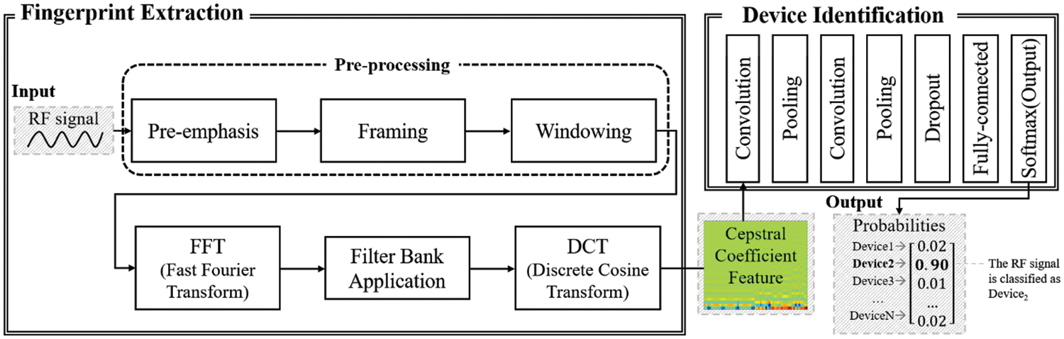
Figure 1: The overall architecture of our proposed method

3.1 Fingerprint Extraction Component

The fingerprint extraction component conducts seven steps to extract the cepstral coefficient feature from the provided RF signal. Three pre-processing steps-pre-emphasis, framing, and windowing-are executed to amplify the original signal and divide the entire signal into frames, which serve as the fundamental units for refinement in subsequent processes. After this, the frames are transformed using the Fourier transform to convert them from the time domain to the frequency domain. The power spectrum for each frame is then calculated from the Fourier coefficients. The power spectrum represents the signal’s power across different frequencies, and it shows how much of the signal’s energy is distributed across different frequency bands. Next, filter banks are determined based on the power spectrum, and the Discrete Cosine Transform (DCT) is applied to the filter banks to ultimately obtain the cepstral coefficients. Once the fingerprint extraction component completes all the steps, the device identification component uses the extracted features to train the convolutional neural network or analyzes the features from a random signal targeted for authentication.

3.1.1 Pre-Emphasis

One of the initial steps in the feature extraction process is to apply a pre-emphasis filter to the signal. Specifically, the pre-emphasis filter boosts the amplitudes of high-frequency components of the signal while reducing the amplitudes of low-frequency components. This is done by applying a filter that amplifies the high-frequency components and attenuates the low-frequency components. By doing so, the pre-emphasis filter helps to balance the signal’s frequency spectrum, which can improve the quality of the signal and make it easier to analyze using techniques such as the Fourier transform. Additionally, the pre-emphasis filter can help reduce certain types of noise that may be present in the signal, such as low-frequency noise often caused by electrical interference. Eq. (1) described the pre-emphasis process mathematically.

y[n]=x[n]−a×x[n−1](1)

1

where x[n] is the input signal at time n, y[n] is the pre-emphasized output signal at time n, and a is a pre-emphasis coefficient.

3.1.2 Framing

The framing process involves splitting the entire signal into short-time frames of a fixed size, with each frame being slightly offset from the previous one by a value called the stride. Overlapping frames in this way ensure that each frame contains some of the same information as the previous frame, which can help to reduce the impact of abrupt changes in the signal’s frequency content. This is particularly important when applying techniques such as the Fourier transform, as it can help to prevent the loss of important frequency information over time. By processing each frame separately and concatenating the adjacent frames, it is possible to obtain a good approximation of the frequency contours of the original signal.

3.1.3 Windowing

Windowing is an important step in the feature extraction process that is used to reduce the noise and artifacts that can be introduced during the Fourier transform. In this step, a hamming window function is applied to each frame of the signal that was previously split from the original signal. By applying the Hamming window function to each frame, the left and right end regions of the frame are smoothed while maintaining the overall shape of the frame. This helps to remove unnecessary high-frequency components of the frame signal. As a result, the windowing process can enhance the quality of the signal and make it easier to analyze. It is important to note that the choice of window function can have a significant impact on the quality of the resulting signal. In this case, the Hamming window function is used due to its desirable properties, such as good spectral resolution and low spectral leakage. It is noted that windowing and framing are conducted simultaneously, and the equation for the operation is described in Eq. (2).

x[n]=w[n]×x(t(nT+mΔ))(2)

2

where x[n] is the signal in the nth frame, w[n] is the window function applied to the nth frame, t is a continuous time variable, and m is an integer index that varies from 0 to M−1, where M is the number of samples in each frame.

3.1.4 FFT(Fast Fourier Transform)

The fast Fourier transform (FFT) is an efficient algorithm used to compute the discrete Fourier transform (DFT) of a signal, which converts a signal from its time domain to a representation in the frequency domain. This transformation is achieved by decomposing the signal into its constituent components of different frequencies. Unlike the traditional DFT, which has a computational complexity of n2, the FFT algorithm factorizes the DFT matrix into a product of sparse factors, resulting in a computational complexity of only nlog⁡n. This significantly reduces the computational load required to perform the transformation, making it a highly effective tool for analyzing signals with large amounts of data. The mathematical description for the FFT is shown in Eq. (3).

x[k]=∑n=0N−1⁡x[n]×exp⁡(−j2πkn/N)(3)

3

where x[k] is the kth frequency component, j is the imaginary unit, and k=0, 1, … , N−1.

3.1.5 Applying Filter Bank

A filter bank is an array of bandpass filters that separates the original signal into multiple components, with each component carrying a single frequency sub-band. The filter bank helps to decompose the signal into its constituent parts, making it easier to analyze and extract relevant features. Different types of filters can be used in a filter bank, each with its characteristics. These filters are designed to amplify specific frequency regions of the signal more than others based on the desired frequency response. In our research, we examined the effectiveness of six representative filters in terms of device authentication. These included filters for the mel scale, inverse mel scale, linear scale, and other types. Each filter was selected based on its ability to effectively extract unique characteristics of the RF signal and improve the accuracy of device authentication. The choice of filter type and parameters can have a significant impact on the quality and accuracy of the extracted features. Therefore, it is important to carefully select the appropriate filter type and design its parameters according to the specific requirements of the application. The mathematical description for the filter bank application is described in Eq. (4).

Spectogram=PowSpectrums⋅FbankT=[a11⋯an⋮⋱⋮am1⋯amn][b11⋯b1n⋮⋱⋮br1⋯brn]T(4)

4

where PowSpectrums means power spectrums consisting of magnitude, a, Fbank means filter bank consisting of filter weights b, m is the number of frames, n is the number of frequencies in frequency bin, and r is the number of filters.

Mel Scale Filter Bank: The cepstral coefficient feature obtained through the use of the mel scale filter bank is known as the mel frequency cepstral coefficient (MFCC) [19]. The mel scale filter bank utilizes a set of mel scale filters, which are triangular filters that increase and decrease linearly from the center of the filter. The Mel scale filter bank is designed to more closely approximate the human auditory system’s response to sound compared to linearly spaced frequency bands. This is because the human auditory system has greater sensitivity to changes in lower frequencies than higher ones. By using the mel scale filter bank, the lower frequency regions of the power spectrum are amplified since there are more filters in the lower frequency range compared to the higher frequency range. The example of the mel scale filter bank is shown in Fig. 2. The graph in the figure shows the normalized amplitude of impulse response of each mel scale filter along the frequency. It should be noted that in our implementation, we utilized normalized amplitudes between the range of 0 to 1, up to a frequency of 10 MHz, which is half of the sampling rate as specified by the Nyquist theorem [20].

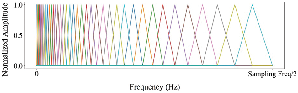
Figure 2: The example of the mel scale filter bank (The x-axis shows frequency in 1 Hz scale, and the y-axis shows the normalized impulse response amplitude, ranging from 0 to 1 as a real value)

Inverse Mel Scale Filter Bank: The cepstral coefficient feature obtained using the inverse mel scale filter bank is called inverse mel frequency cepstral coefficient (IMFCC) [21]. The inverse mel scale filter bank is made up of inverse mel scale filters, which are triangular filters with a similar shape to mel scale filters. However, while mel scale filters are concentrated in the lower frequency region of the spectrum, inverse mel scale filters are concentrated in the higher frequency region. The example of the inverse mel scale filter bank is illustrated in Fig. 3. The graph in the figure shows the normalized amplitude of impulse response of each mel scale filter along the frequency. It should be noted that we utilized normalized amplitudes ranging from 0 to 1 and up to 10 MHz, which is half of the sampling rate as specified by the Nyquist theorem in our approach [20]. This technique is useful for feature extraction in applications where the high-frequency components of the signal are particularly important, such as in the identification of specific electronic devices based on their RF signals.

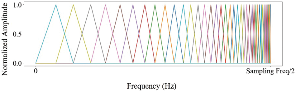
Figure 3: The example of the inverse mel scale filter bank (The x-axis shows frequency in 1 Hz scale, and the y-axis shows the normalized impulse response amplitude, ranging from 0 to 1 as a real value)

Linear Scale Filter Bank: The cepstral coefficient feature extracted using the linear filter bank is called the linear frequency cepstral coefficient (LFCC) [22]. Linear filter banks are comprised of triangular filters similar to those found in mel scale and inverse mel scale filter banks. However, unlike these other types of filter banks, the linear filter bank evenly distributes the triangular filters across the frequency spectrum. This means that there is no emphasis on a particular frequency range. Fig. 4 depicts the example of the linear frequency filter bank. The graph in the figure shows the normalized amplitude of impulse response of each mel scale filter along the frequency. It should be noted that we utilized normalized amplitudes ranging from 0 to 1 and up to 10 MHz, which is half of the sampling rate in our implementation.

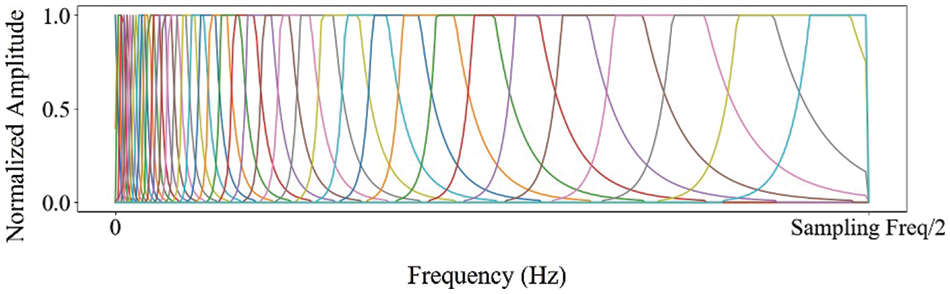
Figure 4: The example of the linear scale filter bank (The x-axis shows frequency in 1 Hz scale, and the y-axis shows the normalized impulse response amplitude, ranging from 0 to 1 as a real value)

Bark Scale Filter Bank: The cepstral coefficient feature obtained using the bark scale filter bank is called the bark frequency cepstral coefficient (BFCC) [23]. The bark scale filter bank uses the smoothed trapezoidal filters to process each the power spectrum of the separated sub-band in a non-linear manner, closely mimicking the frequency response of the human auditory system. Unlike uniform filters, the bark scale filter reaches the converging region faster, making it more suitable for capturing the non-linearities of the human ear. Fig. 5 depicts the example of the bark scale filter bank. The graph in the figure shows the normalized amplitude of impulse response of each bark scale filter along the frequency. It should be noted that we utilized normalized amplitudes ranging from 0 to 1 and up to 10 MHz, which is half of the sampling rate in our implementation.

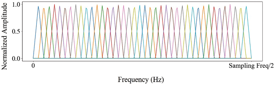
Figure 5: The example of the bark scale filter bank (The x-axis shows frequency in 1 Hz scale, and the y-axis shows the normalized impulse response amplitude, ranging from 0 to 1 as a real value)

Gammatone Filter Bank: The cepstral coefficient feature using the gammatone filter bank is known as the gammantone frequency cepstral coefficient (GFCC) [24] and has been used in various applications, including speech and audio signal processing. One notable characteristic of the gammatone filter bank is that the shape of the gammatone frequency filter is determined by an impulse response that is the product of a gamma distribution and sinusoidal tone. This results in a filter that increases or decreases rapidly at the center frequency of the filter. While the magnitude profile of the gammatone filter is similar to that of the bark scale filter, the behavior of the filter at the center frequency is different. The gammatone filter bank divides the power spectrum into multiple sub-bands, with each sub-band being processed by a gammatone filter. Fig. 6 shows the example of the gammatone filter bank and its corresponding gammatone filters. The graph in the figure shows the normalized amplitude of impulse response of each bark scale filter along the frequency. It should be noted that in our implementation, we utilized normalized amplitudes between the range of 0 to 1, up to a frequency of 10 MHz, which is half of the sampling rate as specified by the Nyquist theorem [20].

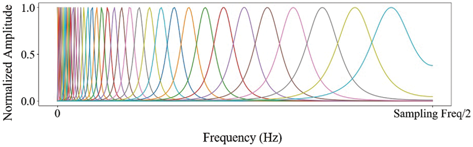
Figure 6: The example of the gammatone filter bank (The x-axis shows frequency in 1 Hz scale, and the y-axis shows the normalized impulse response amplitude, ranging from 0 to 1 as a real value)

3.1.6 DCT(Discrete Cosine Transform)

The discrete cosine transform (DCT) is an essential step in the feature extraction process. The DCT is a mathematical technique used to convert a signal from the time domain to the frequency domain by correlating the values of the signal’s spectrum. This process results in a representation of the spectral properties of the signal, which can be used for further analysis. The DCT is similar to the inverse Fourier transform, but it is specifically designed to create a compact representation of the signal in terms of its cosine basis functions. By using the DCT, we can obtain a compact and efficient representation of the signal that contains only the most relevant information for further analysis. This can help to improve the accuracy and efficiency of the feature extraction. The mathematical description is depicted in Eq. (5).

x[k]=∑n=0N−1⁡x[n]×cos⁡(πk(n+1/2)/N)(5)

5

where x[k] is the kth DCT coefficient of the sequence x[n], and n and k are integer indices ranging from 0 to N−1.

3.2 Device Identification Using Convolutional Neural Network

In the device identification component, the convolutional neural network model shown in Fig. 7 is used to classify the given fingerprint features into the device classes. A convolutional neural network is one of the deep learning methods that simulate the human optic nerve system, and it is widely used in image recognition or vision research. The convolutional neural network can learn the spatial characteristics of the given input and use them to determine the class of the feature input. The cepstral coefficient feature consists of the DCT of the spectral envelopes of many frames, and it has a strong interrelation between each spectral envelope because each frame is overlapped when framing is performed. For this reason, the device identification component uses the convolutional neural network as a classification model.

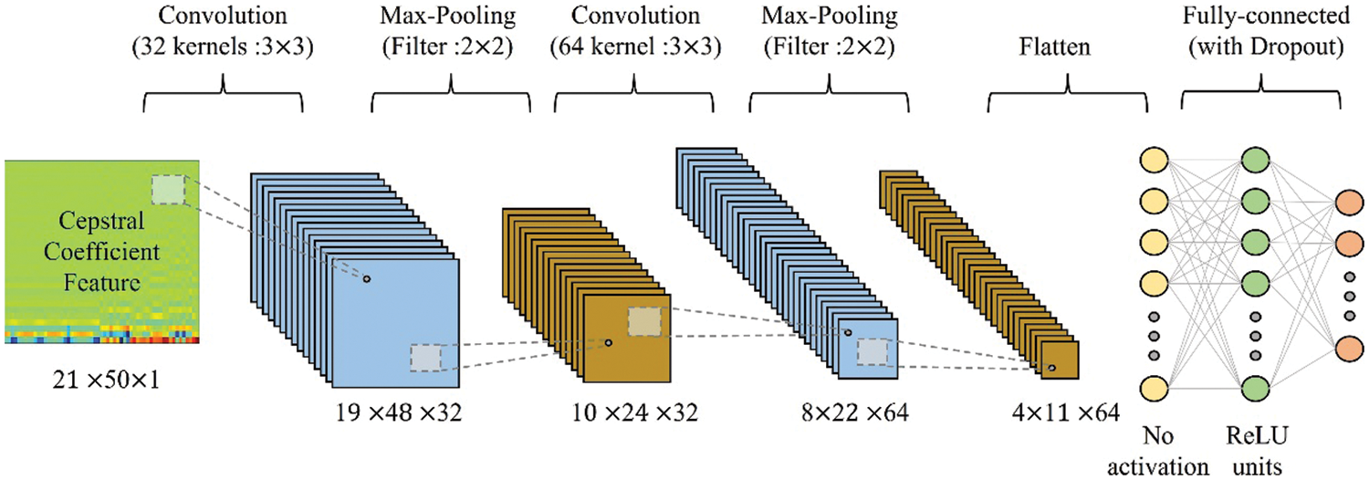
Figure 7: The structure of the convolutional neural network model (The number of frames in a signal is set to 21, and the number of coefficients is set to 50)

The structure and parameters of the model are presented in Table 1 and Fig. 7, respectively. The device identification component of the model consists of two convolution layers, two max-pooling layers, a fully-connected layer, and an output layer. The convolution layers perform a convolution operation on the data using a set of learnable kernel filters to extract increasingly complex features from the data. During the convolution operation, the kernel filters slide over the original data and produce a feature map that represents the spatial relationship between the original data and the filters. In our model, the size of the kernel filters for the convolution is set to 3 × 3. The 3 × 3 kernel size is a common choice for making the feature maps capture local features while maintaining a relatively small receptive field to prevent overfitting.

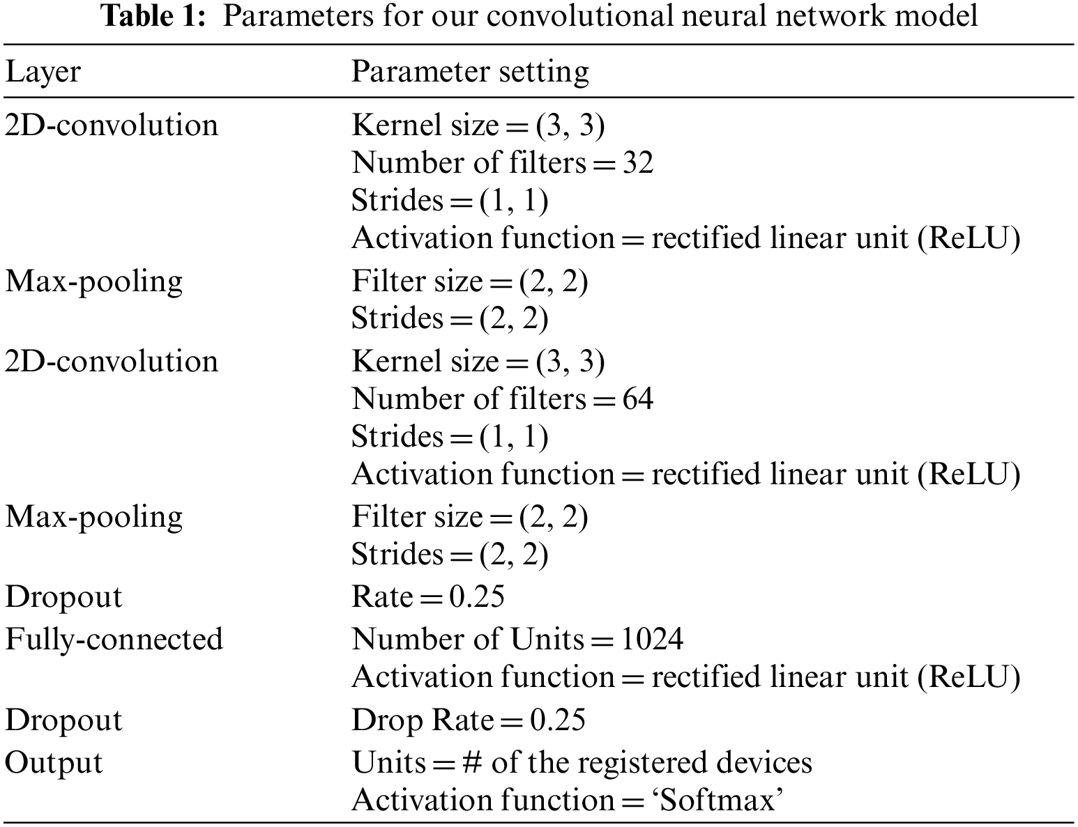
The output feature maps of each convolution layer are then passed through the succeeding max-pooling layers, which reduce the dimensionality of the feature maps by selecting the maximum value within each pooling window. This operation extracts the most relevant information from the feature maps and reduces the number of parameters in the model, thereby reducing overfitting. We chose a max-pooling filter size of 2 × 2, which is relatively small, to avoid excessive information reduction while down-sampling the data.

The output data from the last max-pooling layer is passed to the dropout layer. The dropout layer is also included to prevent overfitting of the model by randomly dropping out some of the neurons during training. The dropout probability was set to 0.25. This value was chosen to strike a balance between reducing overfitting while not dropping out too many neurons, which could reduce the overall performance of the model. After dropping out some neurons, the weighted sum values of the active neurons and the weights are calculated and passed to the fully-connected layer. Then, the Rectified Linear Unit (ReLU) function is applied to introduce non-linearity into the model, and the converted values are processed by the dropout layer again. The values from the active neurons that remain are passed to the output layer, which produces the final classification results using the Softmax function to calculate the probability of the input belonging to each device class.

4  Evaluation

4.1 Experimental Dataset and Parameters

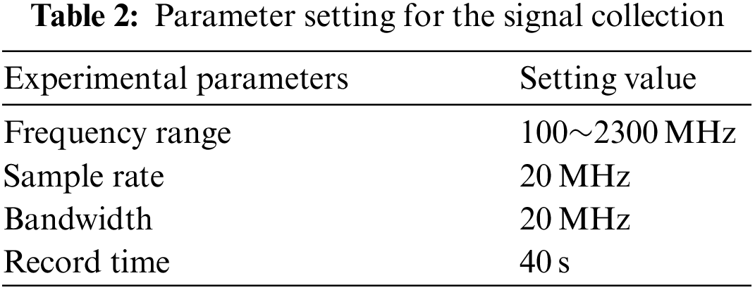
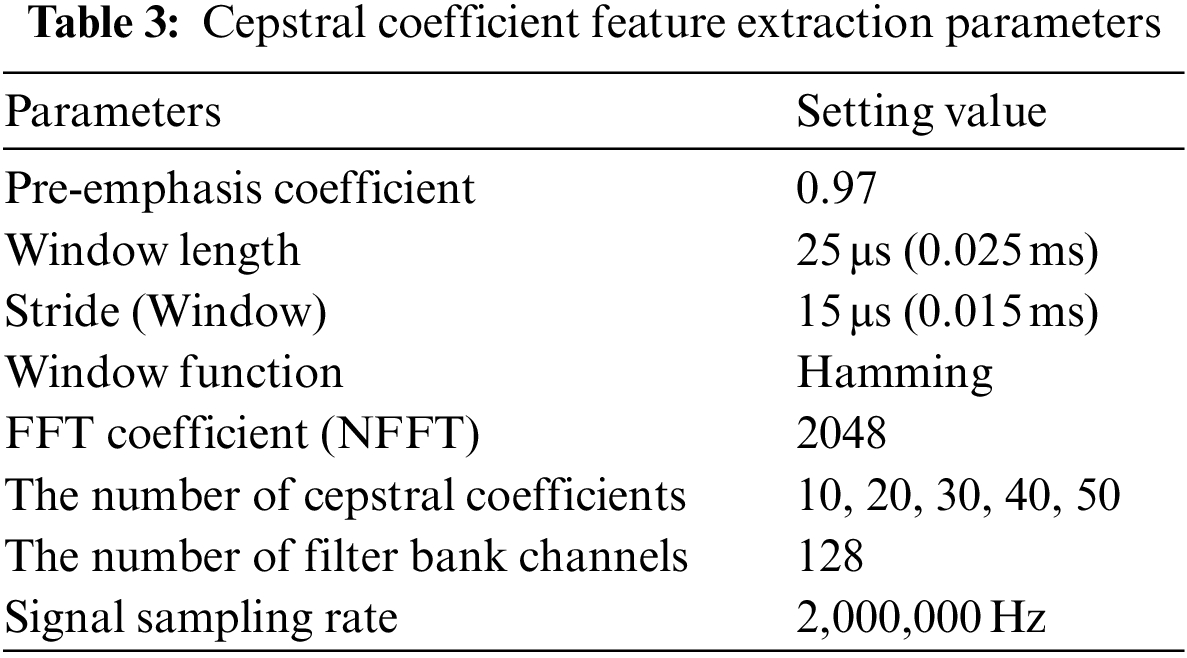
The pictures of the equipment used in the experiment are presented in Fig. 8, and our experimental environment setup is depicted in Fig. 9. We collected experimental data by utilizing seven Arduino Uno boards, each equipped with a different 433 MHz wireless signal transmitter and a HackRF with a radio frequency (RF) antenna to capture the ultra-high frequency (UHF) signal transmitted by each of the transmitters. We used the Arduino Uno boards with RF transmitters to simulate key fobs sending UHF band signals in response to a vehicle-side request to check the proximity of the key fob. Our goal was to check if the transmitted UHF signal came from the normal key fob and not an attacker’s key-side relay station in the event of a dual-band relay attack. In our experiment, we set the sampling rate for signal collecting to 20 MHz, and we extracted the collected UHF signals using the osmocom source module. We set the distance between the UHF transmitters and the HackRF device to 0.5 meters. The length of a signal in time was 0.0034 s on average. We collected 140,000 signal data in total, with 20,000 for each wireless signal transmitter. We split the training and test sets for device identification into 70% and 30% proportions, respectively. More detailed parameter setting information for the signal collection is presented in Table 2. In addition to the experimental parameters, it is important to note that the choice of parameters can have a significant impact on the evaluation result. Table 3 provides a list of the parameter settings used to generate the cepstral coefficient features in the fingerprinting component.

Figure 8: Picture of sample equipment

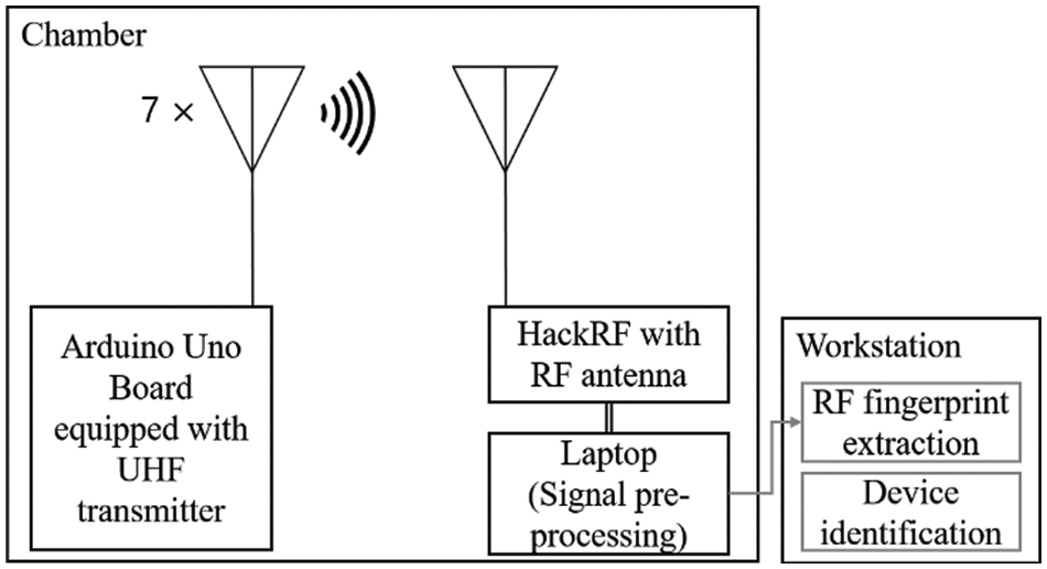
Figure 9: Experimental environment for capturing UHF signals

4.2 The Accuracy Measurement Result for the Device Identification

The effectiveness of our proposed device identification method was evaluated through an experiment. We measured the accuracy of the convolutional neural network and the feed-forward neural network while varying the cepstral coefficient feature used as the input fingerprint for the models, including Mel-Frequency Cepstral Coefficients (MFCC), Inverse MFCC (IMFCC), Bark-Frequency Cepstral Coefficients (BFCC), Gammatone-Frequency Cepstral Coefficients (GFCC), and Linear-Frequency Cepstral Coefficients (LFCC). The feed-forward neural network used in our evaluation consists of seven layers, which can be categorized into three types: input layer, hidden layer, and output layer. The input layer receives the flattened cepstral coefficient feature as the input data, and the hidden layers perform mathematical operations on the input data to extract relevant features and patterns. Each hidden layer contains multiple neurons, and each neuron takes the output from the previous layer and performs a weighted sum of the inputs. The output of each neuron then undergoes the rectified linear unit (ReLU) activation function, which introduces non-linearity into the model. The output layer of the neural network uses the Softmax function to determine the probability of the input data being classified into a specific device class. The model then classifies the input data into the device class with the highest probability that exceeds the pre-defined threshold. If there is no device class with a probability exceeding the threshold, the input data is considered abnormal. The architecture of the feed-forward neural network and its parameter settings are described in Table 4 and Fig. 10.

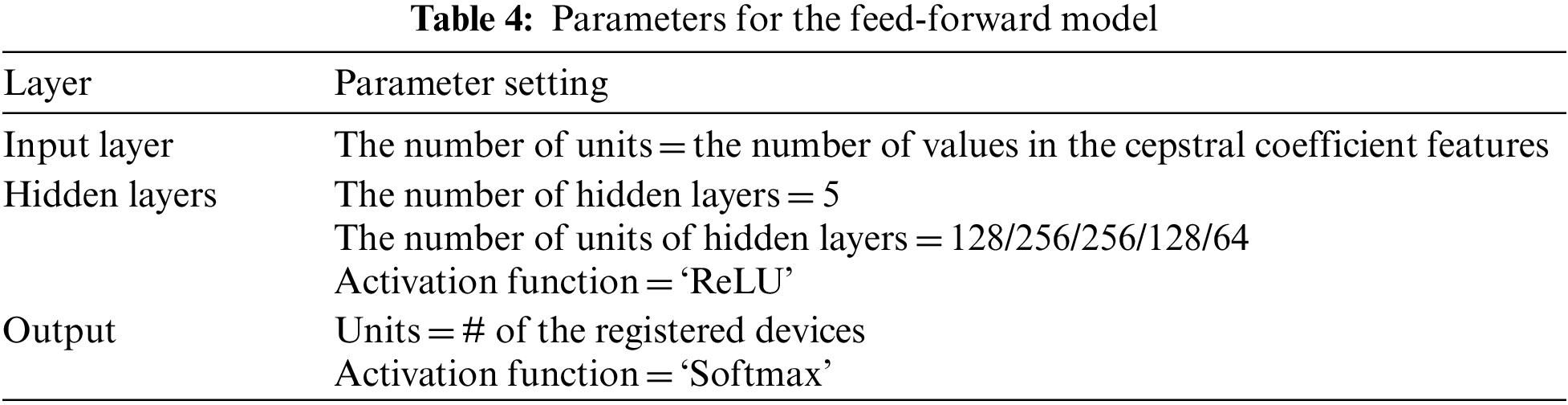
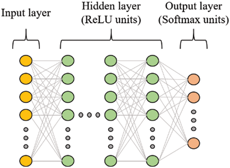
Figure 10: The architecture of the feed-forward neural network

Based on our experimentation, we found that the convolutional neural network model exhibited superior performance compared to the feed-forward neural network model in identifying devices. Tables 5 and 6 show the accuracy results for the feed-forward neural network model and the convolutional neural network model, respectively. The accuracies included in both tables were measured while varying the number of coefficients because the number of coefficients can affect the performance. The number of coefficients determines the amount of information extracted from the signal. More coefficients generally result in a more detailed representation of the signal’s spectral characteristics. Compared to the feed-forward algorithm, the convolutional neural network model produced an average accuracy improvement of 12%. Moreover, in the case of the convolutional neural network model, unlike the feed-forward neural network model, the accuracy values for MFCC, IMFCC, BFCC, GFCC, and LFCC range from 99.32% to 99.99%, 99.93% to 99.90%, 99.94% to 99.99%, 99.98% to 99.99%, and 99.96% to 99.99%, respectively.

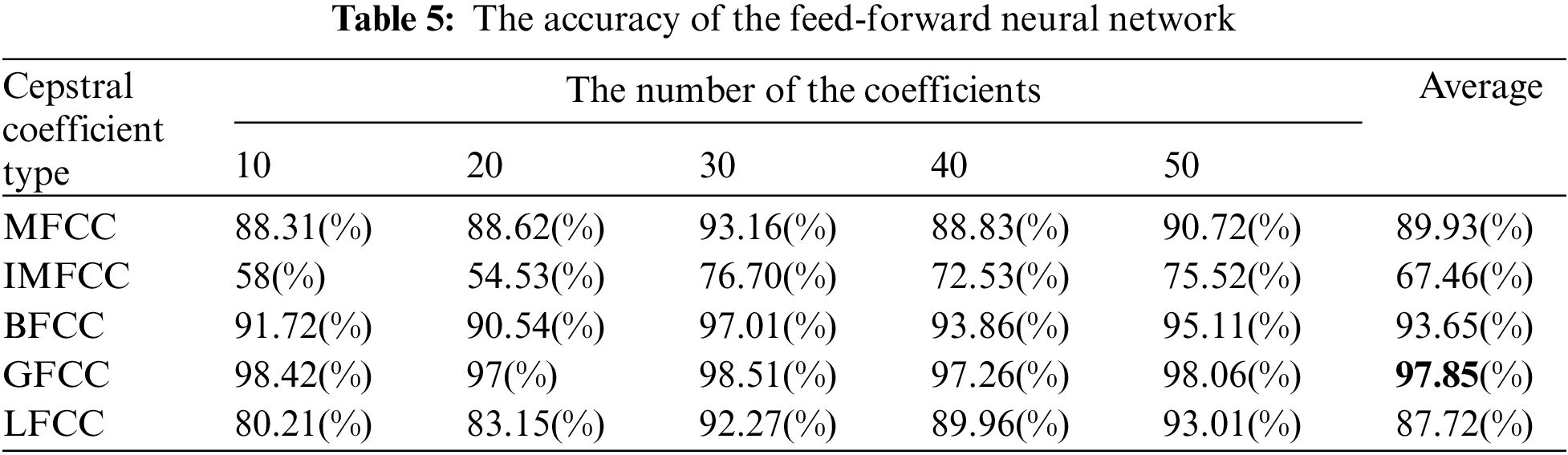
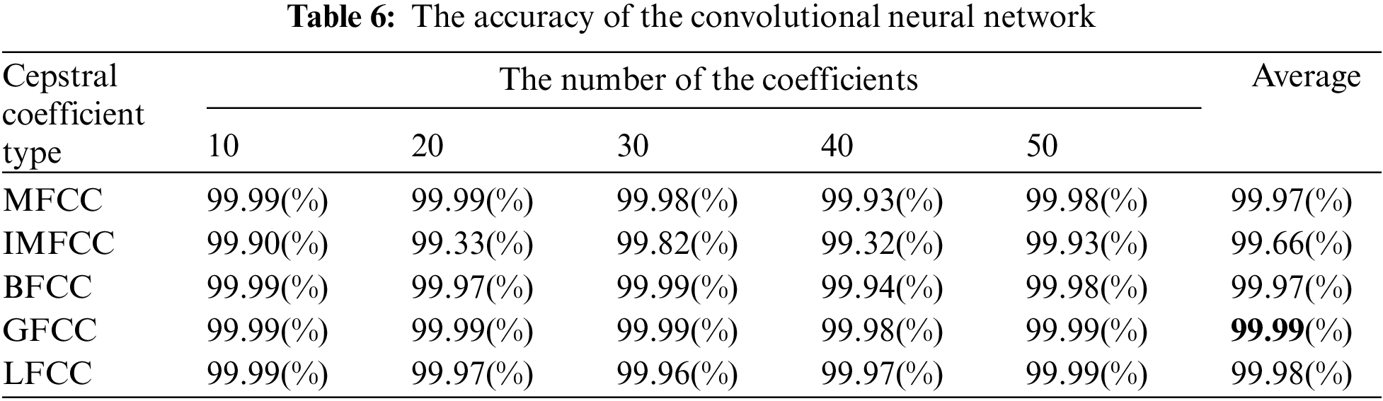
One noteworthy finding in the measurement of the accuracy of device identification is that the GFCC feature consistently produced the highest average accuracy. In detail, when the GFCC features were used as the RF fingerprints, our proposed method produced the highest accuracy of 99.99% for the convolutional neural network model and 97.85% for the feed-forward neural network. We believe that the GFCC feature set contributed significantly to the superior performance of our deep learning model in device identification. The GFCC features had a higher variance of coefficient values compared to the other feature sets, which allowed the model to learn appropriate parameters, such as the weight values of neurons, to distinguish between different types of devices. To confirm this hypothesis, we measured the variance value for each cepstral coefficient feature while varying the number of coefficients. Table 7 summarizes the variance measurement results, which show that the GFCC features had an average variance value of approximately 0.35, while the variances of the other feature sets were much lower. More in detail, the average variance values of GFCC features are approximately 3.80, 3.69, 14.6, and 1.73 times higher than those of MFCC, IMFCC, BFCC, and LFCC, respectively. This observation was further supported by the heatmap examples of the different feature sets, as shown in Figs. 11–15. These heatmaps revealed that the coefficient values in the GFCC example were better differentiated than those in the other examples, as evidenced by the distinct color patterns in the heatmap cells. These results suggest that the higher variance of GFCC features contributed to their effectiveness in discriminating between different devices.

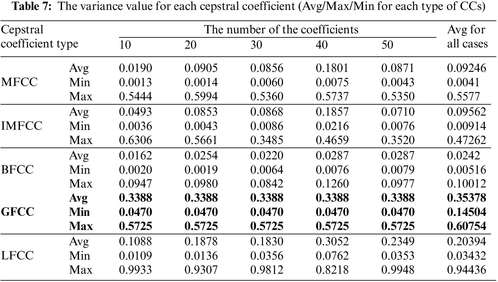
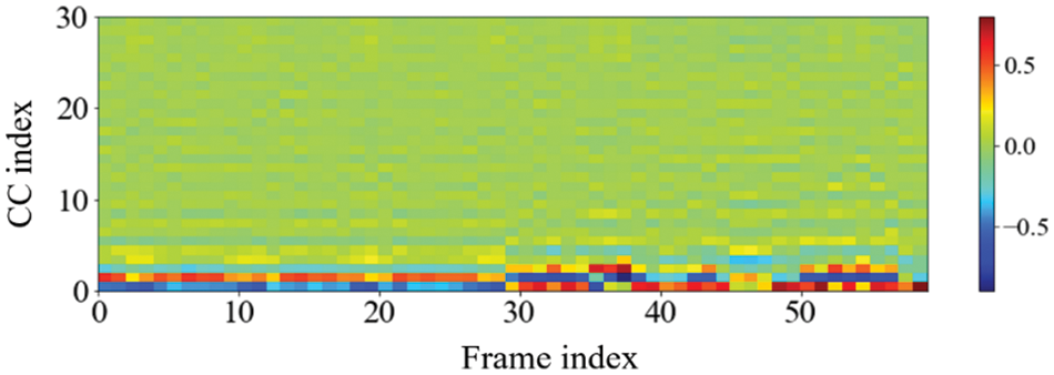
Figure 11: The example of the heatmap of the MFCC

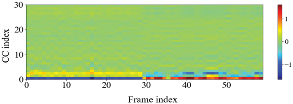
Figure 12: The example of the heatmap of the IMFCC

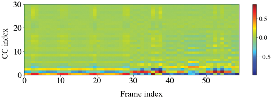
Figure 13: The example of the heatmap of the BFCC

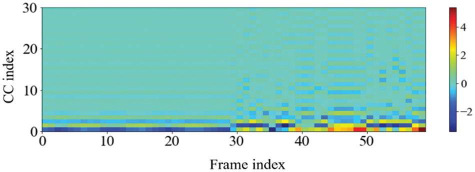
Figure 14: The example of the heatmap of GFCC

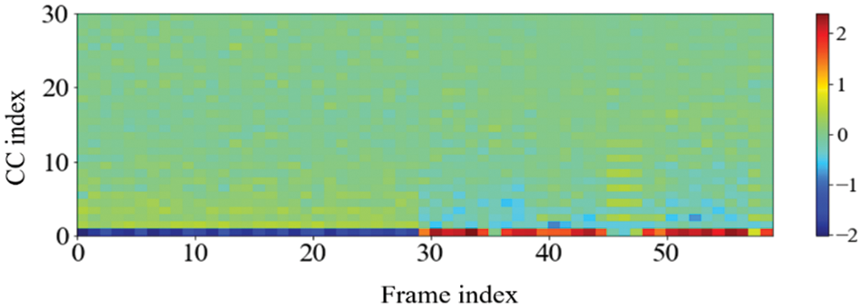
Figure 15: The example of the heatmap of LFCC

Moreover, our experimental results presented in Tables 5 and 6 show that increasing the number of coefficients in the cepstral coefficient features resulted in a consistent improvement in accuracy. We also observed that the accuracy growth patterns of both the convolutional neural network and the feed-forward neural network models were quite similar, despite differences in their architectures and training approaches. We increased the number of coefficients from 10 to 50 in increments of 10 because we observed a noticeable performance improvement when we increased the number of coefficients by 10. The performance improvement plateaued beyond 50 coefficients, with no significant improvement observed, so more evaluation was not performed.

4.3 Performance Comparison with the Other Methods Utilizing Cepstral Coefficients

As described in Section 2, the existing approaches of [7,8] are similar to our proposed method. The methods presented in [7,8] analyze the Mel-Frequency Cepstral Coefficient (MFCC) and Linear Frequency Cepstral Coefficient (LFCC) of radio frequency (RF) signals using a support vector machine (SVM) model or use the quadratic discriminant analysis (QDA) model to analyze MFCC. To compare the performance of our method with these three similar approaches, we implemented them and measured device identification accuracy. As a result shown in Table 8, on average, our best convolutional neural network (CNN) model utilizing the gammatone-Frequency Cepstral Coefficient (GFCC) method achieved approximately 24.5%, 45%, and 26.1% higher accuracy than the SVM-based method utilizing MFCC features, the SVM-based method utilizing LFCC features, and the QDA-based method utilizing MFCC features, respectively.

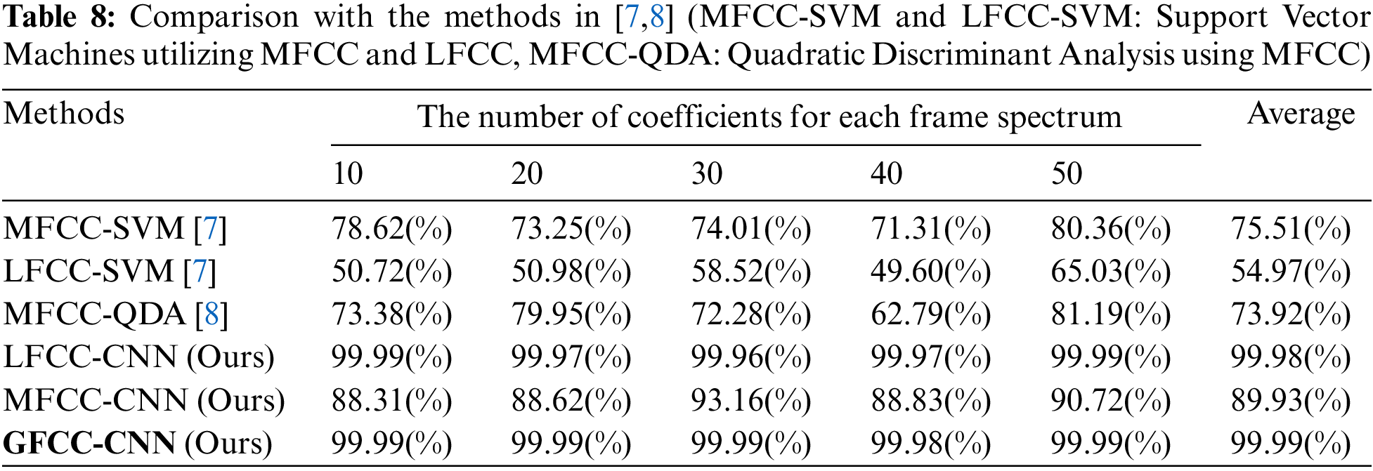
Moreover, both the CNN models utilizing MFCC and LFCC achieved significantly higher accuracies than the SVM model utilizing MFCC, which was the best-performing model among the previous approaches. Notably, even the worst-performing CNN model utilizing MFCC showed an accuracy improvement of 14.4% over the best-performing SVM model utilizing MFCC. These results demonstrate that the CNN model is better suited for processing cepstral coefficient features.

5  Conclusion

We proposed a convolutional neural network-based method for discriminating radio frequency (RF) signals sent by normal RF transmitters equipped with keyfobs for passive keyless entry and start systems. Our method analyzes the RF fingerprint of the given signals using cepstral coefficient features. These features are useful for characterizing the uniqueness of the signal. In an experiment using 20,000 RF signals from 7 different RF transmitters, we found that our method produced the best accuracy when using the Gammatone-Frequency Cepstral Coefficient (GFCC) features as the RF fingerprint. Additionally, we compared the performance of many machine learning-based models. We found that the convolutional neural network outperformed the others, possibly due to its ability to reflect the interrelation information of consecutive overlapped frames extracted from the original signal. In the future, we plan to extend our proposed method by incorporating additional features that can be utilized as RF fingerprints, such as SNR (Signal to Noise Ratio), statistical data like the highest frequency, the lowest frequency, and frequency offset.

Acknowledgement: This work was supported by Institute of Information & communications Technology Planning & Evaluation (IITP) grant funded by the Korea Government (MIST) (No. 2022-0-01022, Development of Collection and Integrated Analysis Methods of Automotive Inter/Intra System Artifacts through Construction of Event-Based Experimental System).

Funding Statement: The authors received no specific funding for this study.

Author Contributions: The authors confirm their contribution to the paper as follows: study conception and design: TaeGuen Kim; data collection & evaluation: Hyeon Park and SeoYeon Kim; draft manuscript preparation: Hyeon Park and Seok Min Ko. All authors reviewed the results and approved the final version of the manuscript.

Availability of Data and Materials: The data that support the findings of this study are available on request from the corresponding author. The data are not publicly available due to privacy or ethical restrictions.

Conflicts of Interest: The authors declare that they have no conflicts of interest to report regarding the present study.

References

1. D. F. Oswald, “Wireless attacks on automotive remote keyless entry systems,” in Proc. Association for Computing Machinery, New York, NY, USA, pp. 43–44, 2016. [Google Scholar]

2. K. Joo, W. Choi and D. H. Lee, “Experimental analyses of RF fingerprint technique for securing keyless entry system in modern cars,” in Proc. NDSS, San Diego, CA, USA, 2020. [Google Scholar]

3. S. Q. Khan, Opening Doors and Stealing Cars: Bluetooth LE Link Layer Relay Attacks. Manchester, United Kingdom: Tech Science Press, 2022. [Online]. Available: https://hardwear.io/netherlands-2022/presentation/bluetooth-LE-link-layer-relay-attacks.pdf [Google Scholar]

4. S. W. Kim and D. W. Park, “Hacking attack and vulnerabilities in vehicle and smart key RF communication,” Journal of the Korea Institute of Information and Communication Engineering, vol. 24, no. 8, pp. 1052–1057, 2020. [Google Scholar]

5. Rolling Pwn Attack. Star-V Lab, 2022. [Online]. Available: https://rollingpwn.github.io/rolling-pwn/ [Google Scholar]

6. K. Joo, W. Choi and D. H. Lee, “Hold the door! fingerprinting your car key to prevent keyless entry car theft,” in Proc. NDSS, San Diego, CA, USA, 2020. [Google Scholar]

7. Y. Diao, Y. Zhang, G. Zhao and M. Khamis, “Drone authentication via acoustic fingerprint,” in Proc. Computer Security Applications Conf., Austin, TX, USA, pp. 658–668, 2022. [Google Scholar]

8. R. Kılıç, N. Kumbasar, E. A. Oral and I. Y. Ozbek, “Drone classification using rf signal based spectral features,” Engineering Science and Technology, an International Journal, vol. 28, no. 101028, pp. 1–10, 2022. [Google Scholar]

9. W. Jin, M. Li, S. Murali and L. Guo, “Harnessing the ambient radio frequency noise for wearable device pairing,” in Proc. Association for Computing Machinery, New York, NY, USA, pp. 1135–1148, 2020. [Google Scholar]

10. J. Gong, X. D. Xu and Y. Lei, “Unsupervised specific emitter identification method using radio-frequency fingerprint embedded InfoGAN,” IEEE Transactions on Information Forensics and Security, vol. 15, pp. 2898–2913, 2020. [Google Scholar]

11. S. Rajendran, Z. Sun, F. Lin and K. Ren, “Injecting reliable radio frequency fingerprints using metasurface for the internet of things,” IEEE Transactions on Information Forensics and Security, vol. 16, pp. 1896–1911, 2021. [Google Scholar]

12. J. Zhang, R. Woods, M. Sandell, M. Valkama, A. Marshall et al., “Radio frequency fingerprint identification for narrowband systems, modelling and classification,” IEEE Transactions on Information Forensics and Security, vol. 16, pp. 3974–3987, 2021. [Google Scholar]

13. T. J. Bihl, K. W. Bauer and M. A. Temple, “Feature selection for RF fingerprinting with multiple discriminant analysis and using Zigbee device emissions,” IEEE Transactions on Information Forensics and Security, vol. 11, no. 8, pp. 1862–1874, 2016. [Google Scholar]

14. L. Peng, J. Zhang, M. Liu and A. Hu, “Deep learning based RF fingerprint identification using differential constellation trace figure,” IEEE Transactions on Vehicular Technology, vol. 69, no. 1, pp. 1091–1095, 2020. [Google Scholar]

15. H. Li, C. Wang, N. Ghose and B. Wang, “Robust deep-learning-based radio fingerprinting with fine-tuning,” in Proc. Association for Computing Machinery, New York, NY, USA, pp. 395–397, 2021. [Google Scholar]

16. H. Maleki, R. Rahaeimehr and M. V. Dijk, “SoK: RFID-based clone detection mechanisms for supply chains,” in Proc. Association for Computing Machinery, New York, NY, USA, pp. 33–41, 2017. [Google Scholar]

17. Z. Zhuang, X. Ji, T. Zhang, J. Zhang, W. Xu et al., “FBSleuth: Fake base station forensics via radio frequency fingerprinting,” in Proc. Association for Computing Machinery, New York, NY, USA, pp. 261–272, 2018. [Google Scholar]

18. S. Wakabayashi, S. Maruyama, T. Mori and S. Goto, “A feasibility study of radio-frequency retroreflector attack,” in Proc. USENIX Association, Berkeley, CA, USA, 2018. [Google Scholar]

19. L. Muda, M. Begam and I. Elamvazuthi, “Voice recognition algorithms using mel frequency cepstral coefficient (MFCC) and dynamic time warping (DTW) techniques,” Journal of Computing, vol. 2, no. 3, pp. 138–143, 2020. [Google Scholar]

20. H. J. Landau, “Sampling, data transmission, and the Nyquist rate,” Proceedings IEEE, vol. 55, no. 10, pp. 1701–1706, 1967. [Google Scholar]

21. A. D. P. Ramirez, J. I. de la Rosa Vargas, R. R. Valdez and B. Aldonso, “A comparative between mel frequency cepstral coefficients (MFCC) and inverse mel frequency cepstral coefficients (IMFCC) features for an automatic bird species recognition system,” in Proc. IEEE Latin American Conf. on Computational Intelligence, Guadalajara, Mexico, pp. 1–4, 2018. [Google Scholar]

22. X. Zhou, D. Garcia-Romero, R. Duraiswami, C. Espy-Wilson and S. Shamma, “Linear versus mel frequency cepstral coefficients for speaker recognition,” in Proc. IEEE Workshop on Automatic Speech Recognition & Understanding, Waikoloa, HI, USA, pp. 559–564, 2011. [Google Scholar]

23. C. Kumar, F. ur Rehman, S. Kumar, A. Mehmood and G. Shabir, “Analysis of MFCC and BFCC in a speaker identification system,” in Proc. Int. Conf. on Computing, Mathematics and Engineering Technologies, Sukkur, Pakistan, pp. 1–5, 2018. [Google Scholar]

24. J. Qi, D. Wang, Y. Jiang and R. Liu, “Auditory features based on gammatone filters for robust speech recognition,” in Proc. IEEE Int. Symp. on Circuits and Systems, Beijing, China, pp. 305–308, 2013. [Google Scholar]