Explainable Artificial Intelligence-Based Model Drift Detection Applicable to Unsupervised Environments

1  Introduction

1.1 Motivation

The rapid pace of data growth has led to developing new attack methods that are rapidly evolving. In response, the security industry has recognized the need to incorporate machine learning (ML) techniques into security systems and is researching to detect new, previously unknown attacks. With the growing interest in ML, ML operations (MLOps) have emerged for efficient management. Before MLOps, a culture and methodology called development and operations (DevOps) was combined to operate applications efficiently. Later, MLOps emerged to operate artificial intelligence (AI) and ML efficiently. These MLOps play a critical role in the social atmosphere, which requires smooth system operation in an environment where data exchange and change coexist. Models introduced into the system are maintained through MLOps to increase model sustainability in the post-deployment environment. Model management is essential for ML models, especially in the networking field, to withstand the massive amount of data generated in a short period. In network security, changes in new data or the discovery periods of a model can be interpreted as the occurrence of new attacks and the deterioration of the detection performance of existing models, a severe problem that negates the reason for the model. Therefore, as a follow-up, such measures as data reorganization and model retraining can be taken to increase model sustainability.

For efficient system operation and effective model management, monitoring the health of models in real time is crucial. Drift manifests in various forms, including model, data, and concept drift, with data drift being the most prevalent. This type of drift can lead to significant issues, such as rendering existing models obsolete and necessitating comprehensive system reconfiguration. Swiftly identifying drift signals within management and oversight processes is essential to ensure a sustainable system operation and prompt response. Typically, drift can be inferred when metrics, such as accuracy or error, deviate from the previous performance by more than a certain threshold. However, detecting performance drift necessitates access to correct answers for model predictions, which can be time-consuming and costly in real-world settings. Existing drift detection methods (DDMs) predominantly cater to supervised environments where performance changes are informative but rely on ground truth labels. These approaches are constrained by their inability to differentiate between distinct drift types, such as data and concept drift.

No matter how good a detection method is, the most crucial aspect is whether it can be applied in a real-world environment. Monitoring is essential to detect real-world drift. Monitoring the currently running model in real time is essential to detect drift and react quickly with corrective actions. Therefore, supervised environments that are far from real time are inappropriate. Effective management and supervision require DDMs that are less dependent on answer sheets and are applicable to unsupervised environments.

1.2 Contribution

The proposed method in this paper seeks to address the limitations of existing model drift detection techniques, offering several vital contributions, as outlined below. First, the approach is designed for application in unsupervised environments, which is critical for practical implementation within the industry. The proposed technique adopts a well-suited measurement approach for unsupervised settings by employing a density-based distance method. Second, the method is model-agnostic, accessible, and reliable. Leveraging explainable AI (XAI) technology ensures the explainability of model prediction outcomes through various plots and explanations, an aspect absent in the current methods. Last, the numerical representation of drift signals delivers intuitive drift suspicion results for individual data points, enabling a detailed analysis through the examination of specific data. This paper aims to demonstrate a novel possibility for drift detection by expressing the change in the influence of each feature as a distance-based score while measuring the extent of statistical change using a predetermined threshold.

2  Related Work

2.1 Importance of Model Management and Drift

Deploying an ML model creates the best model for the environment during design. However, it is difficult to maintain the same performance even after the model is deployed if it is designed according to the system environment and the designer’s intentions. Therefore, several factors must be considered for smooth operation by management/supervision of the deployed ML model, as presented in Fig. 1 [1].

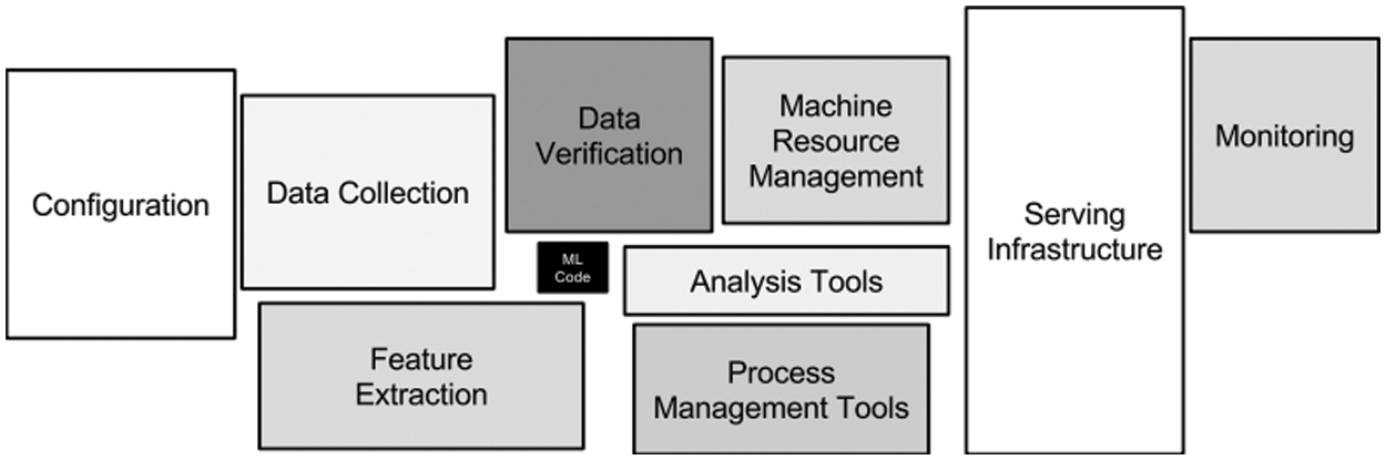
Figure 1: Machine learning system elements

In recent years, as ML has become more widespread, the concept of MLOps has emerged as one of the most promising trends [2]. Moreover, MLOps implements five functions that integrate the development and production phases of ML: (1) data collection/transfer, (2) data transformation, (3) continuous ML retraining, (4) continuous ML redistribution, and (5) production/presentation output for end users. The goal of MLOps is to support the automation, integration, and monitoring of these phases [3]. After a model is deployed, the environment may change; in particular, changes in data statistics, prediction labels, and attributes may cause drift, reducing the persistence of the model. In this paper, we focus on efficient model management methods that monitor the progress of (2) through (4) of the five features to contribute to the mentioned model drift detection.

Focusing on model drift during monitoring is vital because it signals environmental changes caused by data drift and the need for retraining. Failure to recognize changes in the model can lead to severe problems, such as false positives and malfunctions. For example, industrial control systems undergo continuous digital transformation and maintenance with real-time monitoring. Rapid malfunction and drift detection can eventually lead to a healthy system lasting longer than the expected lifespan [4].

Security systems constantly change, and ML models are introduced in earnest to detect new and unknown malicious behavior. However, it is impossible to detect all myriad types of malicious data in the vast data environment. Therefore, models are often built by introducing detection techniques specialized for specific attacks, such as malicious data and spam [5]. However, there are limits to how well malware detection models can keep up with evolving attack techniques. Eventually, drift occurs when the model fails to adapt to changing data, directly influencing model performance, or when new attacks emerge that differ from the original data. Drift in security systems can have dire consequences when considering emergency services, so drift mitigation is essential to eliminate adverse effects.

While the goal is to detect drift quickly and accurately to manage the life cycle of a model, drift is caused by many diverse types of changes. It is more sensitive in network systems where vast data are generated quickly. Therefore, efficient, lightweight, scalable drift detection techniques are needed to be applicable in such network systems [6].

2.2 Different Approaches to Detecting Model Drift

Fig. 2 depicts a typical example of drift detection [7], which detects drift signals by comparing predeployment data with new post-deployment data.

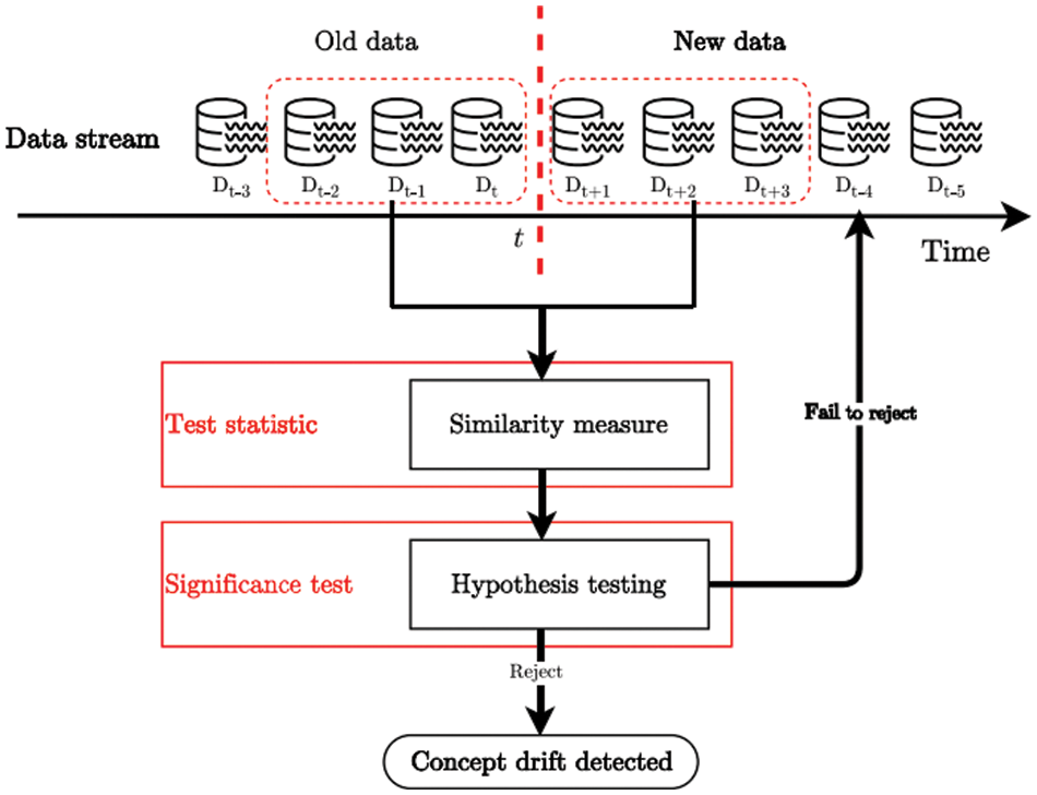
Figure 2: Common examples of drift detection. Adapted with permission from reference [7]
Adapted with permission from Ref. [7]

2.2.1 Methods for Detecting Model Drift

The DDMs can be broadly categorized into supervised and unsupervised environments. Supervised environments detect drift when the sample and comparison data are labeled. Drift detection is essential in environments that deal with numerous data, such as weather, network logs, and alerts from industrial systems. Therefore, a drift detector must be introduced that can be applied in an unsupervised rather than a supervised environment to detect whether the target data have drifted, although labels may exist in the learning drift or inferring statistics processes [8].

Detection methods in unsupervised environments depend on data availability, as illustrated in Fig. 2, and can be categorized into batch methods that set the batch size within limited data and online methods that consider all incoming data at a specific time. Even within batch methods, methods are further divided into those using full batches [9,10] and those using partial batches [11]. Online methods can again be divided into fixed reference methods based on reference windows and sliding reference methods for data with fewer labels [12,13]. In both methods, similarities are compared after the data have been accessed.

Similarity comparison is a step that directly detects the drift between the reference and comparison data. There are methods to detect similarity based on performance changes, such as accuracy, recall, sensitivity, and error rates. A typical example is the DDM, a performance-based drift detector [8]. The DDM assumes that a drift signal appears when the change in a metric exceeds a significance level. The DDM has since evolved into other performance-based detection methods [14,15]. As mentioned, these methods can be measured in the presence of labels in a supervised environment. However, they have the disadvantage of being highly dependent on labels.

Several nonperformance-based detection methods have been developed to compare similarities using statistical measures. These approaches measure the distance from the target of comparison and employ it as a drift detection metric [16]. Techniques, such as distance-based measures, Kolmogorov–Smirnov tests, clustering similarity, and margin density, have been used for drift tracking as an alternative to traditional statistics. A significant advantage of these statistical DDMs is their ability to operate effectively without labels. One method proposed for monitoring distribution changes in a sliding window fashion signals a drift when the number of identified outliers surpasses a specified threshold [17]. Additionally, new DDMs leverage the density of posterior probabilities in semi-supervised environments, making them suitable for streaming environments with limited data labels [18].

2.2.2 Explainable Artificial Intelligence-Based Methods for Detecting Model Drift

The exceptional performance of ML methods, combined with technological advances, has led to widespread adoption across numerous domains. However, these models inherently present a trade-off between performance and transparency. Despite achieving high-performance metrics, how these models form predictions and judgments remains unclear, often leading to their classification as black-box systems [19]. Consequently, stakeholders increasingly demand model transparency. In response to this need, the US Defense Advanced Research Projects Agency has proposed XAI [20], an approach aimed at developing interpretable models while maintaining the performance of existing models, garnering considerable interest within the field.

These XAI techniques can be categorized into interpretable models that provide explanations on their own and techniques that employ external explanatory approaches. External techniques provide additional value by providing statistics, visualizations, examples, and other methods to explain the basis for predictions and judgments. The interpretability of a model is essential information in the process of tracking model drift. Analyzing its causes through interpretability and drift detection has helped overcome the limitation of not having immediate feedback on the model output in real-world scenarios [21]. In addition to traditional drift tracking methods, research on drift detection provides evidence for drift [22]. This study revealed that drift detection and the rationale could be explained by tracking features that cause significant changes in the distance between distributions.

Lundberg et al. proposed Shapley additive explanations (SHAP) based on the Shapley value for model explanatory power [23]. The SHAP value measures the influence (contribution) of each feature in the data in explaining model predictions. Based on this, we present a variety of plots to provide explanations that can be interpreted locally and globally. A growing body of research combines SHAP with AI models to interpret complex internal structures with applications in health care, security, and other fields.

Lundberg et al. proposed a variety of uses for SHAP [24]. Fig. 3 presents an example of post-deployment monitoring of a model using SHAP values. Fig. 3b depicts an example of the possibility of detecting errors through the change in SHAP when the data are partially relabeled. Fig. 3c illustrates the possibility of detecting specific functional errors due to problems with the system’s internal measurement methods. We compared Figs. 3a and 3d to illustrate the potential use of drift detection. The graph in Fig. 3a presents the overall loss of model predictions commonly used for drift detection. This graph naturally displays the inevitable increase in loss with testing data, but from the perspective of drift detection, it is difficult to determine the onset and progression of drift from this graph alone. Fig. 3d displays the SHAP value for the loss function of the model. We argue that if a gradual drift occurs, the drift can be recognized by the change in SHAP loss, as indicated in the graph. Similarly, a study has shown that SHAP values can detect drift in individual features through changes in sensitive features [25]. In this study, changes in individual features over time as drift occurs were observed through changes in SHAP values, revealing that drift can be recognized in advance through intuitive changes in individual features that begin to exhibit different distributions as drift occurs.

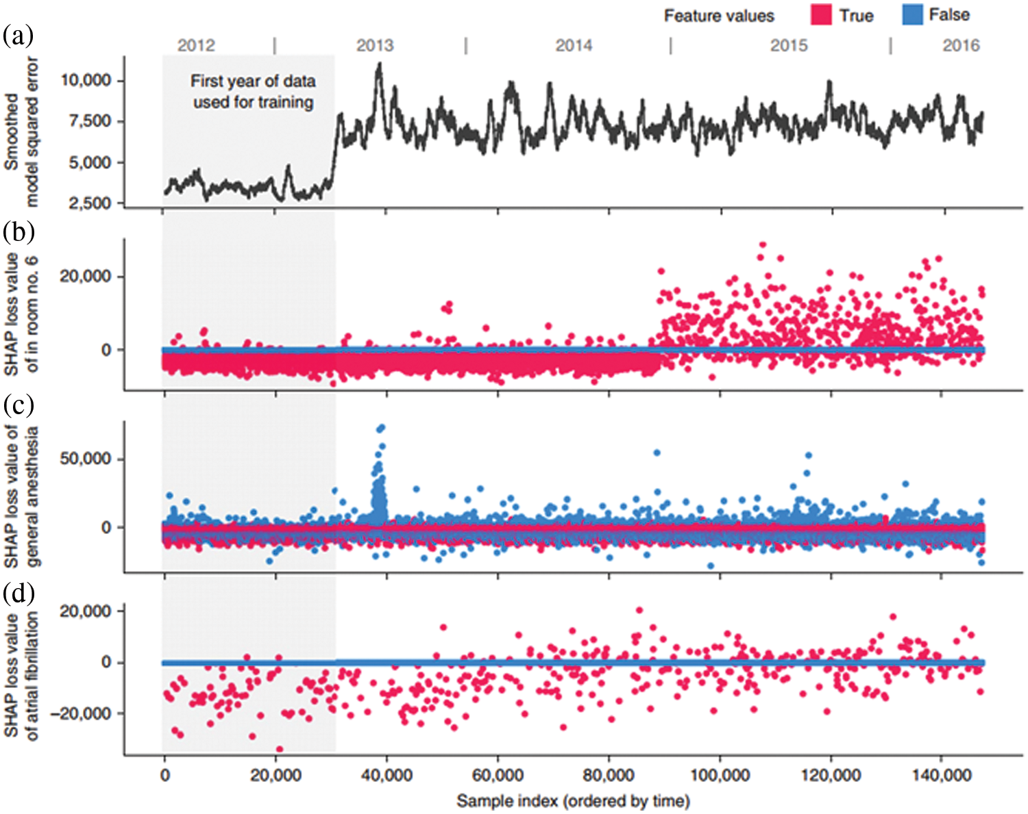
Figure 3: Example of monitoring plots. Adapted with permission from reference [24]
Adapted with permission from Ref. [24]

Previous research has found that drift detection signals the need for model management, an essential task that should be performed concurrently with model deployment. In particular, the security field requires monitoring for drift detection to create systems that respond in real time to new attacks without collapsing. In this paper, we propose a multivariate data-tailored drift signal extraction method and a detection method that can be introduced to unsupervised environments by reducing the reliance on labels.

3  Proposed Method

Monitoring for drift detection is crucial in managing constructed AI models, as it facilitates the identification of issues within the model and data. However, regarding data types for drift detection, numerous studies have concentrated on supervised environments and encountered limitations, such as losing significant attributes due to dimensionality reduction while measuring the similarity to reference data. This paper introduces a method that leverages SHAP values, representing the influence of features in the AI prediction process within XAI. This approach prevents substantial data loss and offers a drift detection technique applicable to unsupervised environments. Fig. 4 outlines the process of the proposed method.

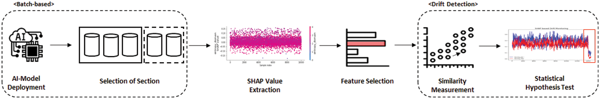
Figure 4: Overall structure of the proposed method

3.1 Data Generation Including Drift

Selecting a data configuration is the first step in tracking data of a different nature than before the model is deployed. As presented in Fig. 2, there are old and new data for drift estimation. The old data are the data before the deployment and the reference data for drift detection. New data are data after deployment, and drift is detected in these data. Therefore, in selecting data for drift detection, the reference data should consist of representative data representing the currently deployed model well, such as training data. Data subject to drift detection can be the testing or new data generated after deployment.

3.2 Selecting Important Features

Features are crucial elements representing model characteristics to comprehend and learn from data. Typically, numerous features are constructed to maintain a wide range of possibilities among the data characteristics to predict the label. However, among the vast array of features, only a few features play a pivotal role in determining the label. Consequently, any alteration in these critical features affects the label, model, and other aspects.

In this study, we aim to select essential features from the extensive pool to identify a limited number of critical factors and detect drift through changes in these features. We employed SHAP as a tool for selecting these critical features, which generates descriptors to represent the constructed model and extracts SHAP values by estimating the model.

Moreover, SHAP was implemented as a Python library to provide a variety of plots. Summary and monitoring plots were used to screen and determine the most influential features based on the analyst’s expert opinion. Fig. 5 is a representative example of a summary plot, which visualizes the influence and magnitude of all features in a label. Influence considers the positive and negative contributions of the features to the label, and they are listed in order of increasing influence. Distributions to the right of the center are positive for the label, and those to the left are negative. The color of each point represents the actual feature value, and the magnitude of the value can be interpreted as the influence.

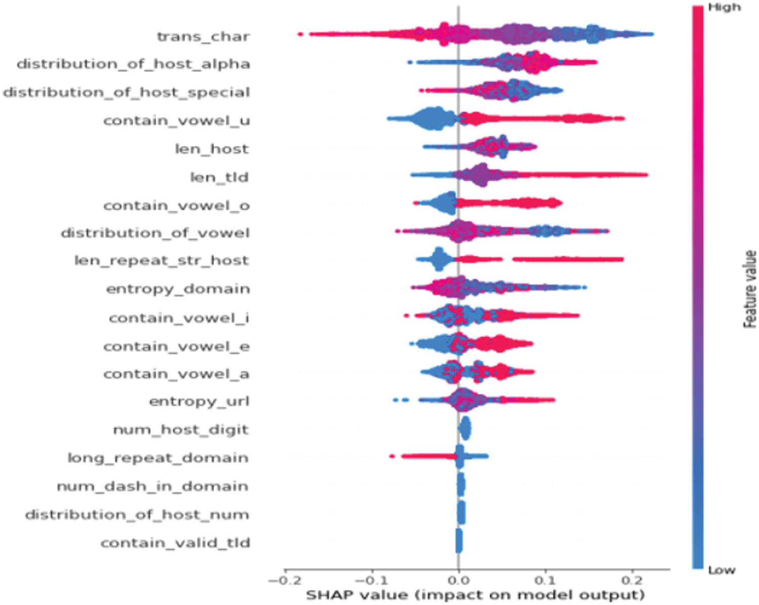
Figure 5: Example of summary plots

The top features are selected as critical by judging the degree to which their influence distribution is evident. Because the summary plot takes the absolute values of the positive and negative influences from an overall perspective and assigns a differential based on the overall sum, it is not always clear that the top features provide clear direction. Therefore, analysts use monitoring plots to determine which features are clear. Fig. 6 plots the relationship between the actual and SHAP values of a feature in index order. In the monitoring plot above, the actual values are not distributed in a specific range and do not have a clear area of influence. These features appear as top features in the summary plot but do not appear in a specific section and have a random distribution. The process of selecting critical features aims to track down and remove these features from the list and identify those features that demonstrate clear influence and interpretability as crucial, such as the monitoring plot below.

Figure 6: Example of selecting vital features by monitoring plots

3.3 Similarity Measurement

The subsequent step, which is crucial for drift detection, involves measuring similarity. Drift fundamentally involves assessing statistics that differ from the original data; thus, most DDMs measure similarity by comparing the statistics of the reference and comparison data based on a predetermined threshold. In unsupervised environments, distance is commonly measured to determine similarity. For multivariate data, dimensionality reduction is required for distance calculation, clustering, visualization, and other purposes. However, a caveat in this process is the potential loss of meaningful information during the dimensionality reduction procedure. This study proposes a similarity measurement method employing SHAP values to address these limitations, as outlined in Table 1.

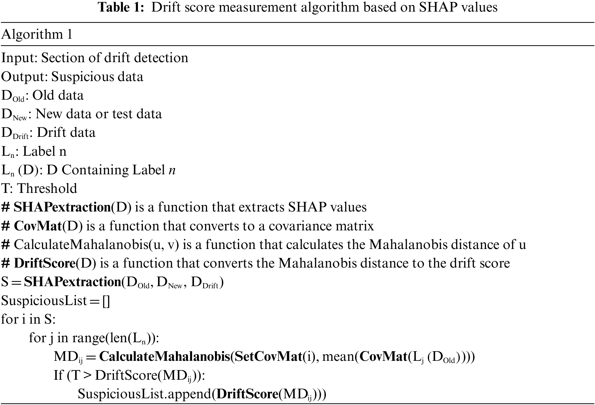
The SHAP values function as a tool for selecting key features and as a substitute for actual values in distance measurements. Using SHAP values instead of original values presents several advantages. First, SHAP values serve as a numerical representation of the influence of each feature, enabling them to be weighted according to their importance and emphasized during the comparison process. Second, all data and features can be compared using the same standard unit. While raw values exhibit distinct units, scales, and ranges, SHAP values allow comparisons within the same space, overcoming these limitations. Last, SHAP values describe the model decision-making process; thus, each step is accompanied by an explanation, such as the rationale behind the decision, enhancing the credibility of the process.

After the data transformation, we measured the distance using the Mahalanobis distance metric. The Mahalanobis distance allows for a more meaningful interpretation than the Euclidean distance. The Mahalanobis distance is ideal for multivariate data environments because it considers probability distributions. Specifically, while the Euclidean distance is a simple distance calculation, the Mahalanobis distance is a density-based distance measure that considers the associations in the data. The formula for the Mahalanobis distance is calculated as follows:

d(u, v)=(u−v)∑−1(u−v)T.(1)

1

In the expression, u is each data point, and v is the mean of the data. The Mahalanobis distance method is a probability distribution-based calculation that requires data to be transformed into a covariance matrix to measure the distance. After converting the data into a covariance matrix that considers the correlation between the variables, the Mahalanobis distance is measured.

The Mahalanobis distance measure is combined with the drift measure and expressed as a p-value to derive a statistically significant interpretation. The Mahalanobis distance follows a chi-square distribution, and the goodness-of-fit test compared to the population during the chi-square test is essentially similar to drift detection.

3.4 Statistical Hypothesis Test

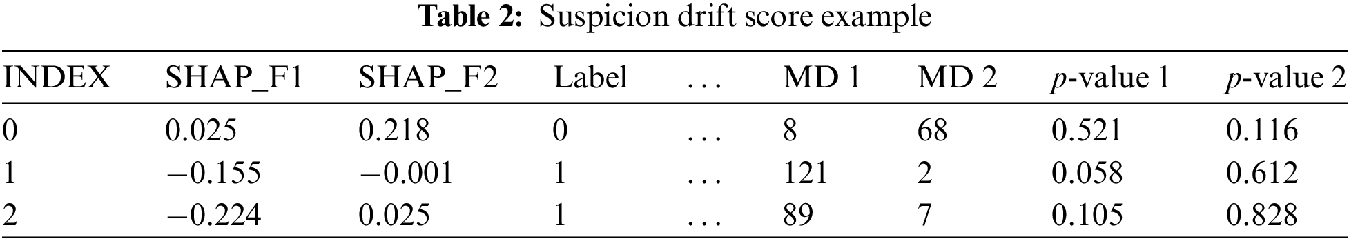
The drift score, derived from the SHAP of new data relative to the predeployment data, represents a probabilistic interpretation of the Mahalanobis distance value. Data points with p-values below a specific threshold are typically classified as statistically deviant in statistical comparisons. Consequently, by applying the drift score threshold, values identified as statistically deviant are categorized as suspected drift data.

Table 2 is an example of measuring the drift score for individual data. The values SHAP_F1 through SHAP_Fn represent the SHAP values of the features to obtain the Mahalanobis distance. Moreover, MD 1 and MD 2 correspond to the distance of the data from each label in the data before the distribution, and p-values 1 and 2 correspond to the final drift score as a probability value for the distance. The MD value means the data point is farther from the corresponding label. In turn, p-values can be interpreted as moving away from the threshold. A p-value below the threshold indicates a deviation from the existing distribution, which can be interpreted as drift. As an example of this interpretation, suppose the threshold is 0.1, and p-values 1 and 2 are below 0.1. Any p-value that falls below the threshold can be viewed as a drift, which can be considered an instance of drift away from the current statistics.

Because drift scores are measured as the distance of individual data points from the existing labels, even in unsupervised environments with limited labeling, one can classify suspected drift data based on drift scores alone. These classified suspected drift data can be accumulated in a database to track the actual drift start point. Fig. 7 illustrates the result of accumulating drift scores from the analyzed data during monitoring. Analysts can infer that drift has occurred when the curvature of the graph differs from the traditional statistics, as presented in the figure.

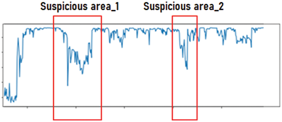
Figure 7: Example of measuring the drift score

4  Experiment

The experiments in this section were designed to validate the proposed method. We focused on detecting domain generation algorithm (DGA) attacks, one of the types of network attack detection. The dataset consists of previously trained DGA data and scenarios where the DGA of various types occurred after deployment. This experiment aims to validate whether the deployed model can detect drift when a DGA of a different nature from the original distribution occurs over time. In a real-world environment, the post-deployment data have limited labels, but because this experiment aims to validate the proposed method, we constructed labeled data for cross-validation. Therefore, the result evaluates whether the model can detect drift occurrence.

4.1 Dataset

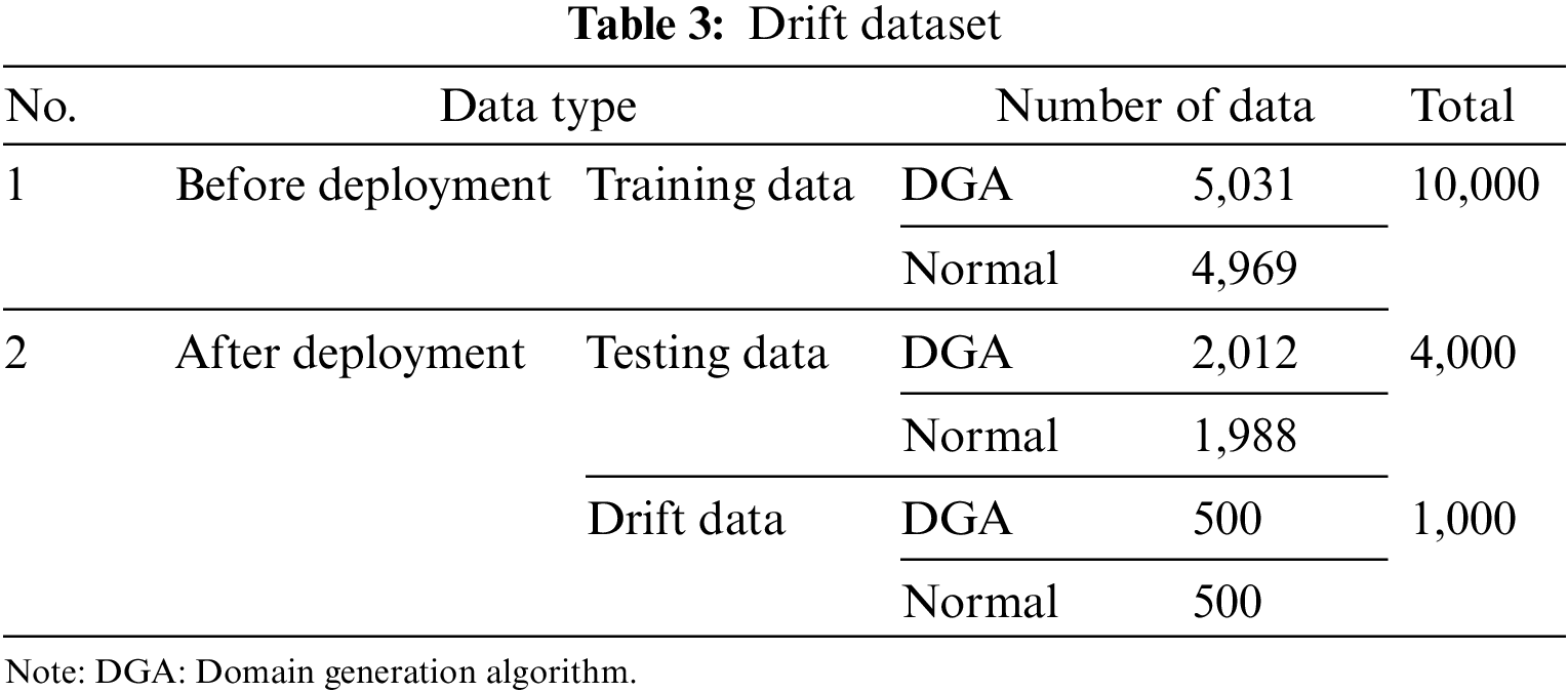
The experiment is to validate drift detection; thus, we require data of the same nature as the existing distribution and data of a new nature. The dataset consists of a DGA dataset provided by NetLab and a general domain dataset provided by Alexa, as presented in Table 3. The dataset consists of conditions under which drift can occur in the DGA detection model.

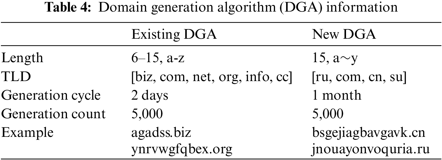
After deployment, we added a new DGA of a new nature to create an environment where drift occurs. Information about the previously trained and new DGAs is provided in Table 4. When comparing the old and new DGAs, drift will likely occur due to the different lengths and randomized alphabets, which degrade the performance of the old model.

4.2 Preparation Process for Drift Detection

We constructed a model with the previous training data to create a drift detection environment and extracted SHAP values as descriptors. Then, instead of using all the features for drift detection, we used SHAP plots to select critical features.

4.2.1 Model Creation

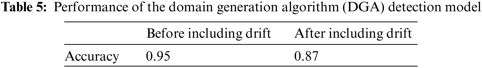
The DGA detection model is generated from the training data before deployment. This experiment aims to validate whether the proposed method can detect drift. The validity of the generated model and dataset is also a factor that must be validated during the process. The generated dataset contains a different data type than the trained data. Therefore, for the generated model and dataset to be valid, the data after deployment must display a degradation in performance compared to the results predicted by the model. It is usual for models to perform poorly on new data types because they are specialized for the existing types. Although the proposed method is a DDM applicable to unsupervised environments, we validated the models and datasets by constructing labeled data for validation. The resulting performance changes in the generated models are presented in Table 5.

4.2.2 Selection of Important Features Based on SHAP

The proposed method uses SHAP values from existing data to overcome the limitations of existing DDMs. We extracted the SHAP values through a descriptor that mimics the generative model, and based on these values, we used the summary and monitoring plots among the various plots provided by the SHAP values. The first step in selecting vital features is to employ the summary plots to obtain a list of high-influence features, as illustrated in Fig. 8. The order of the summary plots is determined by the sum of the absolute values of the SHAP values to obtain a high-influence list.

Figure 8: List of high-influence features

While the summary plot provides an overview of the overall influence, the distribution of SHAP values differs for each feature. Therefore, the next step is to use the monitoring plot. The monitoring plot helps characterize each feature by displaying the distribution of the SHAP values in detail. In Figs. 9a and 9b, the results of the monitoring plots are provided for “trans_char” and “distribution_of_vowel,” where (a) displays the difference between positive and negative influences based on the actual values. Features with clear boundaries of influence and interpretation, such as in Fig. 9a, are added to the list of critical features. In contrast, features with unclear boundaries, such as in Fig. 9b, are removed from the list because their interpretation is unclear. Following the above process, 10 vital features were selected: “trans_char,” “distribution_of_host_special,” “len_host,” “len_tld,” “len_repeat_str_host,” “contain_vowel_u,” “contain_vowel_o,” “contain_vowel_a,” “contain_vowel_e,” and “contain_vowel_i.”

Figure 9: Monitoring plot results of the exclusion target

4.2.3 Drift Score Extraction

The drift score is determined by the Mahalanobis distance between the two labels in the data before the distribution. We must first perform a covariance matrix of the SHAP values and measure the Mahalanobis distance between the DGA and dataset corresponding to the typical region. This measure is a distance, so a higher value means a deviation from traditional statistics. However, the distribution of the values is unclear, and a probability transformation is made to facilitate analysis.

Fig. 10 presents the distribution of drift scores after data allocation for an overarching analysis of the results. Each distribution groups the labels predicted by the model, excluding drift data, enabling the observation of trends in drift scores. In the graph, 0 represents the drift score for normal data before allocation, while 1 signifies the drift score for DGA. The first distribution pertains to data with predictions classified as normal. Although a wide range of distributions exists for normal, most of the p-values for the DGA are below 0.1. The second distribution corresponds to results predicted for the DGA, which similarly exhibits a low p-value for normal. These findings indicate that a low p-value emerges when the drift scores of the proposed method possess distinct statistics compared to the measured labels. Consequently, the low p-value for the normal and DGA data can be interpreted as data exhibiting novel statistical characteristics.

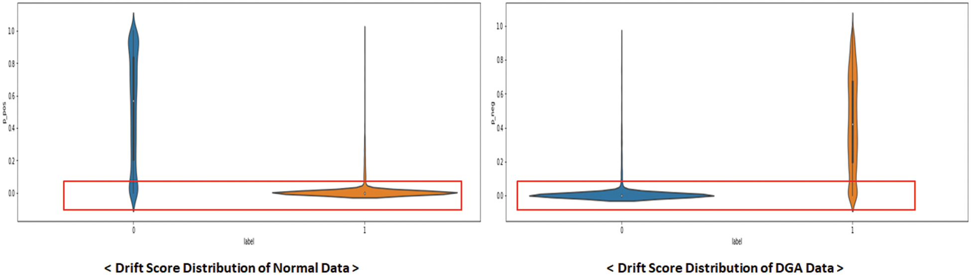
Figure 10: Drift score distribution for all data

Table 6 presents some of the results. In the first and second cases, drift occurs in the data, but the distances and probabilities for both DGA and normal data exceed the threshold. These cases are considered to have drift because the existing labels deviate from the statistics. For this experiment, we assumed that drift is suspected if the p-value is 0.1 or less.

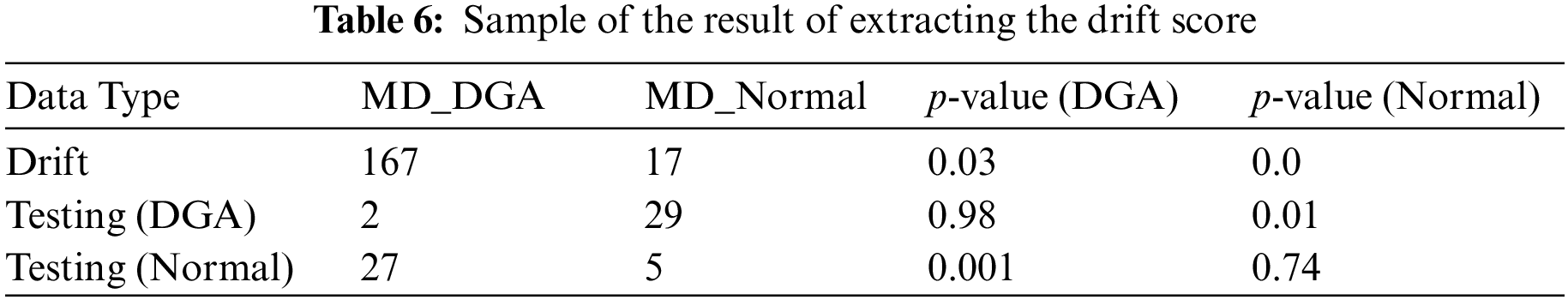
4.2.4 Statistical Drift Tracking and Analysis Results for Extracting the Drift Score

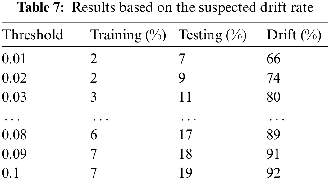
After extracting the drift score, one can check whether the data drifts based on the set threshold. It is crucial to determine the optimal value for the threshold, as the strength of the threshold determines the detection rate of drift in the analyzed data. Table 7 lists the percentage of suspected drift in the data based on the threshold. Drift is when the drift scores of the normal and DGA data in the predeployment data are lower than the threshold. Training and testing refer to the percentage of suspected drift in the normal and DGA data combined, whereas drift refers to the percentage of suspected nondrift in the new DGA data. The lower the percentage of suspected drift in the nondrift testing data and the higher the percentage of suspected drift in the drift data, the better the results. The results reveal that a lower threshold results in a lower percentage of suspected drift in the actual drift data. Therefore, setting the optimal threshold to track the occurrence of drift is of utmost importance.

The proposed method allows setting a threshold to distinguish between individual data and data suspected of drift. It can also be used to track the overall occurrence of drift by inferring the occurrence of drift from the moving average line of drift scores. Fig. 11 depicts the moving average line for drift scores, and Fig. 11a displays the moving average line for drift scores for data that the model predicted would be in the normal region of the overall data. Conversely, Fig. 11b presents the moving average line for the data predicted to be in the DGA region. All figures have in common that the average moving line changes as it moves from the training to the testing data. This change is natural because the initial training and testing data statistics are subtly different. However, if the average moving line drops after the testing data, the data have different properties than the original data, and the analyst must determine whether drift has occurred. Only by categorizing the data according to the labels predicted by the model and comparing the drift scores can the model detect data of a noticeably different nature. Visualizing the classification by the mentioned thresholds can be used as a helpful indicator for analysts to determine drift.

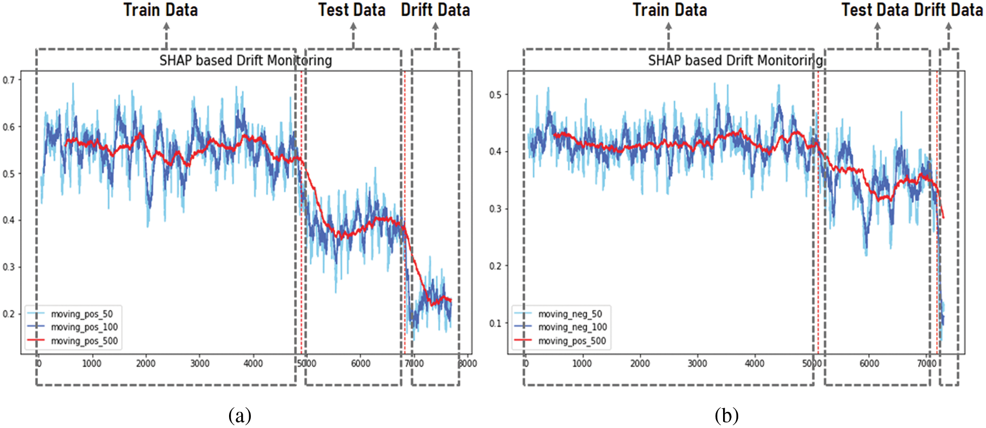
Figure 11: Average moving line results for the drift score

The first observation method we implemented in this experiment was to measure the drift suspicion rate as a function of the threshold, and the results revealed that the drift-induced data have a high drift suspicion rate as a function of the appropriate threshold. We also detected the second observation method, the moving average line of the drift scores for each group of labels. Similarly, a sharp drop in the moving average line was observed at the beginning of the drift-inducing data. Thus, the experiments demonstrate the validity of the proposed method as an approach to detect drift-induced data that are presumed to be new labels.

5  Discussion

The DDM we propose is an innovative approach to overcome the limitations of existing detection methods and environments for model drift detection. The experimental results demonstrate that this approach can quickly detect drifted data.

The proposed approach offers several advantages for its application in model drift detection. First, it delivers an intuitive numerical representation of drift signals, assigning a drift score to each data point. By setting arbitrary thresholds for the drift score, the approach yields easily interpretable results based on well-defined criteria. Second, the method is model agnostic, making it applicable across models. Moreover, SHAP facilitates the calculation of individual feature influences on the predicted outcomes, enhancing the understanding of the model decision-making process and fostering increased confidence. Last, the approach accommodates conditions suitable for unsupervised environments, a crucial requirement for conventional drift detection. As a numerically conditioned detection method rather than a label-based one, it exhibits less dependency on labels.

While the proposed method is promising for application to various drift detection environments, the limitations must be addressed in future research. First, comparison targets under different conditions are needed in the experimental stage for drift detection. The validity of the proposed method must be further verified through the results of comparison targets in various environments. In the future, we plan to verify the validity of drift detection in other scenarios by applying the proposed method based on cases using AI models in other security areas besides DGA detection scenarios. In addition, we plan to introduce a comparative analysis method that considers both the explainability and ability to detect drift data combined with XAI to clarify the validity of the comparison method with other scenarios. Second, the speed of the drift score calculation must be improved, which is a factor in determining the presence of drift. The most significant problem with drift scores is that they are time-consuming to calculate when extracting the SHAP values on which they are based, which requires a fundamental solution that has not been addressed despite efforts to extract them quickly, such as fastSHAP and GPUTreeSHAP. The final limitation is that, although the proposed method helps detect different data types in existing environments, it requires an additional step of aggregating drift from individual data to determine when model drift occurs.

6  Conclusion

In the rapidly evolving cyber landscape, effectively combating various threats necessitates the prompt and accurate detection of drift signals in models to prolong the lifetime of the deployed models. Although existing studies on drift detection primarily focus on supervised environments, the reliability of the metrics determining drift remains uncertain. During data preprocessing for drift detection, labels can be applied to predeployment data; however, labeling operations are limited for subsequent data. Consequently, drift signal detection methods suitable for unsupervised environments where labeling operations have minimal influence are necessary to facilitate real-world applications.

This paper introduces a method for drift detection that is independent of labels and considers explanatory power. The framework of the proposed method aims to identify drift signals by extracting a drift score, a statistical metric to classify and assess whether data exhibit drift during the monitoring process. We extracted the SHAP values to obtain the drift score for each data point. This approach offers significant advantages by overcoming existing limitations and leveraging various SHAP features with high descriptive power for a fair comparison across all features. Subsequently, we calculated the Mahalanobis distance-based drift score and evaluated drift in individual data points based on a predefined threshold.

To assess the effectiveness of the proposed method in augmenting the explanatory power of existing data and drift detection techniques, we conducted experiments within a DGA detection context. We designed the data scenarios to incorporate new DGAs exhibiting distinct characteristics compared to those of previously trained DGAs and applied the proposed approach to extract drift scores for each data point. Thus, the drift scores of the new DGAs were higher compared to the actual labels of the data classified as suspected drift data. The experimental results reveal that the proposed method can detect suspected drift data with new labels. Additionally, as the proposed method derives drift scores using SHAP values, it offers explainability throughout all stages of assessment and implementation, bolstering confidence in the approach. This study applies the proposed technique to real-time monitoring, categorizing suspected drift data using statistical values independent of labels. Consequently, we anticipate that analysts can make more informed decisions based on the enhanced explanatory power while evaluating drift within the model.

The approach proposed in this paper is an essential step toward quickly detecting when drift is suspected in the results of individual data points. Taken together, we hope it inspires more analysts to identify the starting point of model drift.

Acknowledgement: This research was supported by the Institute of Information and Communications Technology Planning and Evaluation (IITP) grant funded by the Korean government (MSIT) (No. 2022-0-00089, Development of clustering and analysis technology to identify cyber attack groups based on life cycle) and the Institute of Civil Military Technology Cooperation funded by the Defense Acquisition Program Administration and Ministry of Trade, Industry and Energy of Korean government under Grant No. 21-CM-EC-07.

Funding Statement: The authors received no specific funding for this study.

Conflicts of Interest: The authors declare that they have no conflicts of interest to report regarding the present study.

References

1. D. Sculley, G. Holt, D. Golovin, E. Davydov, T. Phillips et al., “Hidden technical debt in machine learning systems,” Advances in Neural Information Processing Systems, vol. 28, pp. 2503–2511, 2015. [Google Scholar]

2. D. A. Tamburri, “Sustainable MLOps: Trends and challenges,” in 2020 22nd Int. Symp. on Symbolic and Numeric Algorithms for Scientific Computing (SYNASC), Timisoara, Romania, pp. 17–23, 2020. [Google Scholar]

3. M. Testi, M. Ballabio, E. Frontoni, G. Iannello, S. Moccia et al., “MLOps: A taxonomy and a methodology,” IEEE Access, vol. 10, pp. 63606–63618, 2022. [Google Scholar]

4. J. Zenisek, F. Holzinger and M. Affenzeller, “Machine learning based concept drift detection for predictive maintenance,” Computers & Industrial Engineering, vol. 137, pp. 106031, 2019. [Google Scholar]

5. D. Sahoo, C. Liu and S. C. Hoi, “Malicious URL detection using machine learning: A survey,” arXiv Preprint arXiv:1701.07179, 2017. [Google Scholar]

6. D. M. Manias, I. Shaer, L. Yang and A. Shami, “Concept drift detection in federated networked systems,” arXiv Preprint arXiv:2109.06088, 2021. [Google Scholar]

7. F. Bayram, S. B. Ahmed and A. Kassler, “From concept drift to model degradation: An overview on performance-aware drift detectors,” Knowledge-Based Systems, vol. 245, pp. 108632, 2022. [Google Scholar]

8. R. N. Gemaque, A. F. J. Costa, R. Giusti and E. M. Dos Santos, “An overview of unsupervised drift detection methods,” Wiley Interdisciplinary Reviews: Data Mining and Knowledge Discovery, vol. 10, no. 6, pp. e1381, 2020. [Google Scholar]

9. S. A. Bashir, A. Petrovski and D. Doolan, “A framework for unsupervised change detection in activity recognition,” International Journal of Pervasive Computing and Communications, vol. 13, no. 2, pp. 157–175, 2017. [Google Scholar]

10. T. S. Sethi and M. Kantardzic, “On the reliable detection of concept drift from streaming unlabeled data,” arXiv e-Prints arXiv-1704, 2017. [Google Scholar]

11. T. S. Sethi and M. Kantardzic, “Handling adversarial concept drift in streaming data,” arXiv e-Prints arXiv-1803, 2018. [Google Scholar]

12. D. M. dos Reis, P. Flach, S. Matwin and G. Batista, “Fast unsupervised online drift detection using incremental Kolmogorov–Smirnov test,” in Proc. of the 22nd ACM SIGKDD Int. Conf. on Knowledge Discovery and Data Mining, San Francisco, California, USA, pp. 1545–1554, 2016. [Google Scholar]

13. A. Bifet and R. Gavalda, “Learning from time-changing data with adaptive windowing,” in Proc. of the 2007 SIAM Int. Conf. on Data Mining. Society for Industrial and Applied Mathematics, Minneapolis, Minnesota, pp. 443–448, 2007. [Google Scholar]

14. J. Gama, P. Medas, G. Castillo and P. Rodrigues, “Learning with drift detection,” in Proc. 17th Brazilian Symp. on Artificial Intelligence, Sao Luis, Maranhao, Brazil, pp. 286–295, 2004. [Google Scholar]

15. M. Baena-Garcia, J. del Campo-Ávila, R. Fidalgo, A. Bifet, R. Gavalda et al., “Early drift detection method,” in Fourth Int. Workshop on Knowledge Discovery from Data Streams, Berlin, Germany, vol. 6, pp. 77–86, 2006. [Google Scholar]

16. Y. Yuan, Z. Wang and W. Wang, “Unsupervised concept drift detection based on multi-scale slide windows,” Ad Hoc Networks, vol. 111, pp. 102325, 2021. [Google Scholar]

17. Ö. Gözüaçık, “Unsupervised concept drift detection using sliding windows: Two contributions,” Ph.D. thesis, Bilkent Universitesi, Turkey, 2020. [Google Scholar]

18. C. H. Tan, V. Lee and M. Salehi, “Online semi-supervised concept drift detection with density estimation,” arXiv Preprint arXiv:1909.11251, 2019. [Google Scholar]

19. A. B. Arrieta, N. Díaz-Rodríguez, J. Del Ser, A. Bennetot, S. Tabik et al., “Explainable artificial intelligence (XAIConcepts, taxonomies, opportunities and challenges toward responsible AI,” Information Fusion, vol. 58, pp. 85–115, 2020. [Google Scholar]

20. D. Gunning and D. Aha, “DARPA’s explainable artificial intelligence (XAI) program,” AI Magazine, vol. 40, no. 2, pp. 44–58, 2019. [Google Scholar]

21. J. Gama, P. Medas, G. Castillo and P. Rodrigues, “Learning with drift detection,” in SBIA Brazilian Symp. on Artificial Intelligence, Sao Luis, Maranhao, Brazil, pp. 286–295, 2004. [Google Scholar]

22. L. Yang, W. Guo, Q. Hao, A. Ciptadi, A. Ahmadzadeh et al., “CADE: Detecting and explaining concept drift samples for security applications,” in USENIX Security Symp., Vancouver, BC, Canada, pp. 2327–2344, 2021. [Google Scholar]

23. S. M. Lundberg and S. I. Lee, “A unified approach to interpreting model predictions,” Advances in Neural Information Processing Systems, California, USA, pp. 4765–4774, 2017. [Google Scholar]

24. S. M. Lundberg, G. Erion, H. Chen, A. DeGrave, J. M. Prutkin et al., “From local explanations to global understanding with explainable AI for trees,” Nature Machine Intelligence, vol. 2, pp. 56–67, 2020. [Google Scholar] [PubMed]

25. J. Haug, A. Braun, S. Zürn and G. Kasneci, “Change detection for local explainability in evolving data s-reams,” in Proc. of the 31st ACM Int. Conf. on Information & Knowledge Management, Atlanta, GA, USA, pp. 706–716, 2022. [Google Scholar]