A Stacked Ensemble Deep Learning Approach for Imbalanced Multi-Class Water Quality Index Prediction

1  Introduction

Water covers 71% of the Earth’s surface; however, only 3.5% of the freshwater supply is readily available, and almost 3% is inaccessible to humans. By 2025, 40% of the world population is expected to face a freshwater crisis [1]. One of the numerous factors contributing to the rising demand for freshwater supplies is the rapid growth of the population and the ongoing expansion of the economy.

Moreover, increasing pollution reduces the availability of fresh water even further. Lakes and rivers saturated with improperly treated municipal wastes and harmful chemicals could leach into the water aquifer, further reducing surface and groundwater quality [2,3]. Hence, real-time monitoring of water quality is essential to detect any possible influx of pollution. Due to the complexity of pollutants and their agents, manual detection can no longer cope with pollution influxes. On this matter, intelligent computational methods are likely to be applied, and results so far, based on broader types of applications, showed it to be promising and trustworthy.

Nowadays, scientists and researchers use machine learning (ML) and Deep learning (DL) models in several applications, including agriculture [4,5], environment [6], text sentiment analyses [7], medicine [8], and in cyber security [9]. Artificial intelligence applications to surface water quality forecasting have been ongoing since machine learning emerged [10–12]. However, traditional machine learning techniques face many limitations, especially the restriction for deep application on water quality monitoring stations due to anomaly-imbalanced data. An imbalanced dataset often comes from rare events with unpredictable behavior. Rare events are commonly referred to as events that occur less frequently, for instance, natural disasters [13], fraud transactions [14], disease diagnosis [15], and also pollution [16].

Environmental deterioration is often considered a challenge for ML training due to the low probability of the event. For example, in China in 2020, the proportions of good and polluted surface water quality were 83.4% and 17.6%, respectively. In addition, the average number of good and bad air quality is also imbalanced at 87.0% and 13.0%, respectively [17]. Thus, with such a skewed distribution of data, training of models is likely to produce an existing bias towards the majority class. Furthermore, during classification, the algorithm considers the number of observations in each group similar, neglecting the importance of minority categories. Classifiers perform poorly in highly skewed data because of insufficient classification rules for minority samples; typically, the classifiers tend to consider these minority samples as noise [18].

Detecting rare events is a typical motivation for researchers to prevent any crisis or calamity, as the consequence of misclassification is dire. Misclassifying water structures could also bring false information to the public about water usage, then causing undesirable outbreaks. Algorithm-level methods such as cost-sensitive learning or outlier filter methods successfully improve system reliability [19]. Nevertheless, it is found that outlier detection learning or resampling algorithm models may need to be more practical due to high computational time and minor improvement of output performance [20,21]. Furthermore, unusual behaviors of the outliers complicate the process of discovering correlations between features, therefore unideal for real-time applications [22]. On this matter, there are opportunities for boosting algorithms to perform very well on multi-class imbalanced datasets. The CatBoost and LogitBoost algorithms, as suggested by Tanha, et al. [23], obtained superior results in the experimental setup.

Approaches at the data level have been developed in the literature to better cope with imbalanced datasets, predominantly oversampling and under-sampling techniques [24–26]. Nevertheless, the cons of oversampling often result in overfitting issues due to its vulnerability to small disjuncts and overlapping [27]. On the other hand, under-sampling tends to cause a loss of information during the random elimination of the majority of samples [18]. The most popular approach, named Synthetic Minority Oversampling Technique (SMOTE), provides the balance to both sampling techniques [28]. Although SMOTE applies both oversampling and under-sampling techniques, it oversamples the minority class by creating synthetic samples rather than duplicating the samples, restricting data redundancy. Another advantage of SMOTE is that it reduces the chances of losing informative instances. Synthetic samples are generated along the line segments joining k minority class samples based on interpolation [29]. The variants of SMOTE are observed to be more robust in dealing with noisy samples and sparse datasets [30,31]. Accordingly, hybrid methods of SMOTE also show superiority and computational efficiency [32–34].

The practical use of SMOTE-applied datasets is efficient in coping with imbalanced data. However, more state-of-the-art approaches, such as deep learning, can be investigated for a steadier classifier performance [10–12]. Moreover, the emerging use of ensemble models is proven to be more robust than traditional learning models [35–38]. Ensemble machine learning algorithms could leverage the imbalances present in models for diabetes prediction presented by Kumar, et al. [39]. However, the capabilities of deep learning models and ensemble methods on environmental prediction models, specifically water quality classification models have yet to be explored. To the authors’ knowledge, SMOTE paired with ensemble learning has not been applied to imbalanced data for water quality prediction purposes to date. Therefore, this paper aims to propose using deep learning and ensemble approaches to improve water quality classification.

In addition to understanding the processes of hydrological variables, reviewing the assessment of water quality in Malaysia, the variables adopted were limited to 6 inputs that are dissolved oxygen (DO), biochemical oxygen demand (BOD), chemical oxygen demand (COD), ammoniacal nitrogen (NH3N), suspended solids (SS) and pH. The water quality index (WQI) formulation does not contain microbiological indicators, specifically E. coli or toxic elements traits like heavy metals and pesticides. There are 23 water quality parameters made available by the Department of Environment (DOE) in Malaysia; however, only six were used to represent general water quality. Therefore, collecting all 23 data variables is included in this study to understand the influence of these water quality parameters on water quality model training. Contamination of water sources should be treated seriously; a broad aspect of water quality monitored is essential to prevent the onset of a waterborne disease outbreak.

Overall, the contribution of this study is twofold. First, the performance of several traditional machine learning classifiers is tested on the imbalance in water quality data. Second, the stacked ensemble deep learning approach and the SMOTE approach are applied to cope with the skewed data more effectively.

2  Materials and Method

2.1 Dataset Description and Pre-Processing

2.1.1 Dataset

The water quality data is obtained from the Department of Environment (DOE) for the Klang and Langat Rivers in Selangor for 94 monitoring stations between 2014 and 2019. There are a total of 5818 samples collected for 23 water quality variables categorized into (i) chemical parameters consisting of dissolved oxygen (DO), biochemical oxygen demand (BOD), chemical oxygen demand (COD), ammoniacal nitrogen (NH3N), pH, nitrate (NO3), chloride (Cl), phosphate (PO4) (ii) physical parameters that include suspended solids (SS), conductivity (COND), salinity (SAL), turbidity (TUR), dissolved solids (DS) (iii) biological parameters, for instance, E. coli, and total coliform (iv) metals parameters where Arsenic (As), Chromium (Cr), Zinc (Zn), Calcium (Ca), Iron (Fe), Potassium (K), Magnesium (Mg), Sodium (Na) are measured.

Pre-processing of the data is carried out to improve data quality. First, the whole row is removed if more than three missing values are present in one observation row. Next, the imputation of missing values by linear regression is carried out for observations with less than two nulls. At the end of this process, there are a total of 5800 samples of data for training and testing. Finally, normalization is applied to the data with a mean of zero and a variance of one, as the data does not fit into a Gaussian distribution.

2.1.2 Water Quality Index (WQI)

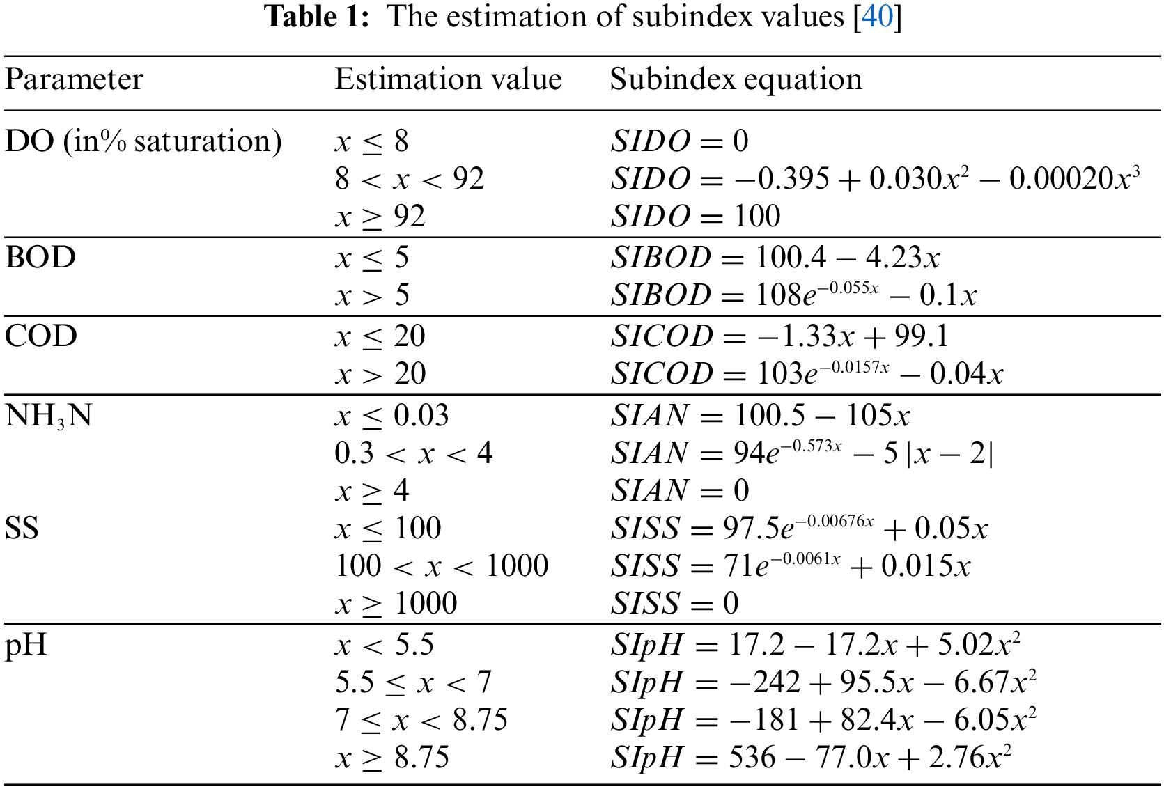
The WQI is calculated by aggregating the subindex values of the input parameters based on Eq. (1) [40] below.

WQI=0.22 SIDO+0.91 SIBOD+0.16 SISS+0.15 SIAN+0.12SIpH (1)

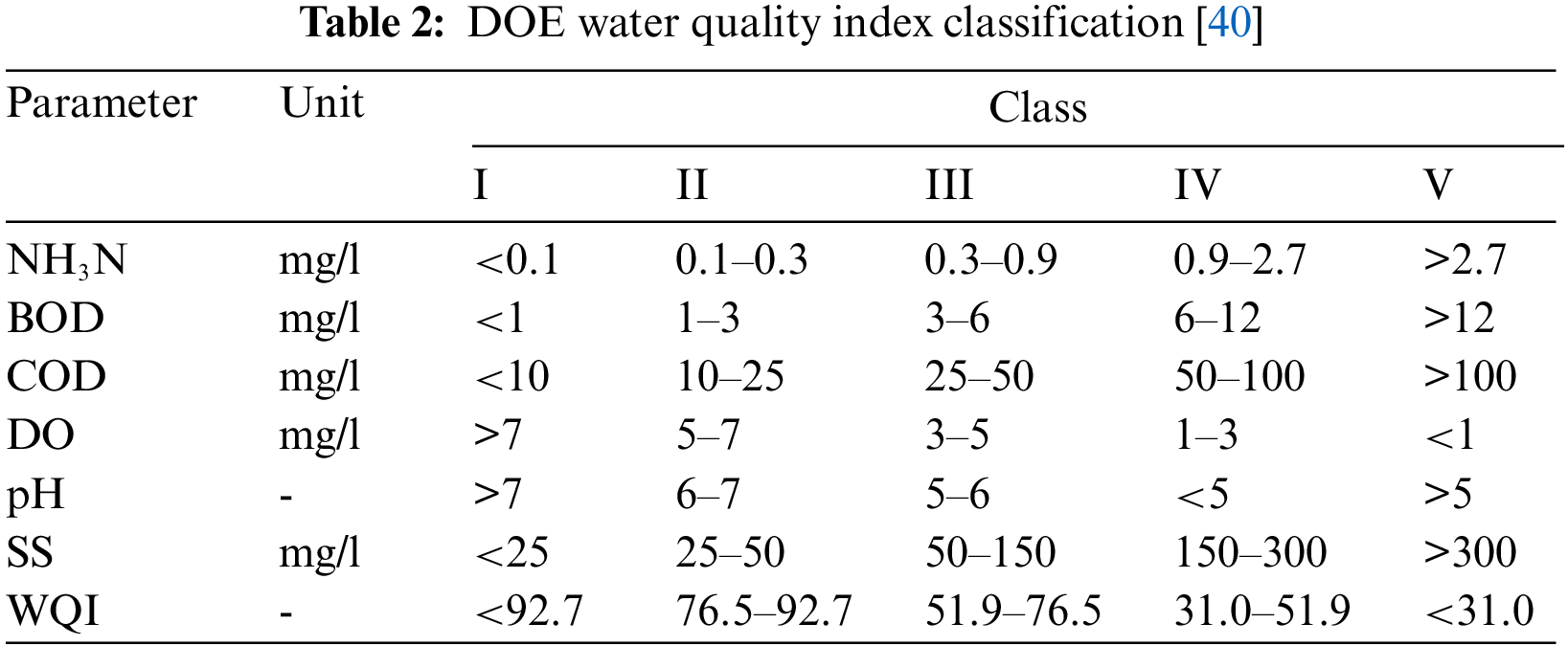
SI denotes the subindex of the input parameters estimated according to Table 1. After adding these sub-indexed values based on Eq. (1), the WQI is then categorized into five classes shown in Table 2, with its uses listed in Table 3.

According to Fig. 1 above, the violin plot describes the distribution of the output data where the curved surface areas represent the density of the Class, the higher the peak, the higher probability; therefore, Class III is the dominant Class, while Class V and Class I are the minority Class. The box plot shows the dataset’s median value in Class III.

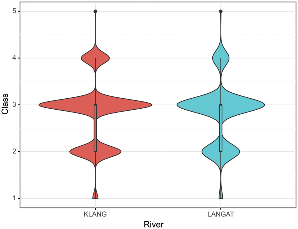
Figure 1: Violin plot of output classes

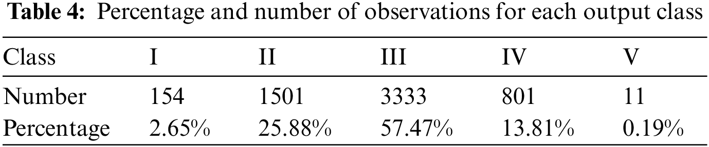
Based on Table 4, there is a significant variance between Class III and Class V, Class III is the daily state of the rivers, while Class V is when heavy pollution has occurred, known as a rare event. The model is exposed to less than 0.19% of training data to identify Class V. From the proportions of Class I, it is deduced that the availability of clean and healthy rivers has gotten scarce and is in decline, while Class II occupies the second-largest fraction of data. Based on the observed data, the river water quality of the Klang and Langat Rivers is still under control, although the most common state of the river exhibits semi-polluted characteristics. Therefore, it is of priority to be able to recognize badly polluted water samples as misclassification of Class V results in human health and ecological risks.

2.2 Stacked Ensemble Deep Learning Generalization

The stacked ensemble methodology improves the model generalization capability [41] as identified by robust prediction performance by researchers [38]. The working concept of stacking is to combine two or more models at level 0, of which a group of predictions is generated that will then act as the input of a meta-learner at level 1 (Fig. 2). At level 0, the input data is fed into several heterogeneous weak learners (sub-models), and the stacking model learns them in parallel. The model maps the ambiguous features between input data as a form of feature extraction. The outputs generated by each sub-model are concatenated as stacked features which will serve as the inputs for level 1. In this second stage, the meta-learner model learns to correct the predictions using the input weak learner’s predictions and the target being the ground truth values. A short script of the pseudocode is presented in Fig. 3. It is summarized that a stacked ensemble obtains a better predictor through several base learners rather than selecting the best predictor.

Figure 2: Stacked ensemble deep learning concept

Figure 3: Pseudocode of the stacked ensemble generalization model

In this study, 23 input variables are inputs to the level 1 sub-models. The model has a single hidden layer with 16 nodes and a rectified linear activation function. The outputs of each sub-model are concatenated and linked to five nodes as the output layer using the softmax activation function, resulting in a single 25-element vector. Because the problem is multi-class, categorical cross entropy is applied as the loss function, and the Adam optimization algorithm is used to optimize the model. It is possible to expand the number of single sub-models at the expense of computational cost. The developed stacked ensemble model is illustrated in Fig. 4 below.

Figure 4: The stacked ensemble deep learning model applied with Keras

2.3 State-of-the-Art (SOTA) Classifiers

SOTA classifiers are machine learning models considered state-of-the-art (SOTA) in their performance on benchmark datasets. These models typically achieve high accuracy, precision, recall, and other performance metrics and are often used as baselines for comparison with other models.

Two examples of SOTA classifiers are XGBoost (eXtreme Gradient Boosting) [42] and Light GBM (Light Gradient Boosting Machine) [43]. Both are gradient-boosting frameworks that use decision trees as base learners. They are particularly effective for handling tabular data and have been used successfully in many real-world applications, including online advertising, credit risk analysis, and fraud detection.

The working formula for XGBoost involves iteratively adding decision trees to the ensemble, with each tree attempting to correct the mistakes of the previous trees. By combining the outputs of many weak learners (i.e., decision trees) in this way, XGBoost can produce a strong learner that can make accurate predictions on new data. In addition, XGBoost has built-in regularization to prevent overfitting, including L1 and L2 regularization and early stopping.

Light GBM employs a technique called ‘gradient-based one-side sampling’ (GOSS), which reduces the number of samples used to calculate the gradients during training by focusing on the samples with the largest gradients. This technique helps to reduce overfitting and speed up training. The Light GBM algorithm uses the histogram-based algorithm for calculating the gains, which is much faster and more memory-efficient than the traditional approach of calculating the exact gains for each split.

Overall, XGBoost and Light GBM are considered to be among the most effective and widely used machine learning models for classification and regression tasks, particularly in the context of tabular data. They have been shown to outperform many other models on a wide range of benchmark datasets, making them an essential tool for data scientists and machine learning practitioners.

2.4 Synthetic Minority Oversampling Technique (SMOTE)

In general, to overcome the issue of imbalanced data, the generation of more training data in the minority class will result in higher performance during machine learning. The SMOTE approach oversamples the data points of minority classes along the line of each point to their k nearest neighbors (as shown in Fig. 5). Thus, it creates more extensive and less specific decision regions of the minority samples [44].

Figure 5: Interpolation of synthetic samples in SMOTE

The SMOTE algorithm generates synthetic random samples by first taking the difference between the feature sample and its nearest neighbor, which is then multiplied by a random number between 0 and 1 before adding the multiplied difference to the feature sample. The SMOTE process creates a selection of random points between two feature samples. The SMOTE approach effectively generalizes the boundary of decisions for the minority class. An example of the algorithm is shown in Fig. 6.

Figure 6: SMOTE pseudocode example [29]

2.5 Performance Metrics

In this study, six performance metrics are evaluated during the training of classifiers, that are: accuracy, precision, recall, F1 score, balanced accuracy, and geometric mean (G-mean). The confusion matrix is calculated to reveal information between the actual and predicted values of the classification models. Based on the output generated, the results are presented in terms of TP, true positives; TN, true negatives; FP, false positives and FN, false negatives. The measure of accuracy is shown in Eq. (2) by taking the total number of true positives and true negatives and dividing it against the total number of the testing data, N.

Accuracy=TP+TNN×100%(2)

The effectiveness of the classification systems is also measured based on their precision, recall, and F1 score. Precision shows the ratio of true positive predictions to the total number of predicted positives. Recall or sensitivity is the ratio between correct predictions and the total number of observations. F1 score is a score balance between precision and recall, whereby a scoring closer to one has the best model performance.

Precision=TPTP+FP(3)

Recall=TPTP+FN(4)

F1 score=2×Precision×RecallPrecision+Recall(5)

Balanced accuracy is calculated as the average of the sensitivity (true positive rate) and specificity (true negative rate) for each class.

Balanced accuracy=Sensitivity+Specificity2(6)

G-mean is defined as each class’s geometric mean of sensitivity and specificity. It is denoted as the square root of the product of sensitivity and specificity.

G−mean=Recall×Specificity(7)

Both balanced accuracy and g-mean are useful metrics for evaluating the performance of classification models on imbalanced datasets. They provide a more balanced view of model performance by considering its performance across all classes in the dataset rather than just focusing on the model’s overall accuracy.

3  Results and Discussion

3.1 Stacked Ensemble Deep Learning Classifier Analysis

The dataset is split into a 70/30 ratio, where 70% of the data is used for training, and 30% is applied for testing. The stacked ensemble deep learning (SE-DL) model in this study comprises a stack of five individual sub-models applied in the first level of the algorithm, which is later fed into the meta-learner. The Google CoLab virtual machine platform is utilized in this study for deep learning training and analysis due to its availability of graphics processing units (GPUs) and Tensor processing units (TPUs) computing resources.

The performance of the SE-DL model is presented in the normalized confusion matrix shown in Fig. 7 as an overview of the frequency between accurate and inaccurate predictions. Based on the diagonal row of values closer to 1 in the figure, it is concluded that the SE-DL model performs reliably in imbalanced water quality index classification.

Figure 7: Confusion matrix of the stacked ensemble deep learning model

3.1.1 Performance Evaluation of Classifiers

Fig. 8 illustrates the performance metrics calculated using confusion matrices for ten machine learning classifiers, three multi-class imbalanced learning methods, and the proposed stacked ensemble deep learning (DL) model trained based on 23 attributes suited for water quality prediction of the study site. The ten classifiers tested consist of the AdaBoost (ADA), Support Vector Machine (SVM), Linear Discriminant Analysis (LDA), k-Nearest Neighbors (kNN), Naïve Bayes (NB), Decision Trees (DT), Random Forest (RF), Extra Trees (ET), Bagging (BAG) and the Multilayer Perceptron (MLP) classifiers, while the three imbalanced learning methods tested are the balanced bagging (BBAG) classifier, Easy Ensemble Classifier (EEC), and the RUSBoost classifier. The RUSBoost algorithm combines RUS (random under-sampling) and the AdaBoost procedure. These classifiers have been adopted in previous literature for water quality classification; therefore, they are used in this study as benchmarks of comparison to the proposed stacked ensemble model.

Figure 8: Performance evaluation of classifiers

The accuracy of each classifier is validated for five runs, with its average accuracy and standard deviation tabulated in Table 5. The 14 models tested are trained on data that has not been pre-processed with SMOTE; to retain the imbalanced data in the system for analysis purposes.

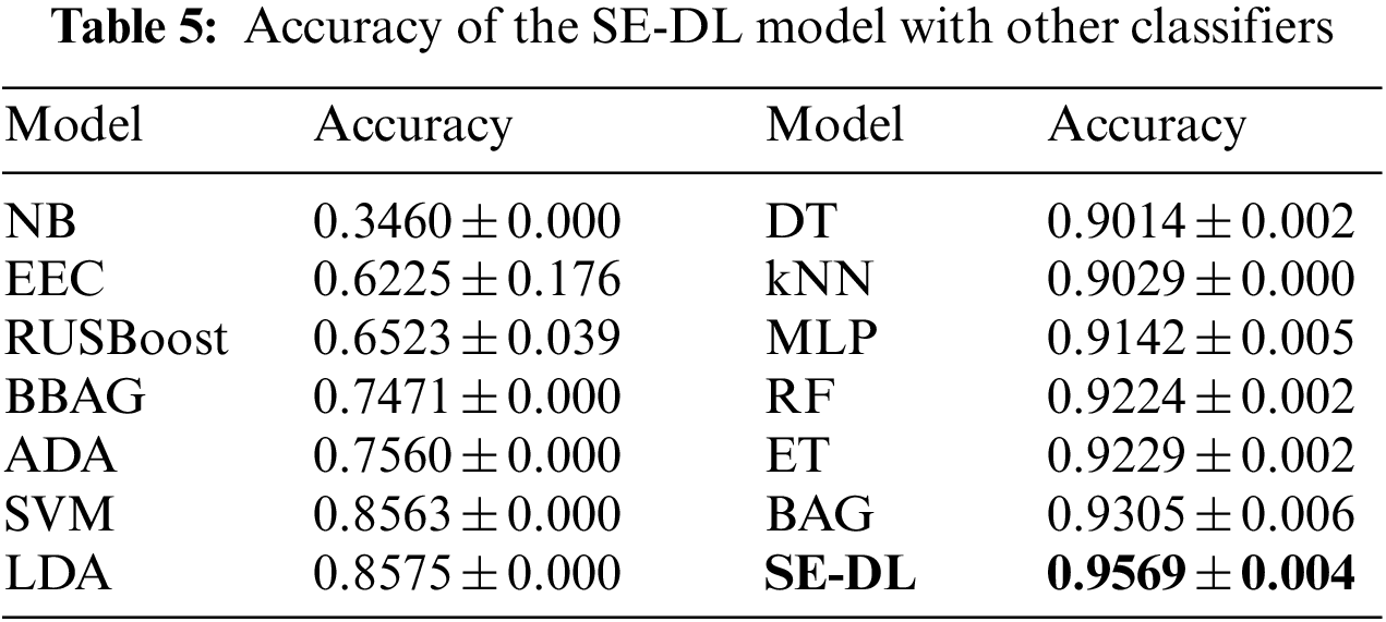
According to the estimates in Table 5, other than the Naïve Bayes classifier, all models return a satisfying accuracy. However, regarding the classifier’s sensitivity and specificity from Fig. 8, most models are underperforming in identifying the minority classes of I and V. This is because the model is well-trained to identify the most frequent observations but not for the rare events. The uncommon samples were regarded as noises to the traditional machine learning classifiers.

All three multi-class imbalanced learning methods do not perform very well. Among all ML classifiers, the ET model is the best in precision, whereas, in overall precision, recall, and accuracy, the Bagging classifier performed the best, followed by the MLP model. However, in this study, the SE-DL model generates the best performance in all four-performance metrics. It can balance the prediction for all five classes well. It is confirmed that the proposed learning algorithm surpasses the traditional machine learning approaches.

3.1.2 Performance Evaluation with SOTA Classifiers

This section compares the performance of the SE-DL model with SOTA classifiers. The two SOTA classifiers applied are the XGBoost and Light GBM algorithms. When comparing the performance of different models, especially when there is imbalanced data, metrics such as balanced accuracy and g-mean can provide a different perspective on the model’s performance. In this case, the SE-DL model has the best accuracy, but the XGBoost classifier has the higher balanced accuracy and g-mean. However, the water quality problem and the trade-offs between precision and recall are also worth considering. Table 6 compares the accuracy, balanced accuracy and g-mean between the SE-DL model with SOTA classifiers. Each classifier is validated for five runs, the performance metrics are tabulated in terms of its average accuracy and standard deviation.

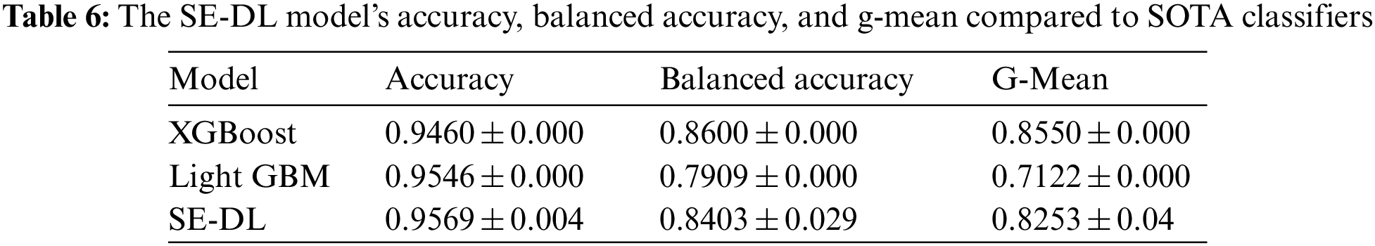
Fig. 9 shows the stacked bar plot of precision, recall, and F1 score between the stacked ensemble DL model, XGBoost (denoted as XGB), and Light GBM (denoted as LGBM) model. It is concluded that the SE-DL model returns better overall precision, recall, and F1 score. When dealing with imbalanced water quality datasets with classes 1–5, where Class 1 represents the best water quality and Class 5 represents the worst water quality, the macro average of precision, recall, and F1 score are important metrics in water quality because they provide a measure of the accuracy and completeness of the model’s predictions for each class, and provide a measure of the overall performance of the model across all classes.

Figure 9: Performance evaluation of SOTA classifiers

Considering all the metrics, while the XGBoost model has the best-balanced accuracy and g-mean, the SE-DL model has higher accuracy, precision, recall, and F1 score. By balancing the precision and recall across all classes, the SE-DL model is the better choice due to its higher F1 score. The F1 score measures the balance between accuracy and completeness for each water quality class.

In water quality, accurate predictions of the water quality class are important for ensuring that the water is safe for drinking, irrigation, or recreational use. While a high precision indicates that the model accurately predicts the correct class for a sample, recall measures the proportion of actual positive samples that are correctly predicted as positive. Both are important metrics to ensure badly polluted samples are not misclassified as slightly polluted.

By using precision, recall, and F1 score to evaluate the model’s performance, it is possible to identify areas where the model is performing well and areas where it needs improvement. It is crucial for water quality experts to make informed decisions about how to manage and protect water resources and ensure that the water is safe for use.

3.1.3 Comparison of the SE-DL Model with or Without SMOTE

SMOTE resampling often improves the model’s reliability in identifying minority classes; it is hypothesized that the system’s accuracy would improve, as well as the precision and recall rate of minority classes, when SMOTE is utilized. The hypothesis is tested in this study for deep learning in a comparative analysis of the proposed stacked ensemble model trained with and without the SMOTE algorithm. First, the SMOTE instance is defined with default parameters. Next, two models are built; Model DL-A represents the model trained under the basic training dataset, while Model DL-B provides the model’s performance that has undergone SMOTE. Finally, both models are tested on the same testing dataset to ensure constancy. The data records per class before and after SMOTE for Model DL-B are shown in Table 7.

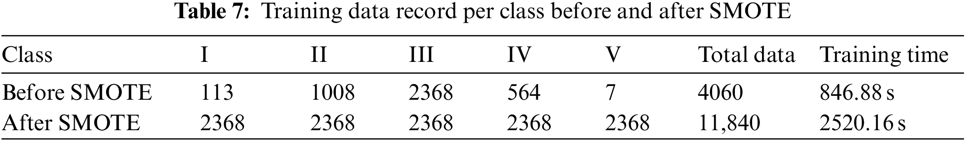
Notably, Model DL-B occupied a longer iteration time to manage its larger sample size resulting from the oversampling of the dataset performed by SMOTE shown in Table 7. Therefore, there are 11,840 rows for training Model DL-B, whereas Model DL-A only has 4060 trainable data. Subsequently, the computational time of Model DL-B is three times more than Model DL-A.

According to Table 8, both deep learning models have performed outstandingly in accuracy, precision, recall, and F1 score. An approximate 0.5% improvement is observed when the deep learning model is tested in Model DL-B, as the accuracy increased from 95.69% in Model DL-A to 96.08%. Comparing the F1 score of each water quality class suggests that both models’ handling abilities on imbalanced data are equally effective and consistently high.

Despite having better prediction performance, the slight increase in performance in Model DL-B is impractical as it requires higher processing power, space, and time to handle the imbalanced dataset. If a larger dataset were to be applied, the model might be unable to converge and thus not adapted for future real-time water monitoring practices. A shorter learning time yet equally accurate prediction of the Model DL-A is sufficient for the application. Thus, the stacked ensemble deep learning model without any SMOTE resampling algorithms (Model DL-A) is effective and preferable for water-quality deep learning analysis.

Furthermore, the setback from learning algorithms involving SMOTE is the increased complexity. It is expected that minority Classes I and V would improve in sensitivity; however, the F1 score of Class I was lower after training with SMOTE in Table 8. The tendency of SMOTE learning models to pose boundary issues is relatively high, which introduces more noise to the system.

Moreover, it is also identified that the sub-individual models in level 0 performed differently, although both models produced similar results after the concatenation phase in level 1. Figs. 10 and 11 below present the learning curves of the sub-individual models in Model DL-A and Model DL-B, respectively. Model DL-A (Fig. 10) showed better stability and less deviation between the training and testing dataset in terms of loss and accuracy. On the other hand, Model DL-B in Fig. 11 demonstrated lower accuracy and a higher loss in the testing dataset, which means the model is underfitting in the training stage, unable to capture the underlying relationship of the dataset with SMOTE.

Figure 10: The learning curves for (a) accuracy and (b) loss of sub-models in Model DL-A

Figure 11: The learning curves for (a) accuracy and (b) loss of sub-models in Model DL-B

3.2 Sensitivity Analysis

In classifier optimization, feature selection continues to pose a challenge for research. Extensive methods and time complexity could trade in with increased model sensitivity. This section concludes the results of the stacked ensemble deep learning algorithm in this section by tabulating the importance of each predictor to the deep learning model in Table 9 below. Sensitivity analysis provides the statistical rankings of each input parameter to generate insights regarding the influence of each predictor.

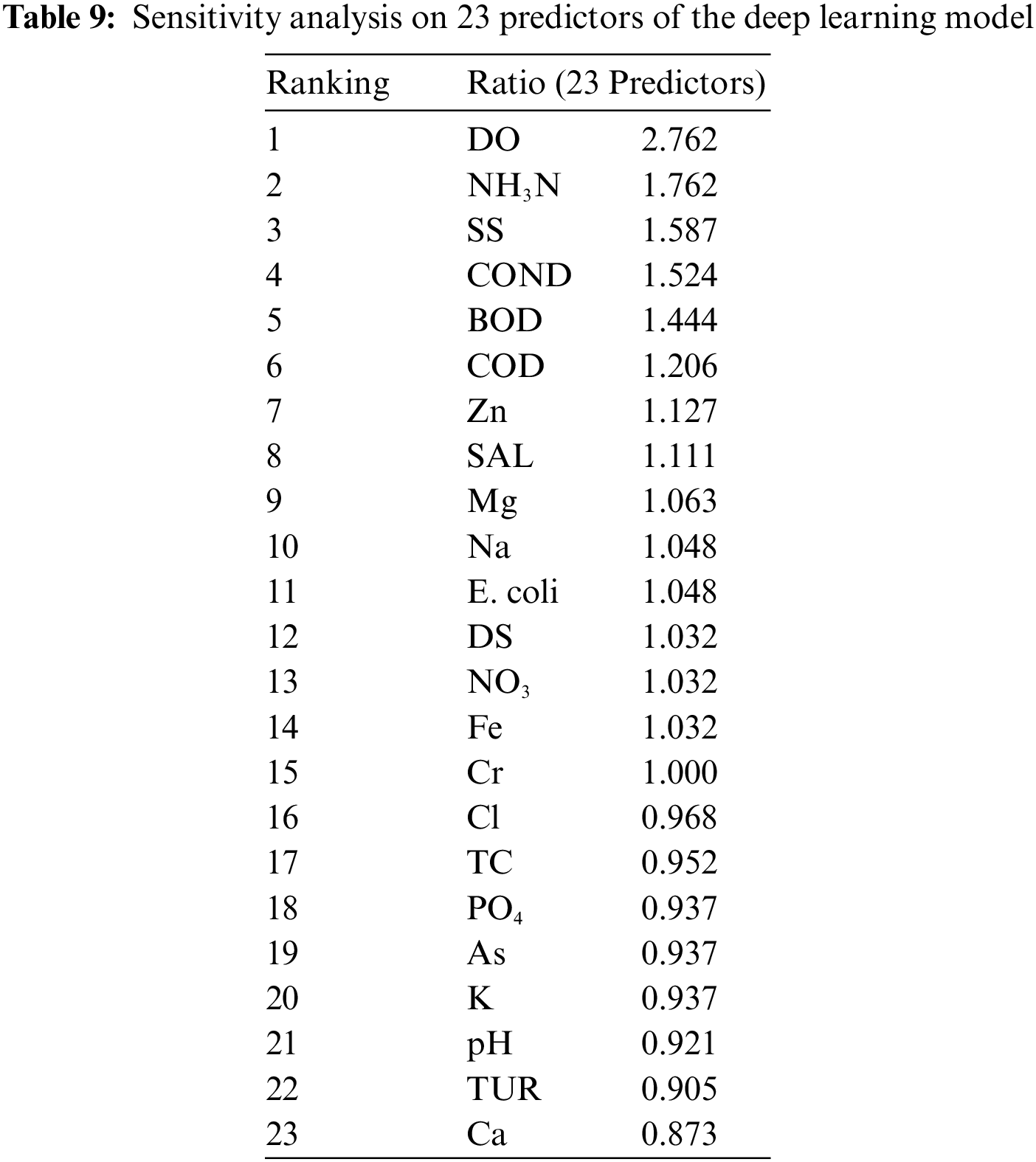
Based on Table 9, pH is low in the ranking, although it is among the index formulation’s six standard water quality (WQ) parameters. Although conductivity is not involved in the water quality index formulation, it possesses more significant influence at ranking four among the 23 predictors. This is because conductivity represents many dependent variables for WQI justified by the number of dissolved salts and organic compounds [45]. When electrical conductivity is high, more impurities are present in water bodies, indirectly influencing the biological levels measured in WQI. These impurities contain ions such as chloride, phosphate, and nitrate from sewage runoff and agricultural waste. The accumulation of these contaminations could deteriorate water quality. For example, concentrated chloride levels could corrode iron pipes [46], while excessive nitrate and phosphate trigger the growth of algae blooms, eventually causing oxygen depletion or ecosystem disruption, known as eutrophication [47,48]. These processes often accumulate in their effects until the dissolved oxygen indicator reflects the unhealthy water system. Furthermore, the microbiological aspects of a river should not be neglected to prevent the occurrence of a waterborne outbreak. Therefore, the inclusion of E. coli sorted to the 11th position of sensitivity towards the deep learning model should be considered in future water quality evaluation systems.

Sensitivity analysis provides insights for feature optimization. When feature optimization was implemented, it involved selecting the most informative features for the prediction model while discarding irrelevant or redundant ones. This helps to improve the accuracy and interpretability of the developed model; by optimizing the input features, water quality prediction models can be made more robust and effective, as they focus on the most critical parameters likely to have the greatest impact on water quality.

3.3 Discussion

This section discusses the findings of this research with other studies in Table 10. Typical applications of ML models include artificial neural network (ANN) through back propagation neural networks (BPNN) and radial basis function neural network (RBFNN) [49], and SVM models [50], in which both studies have proven equally effective for streamlining the computation process of WQI in Langat and Klang River, Malaysia. However, the ANN models are susceptible to overfitting and local minima problems [51], whereas SVMs are complex to build for linearly inseparable classes. Such shortcomings, on the other hand, could be overcome with hybrid optimization and generalization techniques, as demonstrated in this study with the stacked ensemble generalization model. The gradient boosting (GB) method shown by Malek et al. [52] generated a high performance at low classification error. However, Malek, et al. [52] only addressed the imbalanced issue by introducing the metric of balanced accuracy, in contrast to the novelty of this work, where the imbalanced issue is resolved at the algorithm level through stacking.

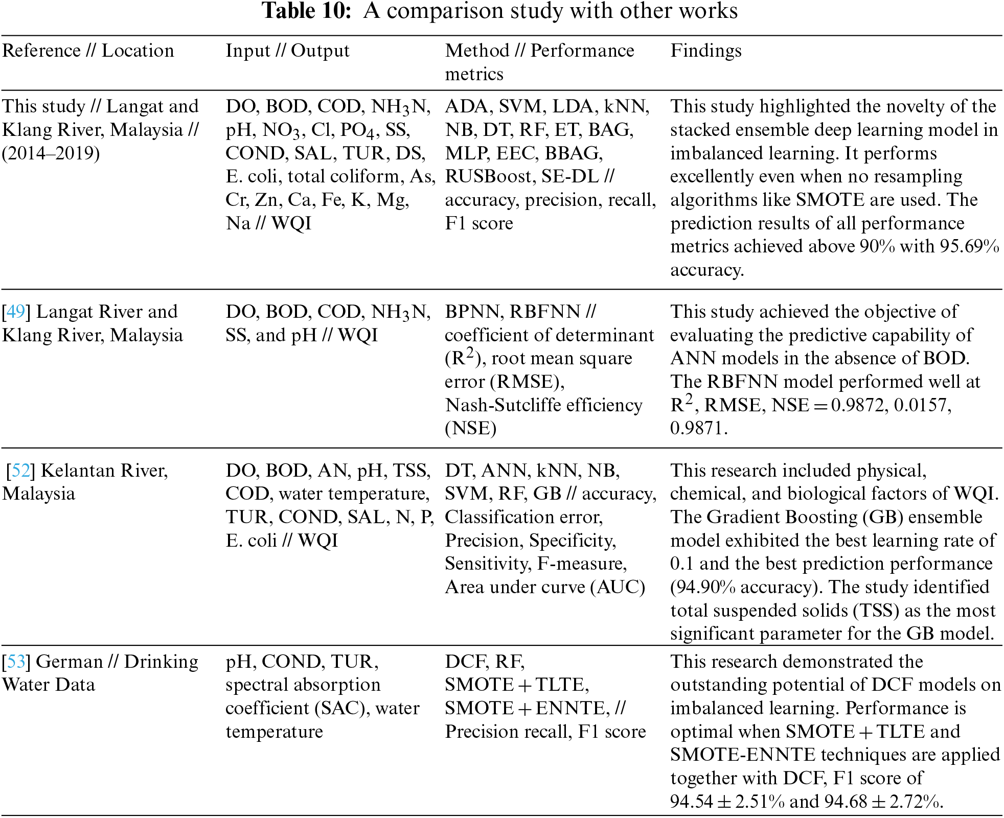
Chen et al. [53] enhanced SMOTE with data cleaning techniques, such as the Tomek links technique (TLTE) or the edited nearest neighbor technique (ENNTE). The study tested 16 different learning models, with the Deep Cascade Forest (DCF) model emerging as the best model. DCF is an emerging deep-learning model constructed by a cascade of random forests. The ability of DCF was proven outstanding, as it could treat data in multiple domains. Combining these sampling techniques would generate a far superior performance in increasing the F1 score. The contributions made from this study are aligned with the methods tested by Chen et al. [53] for imbalanced learning, using deep learning, ensemble, and sampling techniques.

The merit of the stacked ensemble deep learning model in this research is its ability to stand alone without being pre-processed with SMOTE during model training. However, this method poses limitations, such as overgeneralizing a specific water quality dataset. Therefore, a more extensive dataset is requested to train this model. Moreover, despite deep learning’s powerful learning ability, the lack of features may prevent the model from accurately representing the nature of the data. Therefore, the use of 23 inputs is recommended to encompass all aspects of water quality attributes.

This study concludes that deep learning models can handle significant model complexity, such as a dataset of imbalanced nature. It has multiple processing layers optimized for model parameters, neurons, and batch size, making it more efficient in managing massive data. Based on the performance of the stacked ensemble model, it is inferred that the deep learning model is highly competitive even without SMOTE processing of the input dataset. Ensemble models are often adapted to handle more features or larger sample sizes as the training of the ensemble model is disjoint to several embedded individual models designed for feature extraction and transformation to achieve reasonable accuracy [54]. Published work by Ali et al. [55] indicated that feature fusion based on ensemble deep learning improves the prediction of heart diseases. Appropriate addition of input features to the training process could improve the predictive ability of the system [56].

Future work on this can include feature optimization and the stacked ensemble model, which can help policymakers make more informed decisions and take more effective actions to protect and manage water resources. This can lead to better water quality outcomes, improved public health, and more sustainable use of our water resources.

4  Conclusion

The stacked ensemble deep learning (SE-DL) model presented in this study is reliable and robust in predicting an imbalanced water quality index (WQI). This method outperforms traditional machine learning algorithms or SMOTE techniques with reasonable accuracy within a short computation time. Although SMOTE generates better accuracy and performance, the training time with SMOTE was longer. The oversampling algorithm increases the quantity of data to be iterated, resulting in a slight improvement in the effectiveness of water quality prediction when SMOTE is applied; nevertheless, training time increases proportionally due to the increased amount of data to be iterated. To generate a fair value of precision and recall, there is a need for the SMOTE algorithm to be applied with machine learning. However, this work demonstrated a deep learning approach that does not require the implementation of SMOTE, to return a good accuracy of 95.69%. The necessity to balance the skewed distribution in the stacked ensemble deep learning model has been overcome by training the model on two tiers of learning models. The first tier extracts the characteristics of each input, with its output supplied to the second tier of a meta-learner as inputs. This stage eliminates the biases of the majority distribution while weight adjustments are assigned in the hidden layer tuned to the minority instances. It is also verified in this study that accuracy is not the best performance metric for model training in imbalanced data; as proven in this work, ML models high in accuracy may underperform in terms of precision and recall rate.

Moreover, this work thoroughly suggests using more input parameters to better represent water quality assessment. Although it is speculated that increasing the number of features in model training could generate confusion and noise in the system, the deep learning model was able to handle the amount of complexity, thus yielding good results. The interrelation present between water quality variables is one of the factors the deep learning model can discover patterns and relations between each feature. Despite the excellency learning capabilities of deep learning models, a lack of features may prevent the model from accurately representing the nature of the data. This assertion is substantiated by a sensitivity analysis determining the high dominance of dissolved oxygen and ammoniacal nitrogen in deep-learning water quality models.

This study was limited by the availability of data, which was obtained from a single source and only included a small number of minority classes. This could limit the generalizability of the results and make it difficult to evaluate the model as a whole. Moreover, this study did not perform an extensive hyperparameter tuning process, which could lead to the suboptimal performance of the model. As a result, the model may not be as accurate or robust as it could be, as the best set of parameters for the given dataset and problem is not identified.

Therefore, this research can be extended by training the model under a larger dataset with more significant skewed distributions, including catastrophic events from extreme weather, climate change, and human-caused pollution. The proposed stacked ensemble deep learning model is prone to overgeneralizing recent water quality events; exposing the model to a longer time frame improves its ability to anticipate these rare events. Notably, the type and number of variables considered in water quality representation should not be taken lightly, as the negligence of one factor could trigger a potential waterborne disease outbreak. This work acts as a step towards using deep learning stacked ensemble models in addressing challenges from imbalanced water quality data.

Concisely, improvements in water quality prediction can help policymakers manage water quality in several ways.

•   Firstly, more accurate and reliable water quality prediction models can help policymakers identify areas at high risk of contamination and the factors that contribute to water pollution. This can inform the development of targeted interventions, such as improved agricultural practices or implementing management practices for stormwater management.

•   Secondly, the ability of these models to detect and predict water quality issues can help policymakers to prioritize their resources and respond more efficiently to potential water quality problems. This can lead to more effective and timely interventions, such as issuing public advisories or implementing water quality monitoring programs.

•   Thirdly, by optimizing the input features and addressing the class imbalance, water quality prediction models can be more transparent and interpretable. This can improve policymakers’ understanding of water quality factors, allowing for more informed decision-making and policy development.

Acknowledgement: The authors thank the Department of Environment Malaysia (DOE) for the provided data.

Funding Statement: This study is primarily supported by the Ministry of Higher Education through MRUN Young Researchers Grant Scheme (MY-RGS), MR001-2019, entitled “Climate Change Mitigation: Artificial Intelligence-Based Integrated Environmental System for Mangrove Forest Conservation,” received by K.H., S.A.R., H.F.H., M.I.M., and M.M.A. This work is secondarily funded by the UM-RU Grant, ST065-2021, entitled Climate Smart Mitigation and Adaptation: Integrated Climate Resilience Strategy for Tropical Marine Ecosystem.

Availability of Data and Materials: The authors do not have permission to share the data.

Conflicts of Interest: The authors declare they have no conflicts of interest to report regarding the present study.

References

1. D. Hinrichsen and H. Tacio, “The coming freshwater crisis is already here,” in The Linkages Between Population and Water. Washington, DC: Woodrow Wilson International Center for Scholars, pp. 1–26, 2002. [Google Scholar]

2. R. Das Kangabam and M. Govindaraju, “Anthropogenic activity-induced water quality degradation in the Loktak lake, a Ramsar site in the Indo-burma biodiversity hotspot,” Environmental Technology, vol. 40, no. 17, pp. 2232–2241, 2019. [Google Scholar] [PubMed]

3. X. Nong, D. Shao, H. Zhong and J. Liang, “Evaluation of water quality in the south-to-north water diversion project of China using the water quality index (WQI) method,” Water Research, vol. 178, 115781, 2020. [Google Scholar]

4. M. A. Haq, “Planetscope nanosatellites image classification using machine learning,” Computer Systems Science & Engineering, vol. 42, no. 3, pp. 1031–1046, 2022. [Google Scholar]

5. M. A. Haq, “CNN based automated weed detection system using UAV imagery,” Computer Systems Science & Engineering, vol. 42, no. 2, pp. 837–849, 2022. [Google Scholar]

6. M. A. Haq, “SMOTEDNN: A novel model for air pollution forecasting and AQI classification,” Computers, Materials & Continua, vol. 71, no. 1, pp. 1403–1425, 2022. [Google Scholar]

7. G. Revathy, S. A. Alghamdi, S. M. Alahmari, S. R. Yonbawi, A. Kumar et al., “Sentiment analysis using machine learning: Progress in the machine intelligence for data science,” Sustainable Energy Technologies and Assessments, vol. 53, 102557, 2022. [Google Scholar]

8. B. P. S. Kumar, M. A. Haq, P. Sreenivasulu, D. Siva, M. B. Alazzam et al., “Fine-tuned convolutional neural network for different cardiac view classification,” The Journal of Supercomputing, vol. 78, pp. 18318–18335, 2022. [Google Scholar]

9. M. A. Haq, M. A. R. Khan and M. Alshehri, “Insider threat detection based on NLP word embedding and machine learning,” Intelligent Automation & Soft Computing, vol. 33, no. 1, pp. 619–635, 2022. [Google Scholar]

10. S. Khullar and N. Singh, “Water quality assessment of a river using deep learning Bi-LSTM methodology: Forecasting and validation,” Environmental Science and Pollution Research, vol. 29, no. 9, pp. 12875–12889, 2022. [Google Scholar] [PubMed]

11. P. Liu, J. Wang, A. K. Sangaiah, Y. Xie and X. Yin, “Analysis and prediction of water quality using LSTM deep neural networks in IoT environment,” Sustainability, vol. 11, no. 7, 2058, 2019. [Google Scholar]

12. V. V. D. Prasad, L. Y. Venkataramana, P. S. Kumar, G. Prasannamedha, K. Soumya et al., “Water quality analysis in a lake using deep learning methodology: Prediction and validation,” International Journal of Environmental Analytical Chemistry, vol. 102, no. 17, pp. 5641–5656, 2020. [Google Scholar]

13. T. B. Trafalis, I. Adrianto, M. B. Richman and S. Lakshmivarahan, “Machine-learning classifiers for imbalanced tornado data,” Computational Management Science, vol. 11, no. 4, pp. 403–418, 2014. [Google Scholar]

14. S. Makki, Z. Assaghir, Y. Taher, R. Haque, M. Hacid et al., “An experimental study with imbalanced classification approaches for credit card fraud detection,” IEEE Access, vol. 7, pp. 93010–93022, 2019. [Google Scholar]

15. A. M. Richardson and B. A. Lidbury, “Enhancement of hepatitis virus immunoassay outcome predictions in imbalanced routine pathology data by data balancing and feature selection before the application of support vector machines,” BMC Medical Informatics and Decision Making, vol. 17, no. 1, pp. 1–11, 2017. [Google Scholar]

16. C. M. Vong, W. F. Ip, C. C. Chiu and P. K. Wong, “Imbalanced learning for air pollution by meta-cognitive online sequential extreme learning machine,” Cognitive Computation, vol. 7, no. 3, pp. 381–391, 2015. [Google Scholar]

17. X. Chen, H. Liu, F. Liu, T. Huang, R. Shen et al., “Two novelty learning models developed based on deep cascade forest to address the environmental imbalanced issues: A case study of drinking water quality prediction,” Environmental Pollution, vol. 291, 118153, 2021. [Google Scholar]

18. H. Kaur, H. S. Pannu and A. K. Malhi, “A systematic review on imbalanced data challenges in machine learning: Applications and solutions,” ACM Computing Surveys, vol. 52, no. 4, pp. 1–36, 2019. [Google Scholar]

19. G. Haixiang, L. Yijing, J. Shang, G. Mingyun, H. Yuanyue et al., “Learning from class-imbalanced data: Review of methods and applications,” Expert Systems with Applications, vol. 73, pp. 220–239, 2017. [Google Scholar]

20. R. Domingues, M. Filippone, P. Michiardi and J. Zouaoui, “A comparative evaluation of outlier detection algorithms: Experiments and analyses,” Pattern Recognition, vol. 74, pp. 406–421, 2018. [Google Scholar]

21. W. A. Rivera and P. Xanthopoulos, “A priori synthetic over-sampling methods for increasing classification sensitivity in imbalanced data sets,” Expert Systems with Applications, vol. 66, pp. 124–135, 2016. [Google Scholar]

22. N. Nnamoko and I. Korkontzelos, “Efficient treatment of outliers and class imbalance for diabetes prediction,” Artificial Intelligence in Medicine, vol. 104, 101815, 2020. [Google Scholar]

23. J. Tanha, Y. Abdi, N. Samadi, N. Razzaghi and M. Asadpour, “Boosting methods for multi-class imbalanced data classification: An experimental review,” Journal of Big Data, vol. 7, no. 1, pp. 1–47, 2020. [Google Scholar]

24. M. Bach, A. Werner, J. Żywiec and W. Pluskiewicz, “The study of under-and over-sampling methods’ utility in analysis of highly imbalanced data on osteoporosis,” Information Sciences, vol. 384, pp. 174–190, 2017. [Google Scholar]

25. B. Krawczyk, M. Galar, Ł. Jeleń and F. Herrera, “Evolutionary undersampling boosting for imbalanced classification of breast cancer malignancy,” Applied Soft Computing, vol. 38, pp. 714–726, 2016. [Google Scholar]

26. A. Moreo, A. Esuli and F. Sebastiani, “Distributional random oversampling for imbalanced text classification,” in Proc. of the 39th Int. ACM SIGIR Conf. on Research and Development in Information Retrieval, Pisa Italy, pp. 805–808, 2016. [Google Scholar]

27. A. Fernández, S. Garcia, F. Herrera and N. V. Chawla, “SMOTE for learning from imbalanced data: Progress and challenges, marking the 15-year anniversary,” Journal of Artificial Intelligence Research, vol. 61, pp. 863–905, 2018. [Google Scholar]

28. D. Ramyachitra and P. Manikandan, “Imbalanced dataset classification and solutions: A review,” International Journal of Computing and Business Research, vol. 5, no. 4, pp. 1–29, 2014. [Google Scholar]

29. N. V. Chawla, K. W. Bowyer, L. O. Hall and W. P. Kegelmeyer, “SMOTE: Synthetic minority over-sampling technique,” Journal of Artificial Intelligence Research, vol. 16, pp. 321–357, 2002. [Google Scholar]

30. P. Kaur and A. Gosain, “Comparing the behavior of oversampling and undersampling approach of class imbalance learning by combining class imbalance problem with noise,” in ICT Based Innovations. Singapore: Springer, pp. 23–30, 2018. [Google Scholar]

31. J. Vanhoeyveld and D. Martens, “Imbalanced classification in sparse and large behaviour datasets,” Data Mining and Knowledge Discovery, vol. 32, no. 1, pp. 25–82, 2018. [Google Scholar]

32. H. Al Majzoub, I. Elgedawy, Ö. Akaydın and M. Köse Ulukök, “HCAB-SMOTE: A hybrid clustered affinitive borderline SMOTE approach for imbalanced data binary classification,” Arabian Journal for Science and Engineering, vol. 45, no. 4, pp. 3205–3222, 2020. [Google Scholar]

33. J. Sun, H. Li, H. Fujita, B. Fu and W. Ai, “Class-imbalanced dynamic financial distress prediction based on Adaboost-SVM ensemble combined with SMOTE and time weighting,” Information Fusion, vol. 54, pp. 128–144, 2020. [Google Scholar]

34. T. Xu, G. Coco and M. Neale, “A predictive model of recreational water quality based on adaptive synthetic sampling algorithms and machine learning,” Water Research, vol. 177, 115788, 2020. [Google Scholar]

35. A. O. Al-Sulttani, M. Al-Mukhtar, A. B. Roomi, A. A. Farooque, K. M. Khedher et al., “Proposition of new ensemble data-intelligence models for surface water quality prediction,” IEEE Access, vol. 9, pp. 108527–108541, 2021. [Google Scholar]

36. K. Chen, H. Chen, C. Zhou, Y. Huang, X. Qi et al., “Comparative analysis of surface water quality prediction performance and identification of key water parameters using different machine learning models based on big data,” Water Research, vol. 171, 115454, 2020. [Google Scholar]

37. G. Elkiran, V. Nourani and S. Abba, “Multi-step ahead modelling of river water quality parameters using ensemble artificial intelligence-based approach,” Journal of Hydrology, vol. 577, 123962, 2019. [Google Scholar]

38. B. Krawczyk, L. L. Minku, J. Gama, J. Stefanowski and M. Woźniak, “Ensemble learning for data stream analysis: A survey,” Information Fusion, vol. 37, pp. 132–156, 2017. [Google Scholar]

39. M. S. Kumar, M. Z. Khan, S. Rajendran, A. Noor, A. S. Dass et al., “Imbalanced classification in diabetics using ensembled machine learning,” Computers, Materials and Continua, vol. 72, no. 3, pp. 4397–4409, 2022. [Google Scholar]

40. DOE, Environmental Quality Report (EQR) 2008. Kuala Lumpur: Department of Environment, Ministry of Natural Resources and Environment Malaysia, 2008. [Google Scholar]

41. D. Wolpert, “Stacked generalization,” Neural Networks, vol. 5, no. 2, pp. 241–259, 1992. [Google Scholar]

42. T. Chen and C. Guestrin, “Xgboost: A scalable tree boosting system,” in Proc. of the 22nd ACM SIGKDD Int. Conf. on Knowledge Discovery and Data Mining, San Francisco, CA, USA, pp. 785–794, 2016. [Google Scholar]

43. G. Ke, Q. Meng, T. Finley, T. Wang, W. Chen et al., “Light GBM: A highly efficient gradient boosting decision tree,” Advances in Neural Information Processing Systems, vol. 30, pp. 3146–3154, 2017. [Google Scholar]

44. H. Han, W. Y. Wang and B. H. Mao, “Borderline-SMOTE: A new over-sampling method in imbalanced data sets learning,” in Int. Conf. on Intelligent Computing, Hefei, China, pp. 878–887, 2015. [Google Scholar]

45. A. F. Rusydi, “Correlation between conductivity and total dissolved solid in various type of water: A review,” in IOP Conf. Series: Earth and Environmental Science, Bandung, Indonesia, vol. 118, no. 1, 012019, 2018. [Google Scholar]

46. M. Wasim, S. Shoaib, N. Mubarak and A. M. Asiri, “Factors influencing corrosion of metal pipes in soils,” Environmental Chemistry Letters, vol. 16, no. 3, pp. 861–879, 2018. [Google Scholar]

47. R. K. Goswami, K. Agrawal and P. Verma, “Phycoremediation of nitrogen and phosphate from wastewater using Picochlorum sp.: A tenable approach,” Journal of Basic Microbiology, vol. 62, no. 3–4, pp. 279–295, 2022. [Google Scholar] [PubMed]

48. M. Magonono, P. J. Oberholster, A. Shonhai, S. Makumire and J. R. Gumbo, “The presence of toxic and non-toxic cyanobacteria in the sediments of the Limpopo river basin: Implications for human health,” Toxins, vol. 10, no. 7, 269, 2018. [Google Scholar]

49. M. Hameed, S. S. Sharqi, Z. M. Yaseen, H. A. Afan, A. Hussain et al. “Application of artificial intelligence (AI) techniques in water quality index prediction: A case study in tropical region, Malaysia,” Neural Computing and Applications, vol. 28, no. 1, pp. 893–905, 2017. [Google Scholar]

50. A. S. A. Yahya, A. N. Ahmed, F. Othman, R. K. Ibrahim, H. A. Afan et al., “Water quality prediction model based support vector machine model for ungauged river catchment under dual scenarios,” Water, vol. 11, no. 6, 1231, 2019. [Google Scholar]

51. R. G. Perea, E. C. Poyato, P. Montesinos and J. A. R. Díaz, “Optimisation of water demand forecasting by artificial intelligence with short data sets,” Biosystems Engineering, vol. 177, pp. 59–66, 2019. [Google Scholar]

52. N. H. A. Malek, W. F. W. Yaacob, S. A. M. Nasir and N. Shaadan, “Prediction of water quality classification of the kelantan river basin, Malaysia, using machine learning techniques,” Water, vol. 14, no. 7, 1067, 2022. [Google Scholar]

53. X. Chen, H. Liu, X. Xu, L. Zhang, T. Lin et al., “Identification of suitable technologies for drinking water quality prediction: A comparative study of traditional, ensemble, cost-sensitive, outlier detection learning models and sampling algorithms,” ACS ES&T Water, vol. 1, no. 8, pp. 1676–1685, 2021. [Google Scholar]

54. S. Madisetty and M. S. Desarkar, “A neural network-based ensemble approach for spam detection in Twitter,” IEEE Transactions on Computational Social Systems, vol. 5, no. 4, pp. 973–984, 2018. [Google Scholar]

55. F. Ali, S. El-Sappagh, S. M. R. Islam, D. Kwak, A. Ali et al., “A smart healthcare monitoring system for heart disease prediction based on ensemble deep learning and feature fusion,” Information Fusion, vol. 63, pp. 208–222, 2020. [Google Scholar]

56. J. Cai, J. Luo, S. Wang and S. Yang, “Feature selection in machine learning: A new perspective,” Neurocomputing, vol. 300, pp. 70–79, 2018. [Google Scholar]