Improved Shark Smell Optimization Algorithm for Human Action Recognition

1  Introduction

Human Action Recognition (HAR) includes the action recognition of a person through imaging data which has various applications. Recognition approaches can be divided into three categories: multi-model, overlapping categories, and video sequences [1]. This data used for recognition is the major difference between images and video categories. Data in form of images and videos are acquired through cameras in controlled and uncontrolled environments. With the advancement of technology in past decades, various smart devices have been developed which to collect images and video data for HAR, health monitoring, and disease prevention [2]. Different research has been carried out on HAR through images or videos over the last three decades [3,4]. Human visual systems get visual information about an object such as its movement, shape, and its variations. This information is used to investigate the biophysical processes of HAR. Computer vision systems have achieved very good accuracy while catering to different challenges such as occlusion, background clutter, scale and rotation invariance, and environmental changes [5].

HAR depending upon the action complexity can be divided into primitive, single-person, interaction, and group action recognition [6]. The basic movement of a single human body part considers primitive action, a set of primitive actions of one person includes including single-person action, a collection of humans and objects involves in interaction while collective actions performed by a group of people are group actions. Computer vision-based HAR systems are divided into hand-crafted feature-based methods and deep learning-based methods. The combined framework of hand-crafted and deep features is also employed by many researchers [7].

The data plays an important role in efficient HAR systems. The HAR data is categorized into color channels, depth, and skeleton information. Texture information can be extracted from color channels, i.e., RGB which is close to the visual appearance, but illumination variations can affect the visual data [8]. Depth map information is invariant to the lighting changes which is helpful in foreground object extractions. 3D information can also be captured through a depth map, but noise factors should be considered while capturing the depth map. Skeletons information can be gathered through color channels and depth maps, but it can be exploited from environmental factors [9]. HAR systems use different levels of features such as whole data as the input of HAR used in [10]. Apart from features, motion is an important factor that can be incorporated into the feature computation step. It includes optical flow for capturing low-level feature information in multiple video frames. Some researchers included motion information in the classification step with Conditional Random Fields, Hidden Markov Models, Long-Short Term Memory (LSTM), Recurrent Neural Networks (RNN), and 3D Convolutional Neural Networks (CNN) [11–15]. These HAR systems have good recognition accuracy using the most appropriate feature set.

A CNN-based convolutional 3D (C3D) network was proposed in [16]. The major difference between the 3D CNN and the proposed one was that it utilized the whole video as an input instead of a few frames or segmented frames, which makes it robust for large databases. The architecture of the C3D network comprises several layer groups like convolutional layer = 8, maximum pooling layers = 5, fully connected layers = 2, and the last softmax loss layer. UCF 101 dataset was utilized to evaluate the best combination of the proposed network architecture. The best performance achieved by the proposed network was using a 3 × 3 × 3 convolutional filter without updating the other parameter. The researcher came up with RNNs [17] to overcome the limitation action of CNN models of information derivation from long timelapse. RNN has proved robust while extracting time dimension features and has one drawback of gradient disappearance. The mentioned problem is addressed by presenting Long Short-Term Memory Network (LSTM) [18], which utilizes processors to gauge the information integrity and relevance. Normally, input gates, output gates, and forget gates are utilized in the processor. The information flow is controlled by gates in the processor and unnecessary information which requires large memory chunks is stored for long-term tasks.

A ConvNet architecture for the spatiotemporal fusion of video fragments has evaluated its performance on dataset UCF-101 by achieving an accuracy of 93.5% and HMDB-51 by achieving an accuracy of 69.2% [19]. An architecture is proposed to handle 3D signals effectively and efficiently and introduced Factorized Spatio-Temporal Convolutional Network (FSTCN). It was tested on two publicly available datasets UCF-101 and achieved 88.1% accuracy, while achieved 59.0% accuracy on HMDB-51 [20]. In another method, LSTM models are trained to utilize the differential gating scheme, which focuses on the varying gain due to the slow movements between the successive frames, change based on Derivate of States (DoS) and this combined called differential RNN (dRNN). The method is implemented on KTH and MSRAction3D datasets. The accuracy achieved on their datasets is 93.96% and 92.03%, respectively [21].

This article presents an improved form of the Shark Smell Algorithm (SSO), which reduces redundant features. The proposed algorithm utilizes both, SSO and White Shark Optimization (WSO) properties to solve the redundancy issues. The proposed iSSO divides the population into sub-spaces to find local and global optimal features. In the end, these extracted local features are used to optimize global features. Features are extracted using 9 pre-trained CNN models, which are selected based on their top-1 and top-5 accuracies in ImageNet competition. This model is tested on two publicly available datasets UCF-Sports (D1) and Hollywood2 (D2) and it has obtained better results than state-of-the-art (SOTA) methods.

2  Proposed Methodology

In an uncontrolled environment, various viewports, illuminations, and changing backgrounds, traditional hand-crafted features have been proved insufficient [22]. In the age of big data and the evolution of ML methods, Deep Learning (DL) has achieved remarkable results [23–25]. These results have motivated researchers around the globe to apply these DL methods to domains involving video data. The challenge of ImageNet classification drastically changed the dimensions of DL methods, when CNNs made a huge breakthrough. The main difference between CNN methods and local feature-based methods is that CNN iteratively and automatically extracts deep features through its interconnected layers.

2.1 Transfer Learning of Pre-Trained CNN Models

Artificial Intelligence (AI) and Machine Learning (ML) have a sub-domain, called Transfer Learning (TL), which transforms the learned knowledge of one problem (base problem) into another problem (target problem). TL improves the learning of a model through the data provided for the target problem. A model trained to classify Wikipedia text can be utilized to classify the texts of simple documents after TL. A model trained to classify cards can also classify birds. The nature of this problem is the same, which is to classify objects. TL provides scalability to a trained model, which enables it to recognize different types of objects. Since 2015, after the first CNN model, AlexNet [22] was proposed, a lot of CNN architectures were proposed. The base for all these models was a competition, where a dataset, ImageNet [26], having 1000 classes was presented. The efficiency of all proposed CNN models to date is still measured on how the proposed model performs on the ImageNet dataset. In this research, nine of the most used CNN models are selected, where, through TL, features of input images from selected datasets will be extracted. Table 1 lists all selected CNN models along with their depth, size, input size, number of parameters, and their top-1 and top-5 accuracies on ImageNet datasets.

2.2 Improved Shark Smell Optimization (iSSO)

The meta-heuristic model used in this article is an improved form of Shark Smell Optimization (SSO) [33]. The SSO was proposed after inspiration was taken from the species of sharks. Sharks are considered as most hazardous and strongest predacious in the universe [34]. Sharks are creatures with a keen ability to smell and highly contrasted vision due to their sturdy eyesight and powerful muscles. They have more than 300 sharp, pointing, and triangular teeth in their gigantic jaws. Sharks usually strike with a large and abrupt bite of prey, which proves so sudden that the prey cannot avoid it. These sharks hunt the prey by using their extreme sense of smelling and hearing the traits of prey. The iSSO algorithm initially divides the whole search space into ȿ subparts. The algorithm then performs the local and global search to find the optimum prey in both, local and global search spaces of ȿ. Once an optimum prey is located, the search then continues to find all the optimal prey in the remaining subparts. The process mentioned below is for a single subpart. The whole process will be repeated for all ȿ. Another factor is the quantity of selected optimal features. For this, ȿ denotes the total selected features.

2.2.1 Prey Tracking

Sharks wander in the ocean freely just like any other organism of the sea and search for prey. In that search, sharks update their positions by the traits of prey. They apply all their tricks to locate, stalk and track down the prey. All senses of sharks along with their average distance range are illustrated in Fig. 1. All these illustrated features help them to exploit and search the whole space for hunting prey.

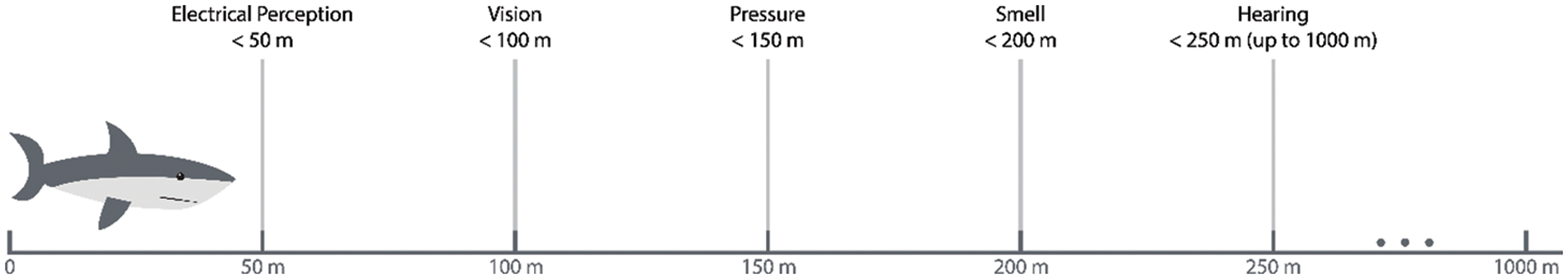
Figure 1: Senses of shark along with its average distance range

2.2.2 Prey Searching (Exploration and Exploitation)

The sharks have a very unfamiliar sense of hearing, that is, they can hear any wavelength from the full length of their body. Their whole body can detect any change in water pressure and reveal the nearby movements of the targeted prey. The attention of sharks is usually attained by moving prey, which leaves a disturbance in water pressure. Sharks even have body organs, which can detect the tiny electromagnetic fields, produced through the swimming of prey. Turbulence due to the prey’s motion helps sharks to sense the frequency of waves and accurately predict the size and location of prey. The velocity of waves detected by sharks is described as:

υ=ω×ωf(1)

where υ denotes the velocity of wavy motion, ω denotes the wavelength that defines the distance between shark and prey and ωf denotes the frequency of waves during the wavy motion. This frequency is determined by the total number of cycles, completed by the shark in a second. The sharks utilize their extraordinary sense to exploit the whole space and to detect prey. Once, a prey is in the nearby area, the senses of the shark grow exponentially, and it travels towards the pined point position of the prey. The following equation is assumed to be used to update the position of a shark with constant acceleration:

ρ=ρi+(υi×ΔT)+(0.5×Acc×ΔT2)(2)

here, a new position of the shark is denoted by ρ, the primitive position is denoted by ρi and the initial velocity is denoted by υi. The interval taken to travel between current and initial positions is represented by ΔT and Acc denotes the constant acceleration factor. Many preys disburse their scent when they leave their position. When a shark reaches that position, it finds no prey and thus starts to search for the prey randomly and explore the nearby areas by using its sense of smell, hearing, and sight. The first step of this algorithm is to generate a search space of all possible solutions. Search space of m sharks in n dimensions, with a position of all sharks, is presented as:

P =[P 11…P n1⋮⋮⋮P 1m…P nm](3)

here, P  is a 2D matrix, containing the positions of all sharks in search space, n denotes the total number of decision variables and P ni represents xth shark in nth dimension. This population is generated by randomly initialized upper and lower bounds as:

P yx=LBy+(rand×(LBy−UBy))(4)

here, P yx denotes the initial matrix of xth shark in the yth dimension, while LBy and UBy denotes the lower and upper bounds of search space in the yth dimension. rand is a randomly generated number between the intervals [0,1]. A fitness function assesses each possible solution for every new position of a shark. If a better position is found, then the current position is renovated with the better one, else the shark remains at its current position.

Now is the time for the shark to move toward prey. When a shark detects the waves of moving prey, it locks its target and starts moving towards that prey, which is defined as:

ρυs+1a=Λ[υsa+ς1(P gbs−P sa)×rand1+ς2(P bυas−P sa)×rand2](5)

In the above equation, a=1,…x denotes the selected shark in search space of size x, the velocity of ath shark in (s+1) steps denoted by υs+1a, υsa is the velocity of ath shark in sth step, P sa is the current position of ath shark in sth step, P gbs is the current global best position of the ath shark in sth iteration, P bυas is the last known best position of the shark, while υa represents an index vector of the best-positioned shark at ith index. rand1 and rand2 are two randomly generated numbers, while ς1 and ς2 denotes the force element on sharks, which controls the impact of P gbs and P bυas, respectively. Λ denotes the factor for constriction. υ and Λ are calculated as per the following equations, respectively:

υ=⌊a×rand(1,a)⌋+1(6)

Λ=2|2−C−C2−4C|(7)

here, C represents the coefficient of acceleration. The value of C for this work is equal to 2.145 after extensive experiments. ς1 and ς2 are calculated as:

ς1=ςmax+(ςmax−ςmin)×e−(4sS)2(8)

ς2=ςmin+(ςmax−ςmin)×e−(4sS)2(9)

here, maximum, and current iterations are denoted by S and s. Active motion of sharks can be achieved by using subordinate and initial velocities denoted by ςmax and ςmin. For this work, these velocities for ςmax and ςmin is set at 0.14 and 1.35, respectively.

The sharks spend most of their time searching for optimal prey and to achieve it, they constantly change their positions. Their position changes when either they smell the scent of prey or they feel the movement in waves, caused by prey. Sometimes, a potential prey leaves its position and leaves some scent, either they feel a shark coming towards them or in search of food. In this case, the shark starts to stray randomly in search of other prey. The position of the shark, in that case, is updated as per the following equation:

P s+1a={P sa⋅∼⊕P 0+UB⋅g+LB⋅h;rand<mFP sa+υsaωf;rand≥mF(10)

here, P s+1a denotes the newly taken position of ath shark in the (s+1)th iteration, ∼ represents the complement operator, g and h represent two 1D binary vectors, P 0 is a logical vector, ωf is the frequency, while movement force denoted by mF is a factor to denote the senses of shark, i.e., smell and hear, which increases with the increasing number of iterations. ⊕ denotes a bitwise xor operation. g, h, P 0, ωf and mF is defined as:

g=scd(P sa−UB)>0(11)

h=scd(P sa−LB)<0(12)

P 0=g⊕h(13)

ωf=ωfmin+ωfmax−ωfminωfmax+ωfmin(14)

mF=1(p+e(0.5×S)−sq)(15)

P s+1a`=P gbs+(rand1×dist→)(scd(rand2−0.3))(16)

dist→=|rand×(P gbs−P sa)|(17)

The Sense is a parameter, which denotes the key senses of a shark while moving towards the prey and it is defined as:

Sense=|1−e−r×sS|(18)

here, r is a positive constant, which is used to manage the behavior of exploitation and exploration of sharks. During the evaluation of this study, the value of r is kept at 0.002.

The behavior of sharks is simulated mathematically by preserving the initial two optimal solutions and updated white shark position w.r.t these optimum solutions. The following equation is used to preserve the stated behavior:

P s+1a=P sa+P s+1a2×rand(19)

This relation shows that the position of the shark is always updated w.r.t. the optimal position of prey. The final location of the shark will be somewhere in the search space, near the optimum prey. The final algorithm of iSSO is presented in Algorithm 1.

After extensive experiments, the value of ȿ and ₣ is set at 14 and 0.65. The impact of these values is also presented in the result section.

3  Experimental Results

The proposed iSSO algorithm is evaluated by performing multiple experiments under different parameters, which efficiently verifies the performance of this algorithm. This section provides an in-depth view of performed experiments along with ablation analysis and comparison with existing techniques.

3.1 Experimental Setup and Datasets

The proposed iSSO algorithm is evaluated on two (2) benchmark datasets including UCF-Sports Dataset (D1) [35] and Hollywood2 Dataset (D2) [36]. D1 contains a total of 150 videos from 10 classes included in this dataset, which represents human actions from different viewpoints and a range of scenes. D2 contains a total of 1,707 videos across 12 classes. These videos are extracted from 69 Hollywood movies.

The proposed iSSO model is trained, tested, and validated using an HP Z440 workstation having an NVIDIA Quadro K2000 with a GPU memory of 2 GB DDR5. This card has 382 CUDA cores along with a 128-bit memory interface and 17 GB/s memory bandwidth. MATLAB2021a was used for training, testing, and validation. All selected pre-trained models are transfer learned with an initial learning rate of 0.0001 with an average decrease of 5% after 7 epochs. The whole process has 160 epochs and overall momentum of 0.45. Selected datasets are split using the standard 70-15-15 ratio for training, testing, and validation. During the testing of the proposed model, eight (8) classifiers were trained, which include Bagged Tree (BTree), Linear Discriminant Analysis (LDA), three kernels of k-Nearest Neighbor (kNN), i.e., Ensemble Subspace kNN (ES-kNN), Weighted kNN (W-kNN) and Fine kNN (F-kNN), and three kernels of Support Vector Machine (SVM), i.e., Cubic SVM (C-SVM), Quadratic SMV (Q-SVM) and Multi-class SVM (M-SVM). The performance of the proposed iSSO algorithm is evaluated using six metrics, such as Sensitivity (Sen), Correct Recognition Rate (CRR), Precision (Pre), Accuracy (Acc), Prediction Time (PT), and Training Time (TT). All experimental results presented in the next section are achieved after performing each experiment at least five times, using the same environment and factors.

3.2 Recognition Results

The efficiency of the proposed model is evaluated by performing multiple experiments. Initially, the impact of all selected pre-trained models is noted by feeding the dataset and extracting features from the selected output layer. In the next experiment, the proposed iSSO algorithm is employed on extracted deep features. And finally, the iSSO-enabled CNN model with the highest accuracy is further forwarded to the other classifiers. It is noteworthy that all the selected classifiers were used during this experiment, but F-kNN achieved the highest accuracy, thus Table 2 contains the results of F-kNN. While using D1, the Na model achieved the highest average Acc of 97.44 was achieved. This average accuracy has a factor, of ±1.36%, which it alters during the five experiments. Similarly, Na obtained 96.97% CRR. The F-kNN took 206 min on average to train and 0.53 s to predict an input image. The lowest average Acc of 73.02% was obtained by the Vg model, whereas Ef took the highest TT of 347 min.

Once a model with the best performance is selected in the first experiment, this model is used to train all selected classifiers. As mentioned earlier, F-kNN performed better on D1 when Na was selected as the base CNN model. This classifier achieved average Sen of 97.37%, an average CRR of 96.97%, and a Pre of 97.28%. The second-best average Acc of 91.75% was achieved by Es-kNN. The worst-performing classifier was BTree, which could only achieve an 80.83% average Acc. The lowest average TT was of 193 s and the lowest average PT of 0.39 s was taken by LDA, but it could only achieve 84.16% Acc.

The proposed model is also evaluated on D2, where the Da network achieved a maximum average Acc of 80.66%. The change factor of this model is 1.04%, after performing the same experiment 5 times. The average CRR of this model is noted at 79.68%. The best classifier for this model is M-SVM, which took 139 min on average to train and 0.48 s on average to predict an input image. The second-best average Acc of 78.27% is achieved by De, which also achieves 78.66% CRR. For this model, M-SVM took 221 min to train and 0.54 s to predict. The lowest average accuracy of 60.02% on D2 is again achieved by Vg, where the selected classifier took 297 min to train and 1.45 s to predict an input image. The performances of all selected CNN models with and without the iSSO algorithm are compared in Table 3.

After the selection of the best-performing CNN model, all selected classifiers are trained on the extracted features of that CNN model. During this experiment, selected evaluation matrices are used to note the performance of each classifier. M-SVM has achieved the best average Sen of 79.22%, best average CRR of 79.68%, best Pre of 79.84%, and best average Acc of 80.66%. This classifier requires 280 min for training and 0.48 s for predicting an input image. The second-best average Acc of 75.88% is obtained by W-kNN, which took 280 min to train and 0.36 s to predict. The lowest TT is noted at 115 min for BTree, but the achieved average Acc is 50.95%.

3.3 Ablation Analysis of iSSO

This section discusses the importance of selecting values of parameters used in the iSSO algorithm. It should be noted that all readings of this section are performed using the network, which obtained the highest accuracy for each dataset, i.e., Na for D1 and Da for D2. Secondly, the classifier used for this analysis is also retrieved from the best experiment for each dataset, i.e., f-kNN for D1 and M-SVM for D2. All experiments in this analysis are performed thrice and an average reading of three experiments is mentioned against each parameter.

The first and most important factor of the iSSO algorithm is the number of subparts ȿ, into which the whole search space, the feature vector, is divided. Table 4 represents the impact of different values for this parameter on accuracy and training time. It is noteworthy that the less value of ȿ decreases TT but reduces the performance of the algorithm.

Another important parameter is ₣, which selects the total number of features after the completion of an algorithm. The impact of ₣ on TT and Acc is shown in Table 5. It is visible that with the increase of selected features, the Acc and TT increase for both datasets until the value of ₣ reaches 0.65.

The coefficient of acceleration C determines how quickly the shark will move from its current position. The quicker the movement is, the less exploration it will make. The acceleration must neither be too fast nor too slow, as the faster shark will skip important and potential prey and slower sharks will take too much time in exploration. Another factor is the behavior of sharks r during the exploitation and exploration process. The value of r determines the intervals, by which each prey should be searched for. Lesser value of r will increase the searching time and ultimately increases the TT. Table 6 represents the comparison of different values of C and r.

The values of ςmax, ςmin, ωfmax and ωfmin do not majorly impact the overall performance of iSSO, specifically in terms of Acc and TT. At the selected values of these parameters, the iSSO has obtained the highest possible performance. Tweaking these parameters marginally changes the results, which can be ignored. The validation accuracy and validation loss of the proposed model on both datasets are shown in Fig. 2, where Figs. 2a and 2b are the validation accuracy and validation loss on D1, respectively, while Figs. 2c and 2d are the validation accuracy and validation loss on D2, respectively. It can be seen that 50% accuracy on both datasets is achieved on the initial 40 epochs, the validation loss is also reduced to less than 50% in the same number of epochs, which shows the high convergence of the proposed model.

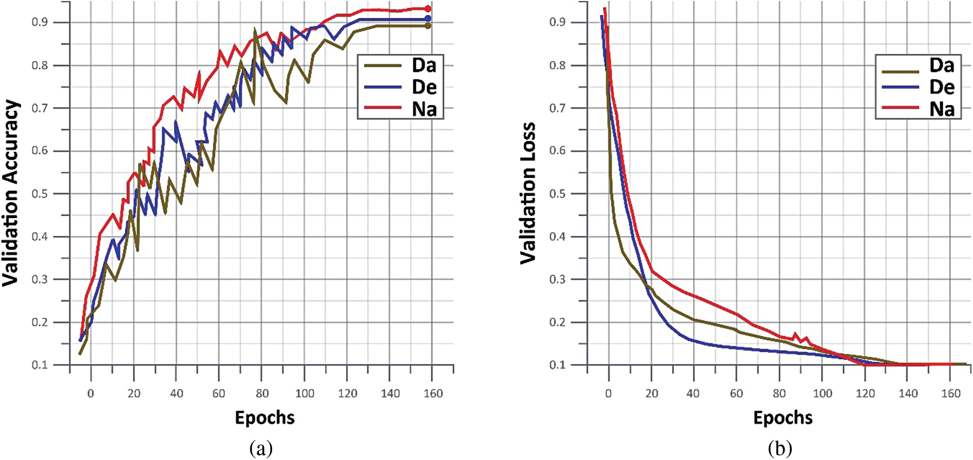
Figure 2: Validation accuracy and validation loss on D1 and D2

3.4 Comparison with Existing Techniques

A hybrid model was proposed in [37] by combining Speeded Up Robust Features (SURF) and Histogram of Oriented Gradients (HOG) for HAR. This model was cable of extracting global and local features as it obtained motion regions by adopting background subtraction. Motion edge features, effectively described by the directional controllable filters were utilized in HOG to extract information on local edges. The bag of Word (BoW) model was also obtained by performing k-means clustering. In the end, Support Vector Machines (SVM) were used to recognize the motion features. This model was tested on SBU Kinect Interaction, UCF Sports, and KTH datasets and achieved accuracies of 98.5%, 97.6%, and 98.2%, respectively. QWSA-HDLAR model was proposed in [38] for the recognition of human actions. This model utilized TL-enabled CNN architecture, called NASNet for feature extraction. The NASNet model also employs a tuning process for hyper-parameters to optimally increase performance. In the end, a hybrid model containing CNN and RNN, called CNN-BiRNN, was used to classify different human actions. This model was tested on D1 and KTH, and it achieved an average recognition rate of 99.0% and 99.6% on both datasets, respectively.

An attention mechanism based on bi-directional LSTM (BiLSTM) and dilated CNN (dCNN) was proposed in [39], which extracted effective features of the HAR frame. Salient features were extracted using the dCNN and these features were fed to the BiLSTM model for the learning process. The learning process helped the model for long-term dependencies, which boosted the evaluation performance and extracted HAR-related cues and patterns. This model was evaluated on J-HMDB, D1, and UCF11 and achieved 80.2%, 99.1%, and 98.3% accuracies, respectively. A DCNN-based model was proposed in [40], which took the input of globally contrasted frames. The resnet-50 model was transferred and learned and it extracted features from a fully connected and global average pooling layer. Both features were fused using Canonical Correlation Analysis (CCA) and then fine-tuned using the Shanon Entropy-based technique. The proposed model was tested on KTH, UT-Interaction, YouTube, D1, and IXMAS datasets and achieved accuracies of 96.6%, 96.7%, 100%, 99.7%, and 89.6%, respectively. The authors in [41] proposed the HAR model using feature fusion and optimization techniques. Before feature engineering, the color transformation was applied to enhance the video frames. Optical flow extracted the moving region after the frames fusion, and these regions were forwarded to extract texture and shape features. Finally, weighted entropy was utilized to select related features and M-SVM was used to classify the actions. This model experimented on UCF YouTube, D1, KTH, and Weizmann datasets and it achieved 94.5%, 99.3%, 100%, and 94.5%, respectively. Table 7 compares the proposed model with existing techniques.

HAR was carried out using three models in [44] including where extraction of compact features, re-sampling of shot framerate, and detection of the shot boundary. The main objective of this research was to emphasize the extraction of relevant features. This model was tested on Weizmann, UCF, KTH, and D2 datasets using the second model, it achieved 97.8%, 95.6%, 97.0%, and 73.6% accuracies, respectively. A lightweight deep learning model was proposed in [45], which recognizes human actions using surveillance streams of CNN models. An ultra-fast object recognizer named Minimum-Output-Sum-of-Squared-Error (MOSSE) locates the subject in a video, while the LiteFlowNet CNN model was used to extract pyramid convolutional features of successive frames. In the end, Gated Recurrent Unit (GRU) was trained to perform HAR. Experiments were conducted on YouTube, Hollywood2, UCF-50, UCF-101 and HMDB51 datasets and overall average accuracy of 97.1%, 71.3%, 95.2%, 95.5% and 72.3%, respectively.

Double-constrained BOW (DC-BOW) was presented in [46], which utilized spatial information of features on three different scales including hidden scale, presentation scale, and descriptor scale. Length and Angle Constrained Linear Coding (LACLC) methods were obtained by constructing a loss function between local features and visual words. To optimize the features, spatial differentiation between extracted features of every cluster was considered. LACLC and a hierarchical weighted approach were applied to extract the related features. The proposed model was tested on UCF101, D2, UCF11, Olympic Sports, and KTH datasets and it achieved accuracies of 88.9%, 67.13%, 96%, 92.3%, and 98.83%, respectively. A Spatiotemporally Attentive 3D Network (STA3D) was proposed in [42] for the propagation of important temporal descriptors and refining of spatial descriptors in 3D Fully Convolutional Networks (3D-FCN). To refine spatial descriptors and propagate temporal descriptors, an adaptive up-sampling module was also proposed. This technique was evaluated on D1 and D2, where it achieved 90% and 71.3% accuracies, respectively. A DCNN-based model is proposed in [43], which has three modules, reasoning and memory, attention, and high-level representation modules. The first modules concentrated on temporal and spatial reasoning so that temporal and spatial patterns could be efficiently discriminated. The second and third modules were mainly utilized for learning through captured spatial saliencies. This model was evaluated on D1 and D2, where it achieved 88.9% and 78.9% accuracies. Table 8 compares the performance of the proposed model with existing techniques.

4  Conclusion

In this article, an analysis of pre-trained CNN models is presented, where 9 models are selected based on their total parameters, size, and Top-1 and Top-5 accuracies. These selected pre-trained CNN models are trained on the selected dataset using the TL. The output layer of these pre-trained models is mentioned, and no experiments are performed based on a selection of the output layer. The extracted features of these CNN models are forwarded to the proposed iSSO, which is an improved algorithm from the traditional SSO. The iSSO algorithm divides the feature vector into subsets, where each subset is then used to find the local and global best features. The selection of local and global best features is inspired by the searching capabilities of the white shark, which uses its senses to find the optimal prey. Once the features are selected, the results are taken using selected publicly available datasets. The limitation of this work is the training time, which is too high, i.e., the lowest training time for D1 is 194 min and for D2, it is 139 min. The one reason for taking this much TT is the dataset, which includes videos. But the main reason is the architecture of these models, which have too many repeated blocks of layers, which can be reduced. In the future, the architecture of the best-performing CNN models of this article will be analyzed to detect and reduce the repeated blocks of layers. The impact of these repeated blocks can also be analyzed.

Acknowledgement: Not applicable.

Funding Statement: This work was supported by the Collabo R&D between Industry, Academy, and Research Institute (S3250534) funded by the Ministry of SMEs and Startups (MSS, Korea), the National Research Foundation of Korea (NRF) grant funded by the Korea government (MSIT) (No. RS-2023-00218176), and the Soonchunhyang University Research Fund.

Author Contributions: The authors confirm their contribution to the paper as follows: study conception and design: I.M.N, M.A.K, and M.R; data collection: I.M.N, M.A.K, and M.R; draft manuscript preparation: I.M.N, M.A.K, M.R, and J.H.S; funding: J-C.N and Y.N; validation: JH.S, Y-C.N, and Y.N; software: I.M.N, M.A.K, Y.N, and Y-C.N; visualization: JH.S, Y-C.N, and Y.N; supervision: M.A.K, M.R and Y.N. All authors reviewed the results and approved the final version of the manuscript.

Availability of Data and Materials: The dataset used in this work is publically available for research purpose.

Conflicts of Interest: The authors declare that they have no conflicts of interest to report regarding the present study.

References

1. V. Sharma, M. Gupta, A. K. Pandey, D. Mishra and A. Kumar, “A review of deep learning-based human activity recognition on benchmark video datasets,” Applied Artificial Intelligence, vol. 36, no. 1, pp. 1–17, 2022. [Google Scholar]

2. S. K. Yadav, K. Tiwari, H. M. Pandey and S. A. Akbar, “A review of multimodal human activity recognition with special emphasis on classification, applications, challenges and future directions,” Knowledge-Based Systems, vol. 223, no. 11, pp. 51–83, 2021. [Google Scholar]

3. I. M. Nasir, M. Raza, J. H. Shah, S. H. Wang, U. Tariq et al., “HAREDNet: A deep learning based architecture for autonomous video surveillance by recognizing human actions,” Computers and Electrical Engineering, vol. 99, no. 1, pp. 1–16, 2022. [Google Scholar]

4. M. Raza, J. H. Shah, M. A. Khan and A. Rehman, “Human action recognition using machine learning in uncontrolled environment,” Artificial Intelligence and Data Analytics, vol. 12, no. 3, pp. 182–187, 2021. [Google Scholar]

5. P. Pareek and A. Thakkar, “A survey on video-based human action recognition: Recent updates, datasets, challenges, and applications,” Artificial Intelligence Review, vol. 54, no. 3, pp. 2259–2322, 2021. [Google Scholar]

6. A. Sarkar, A. Banerjee, P. K. Singh and R. Sarkar, “3D human action recognition: Through the eyes of researchers,” Expert Systems with Applications, vol. 1, no. 2, pp. 11–42, 2022. [Google Scholar]

7. I. U. Khan, S. Afzal and J. W. Lee, “Human activity recognition via hybrid deep learning based model,” Sensors, vol. 22, no. 1, pp. 323–349, 2022. [Google Scholar] [PubMed]

8. Z. Fu, X. He, E. Wang, J. Huo, J. Huang et al., “Personalized human activity recognition based on integrated wearable sensor and transfer learning,” Sensors, vol. 21, no. 3, pp. 885–903, 2021. [Google Scholar] [PubMed]

9. H. Wang, B. Yu, K. Xia, J. Li and X. Zuo, “Skeleton edge motion networks for human action recognition,” Neurocomputing, vol. 423, no. 3, pp. 1–12, 2021. [Google Scholar]

10. Y. B. Cheng, X. Chen, D. Zhang and L. Lin, “Motion-transformer: Self-supervised pre-training for skeleton-based action recognition,” Multimedia Tools and Applications, vol. 4, no. 1, pp. 1–32, 2021. [Google Scholar]

11. K. Liu, L. Gao, N. M. Khan, L. Qi and L. Guan, “Integrating vertex and edge features with graph convolutional networks for skeleton-based action recognition,” Neurocomputing, vol. 466, no. 13, pp. 190–201, 2021. [Google Scholar]

12. T. Xue and H. Liu, “Hidden markov model and its application in human activity recognition and fall detection: A review,” Communications, Signal Processing, and Systems, vol. 1, no. 1, pp. 863–89, 2022. [Google Scholar]

13. C. Yin, J. Chen, X. Miao, H. Jiang and D. Chen, “Device-free human activity recognition with low-resolution infrared array sensor using long short-term memory neural network,” Sensors, vol. 21, no. 10, pp. 3551–3561, 2021. [Google Scholar] [PubMed]

14. A. Anagnostis, L. Benos, D. Tsaopoulos, A. Tagarakis, N. Tsolakis et al., “Human activity recognition through recurrent neural networks for human–robot interaction in agriculture,” Applied Sciences, vol. 11, no. 5, pp. 2188–2205, 2021. [Google Scholar]

15. W. Ding, C. Ding, G. Li and K. Liu, “Skeleton-based square grid for human action recognition with 3D convolutional neural network,” IEEE Access, vol. 9, no. 3, pp. 54078–54089, 2021. [Google Scholar]

16. D. Tran, L. Bourdev, R. Fergus, L. Torresani and M. Paluri, “Learning spatiotemporal features with 3D convolutional networks,” Image and Vision Computing, vol. 13, no. 5, pp. 4489–4497, 2019. [Google Scholar]

17. A. Graves, A. R. Mohamed and G. Hinton, “Speech recognition with deep recurrent neural networks,” Acoustics, Speech and Signal Processing, vol. 1, no. 1, pp. 6645–6649, 2013. [Google Scholar]

18. A. Graves, “Long short-term memory,” in Supervised Sequence Labelling with Recurrent Neural Networks, 1st ed., vol. 385. Berlin, DEU: Springer, pp. 37–45, 2012. [Google Scholar]

19. C. Feichtenhofer, A. Pinz and A. Zisserman, “Convolutional two-stream network fusion for video action recognition,” Computer Vision and Pattern Recognition, vol. 2, no. 1, pp. 1933–1941, 2012. [Google Scholar]

20. L. Sun, K. Jia, D. Y. Yeung and B. E. Shi, “Human action recognition using factorized spatio-temporal convolutional networks,” Computer Vision and Applications, vol. 1, no. 1, pp. 4597–4605, 2015. [Google Scholar]

21. V. Veeriah, N. Zhuang and G. J. Qi, “Differential recurrent neural networks for action recognition,” Computer Vision amd Applications, vol. 1, no. 1, pp. 4041–4049, 2015. [Google Scholar]

22. O. Russakovsky, J. Deng, H. Su, J. Krause, S. Satheesh et al., “Imagenet large scale visual recognition challenge,” International Journal of Computer Vision, vol. 115, no. 3, pp. 211–252, 2015. [Google Scholar]

23. K. Simonyan and A. Zisserman, “Very deep convolutional networks for large-scale image recognition,” International Journal of Computer Vision, vol. 115, no. 3, pp. 1409–1556, 2014. [Google Scholar]

24. M. Sandler, A. Howard, M. Zhu, A. Zhmoginov and L. C. Chen, “MobileNetV2: Inverted residuals and linear bottlenecks,” Computer Vision and Pattern Recognition, vol. 2, no. 1, pp. 4510–4520, 2018. [Google Scholar]

25. K. He, X. Zhang, S. Ren and J. Sun, “Deep residual learning for image recognition,” Computer Vision and Pattern Recognition, vol. 1, no. 13, pp. 770–778, 2016. [Google Scholar]

26. D. Jia, W. Dong, R. Socher, L. J. Li, K. Li et al., “ImageNet: A large-scale hierarchical image database,” in 2009 IEEE Conf. on Computer Vision and Pattern Recognition, IEEE, pp. 248–255, 2009. [Google Scholar]

27. M. Tan and Q. Le, “EfficientNet: Rethinking model scaling for convolutional neural networks,” Machine Learning Tools, vol. 1, no. 1, pp. 6105–6114, 2019. [Google Scholar]

28. J. Redmon, “Darknet: Open source neural networks in c,” 1st ed., vol. 3. New York, USA: Springer, pp. 152–183, 2013. [Google Scholar]

29. G. Huang, Z. Liu, L. V. D. Maaten and K. Q. Weinberger, “Densely connected convolutional networks,” Computer Vision and Pattern Recognition, vol. 3, no. 12, pp. 4700–4708, 2017. [Google Scholar]

30. F. Chollet, “Xception: Deep learning with depthwise separable convolutions,” Computer Vision and Pattern Recognition, vol. 3, no. 11, pp. 1251–1258, 2017. [Google Scholar]

31. C. Szegedy, S. Ioffe, V. Vanhoucke and A. A. Alemi, “Inception-v4, inception-resnet and the impact of residual connections on learning,” Artificial Intelligence, vol. 1, no. 1, pp. 1–13, 2017. [Google Scholar]

32. B. Zoph, V. Vasudevan, J. Shlens and Q. V. Le, “Learning transferable architectures for scalable image recognition,” Computer Vision and Pattern Recognition, vol. 3, no. 11, pp. 8697–8710, 2018. [Google Scholar]

33. O. Abedinia, N. Amjady and A. Ghasemi, “A new metaheuristic algorithm based on shark smell optimization,” Complexity, vol. 21, no. 5, pp. 97–116, 2016. [Google Scholar]

34. S. Wroe, D. R. Huber, M. Lowry, C. McHenry, K. Moreno et al., “Three-dimensional computer analysis of white shark jaw mechanics: How hard can a great white bite?,” Journal of Zoology, vol. 276, no. 4, pp. 336–342, 2008. [Google Scholar]

35. K. Soomro and A. R. Zamir, “Action recognition in realistic sports videos,” Computer Vision in Sports, vol. 1, no. 1, pp. 181–208, 2014. [Google Scholar]

36. M. Marszalek, I. Laptev and C. Schmid, “Actions in context,” Computer Vision and Pattern Recognition, vol. 1, no. 1, pp. 2929–2936, 2009. [Google Scholar]

37. J. Zhao, “Sports motion feature extraction and recognition based on a modified histogram of oriented gradients with speeded up robust features,” Journal of Computers, vol. 33, no. 1, pp. 63–70, 2022. [Google Scholar]

38. A. A. Alibari, J. S. Alzahrani, A. Qahmash, M. Maray, M. Alghamdi et al., “Quantum water strider algorithm with hybrid-deep-learning-based activity recognition for human–computer interaction,” Applied Sciences, vol. 12, no. 14, pp. 6848, 2022. [Google Scholar]

39. K. Muhammad, A. Ullah, A. S. Imran, M. Sajjad, M. Kiran et al., “Human action recognition using attention based LSTM network with dilated CNN features,” Future Generation Computer Systems, vol. 125, no. 1, pp. 820–830, 2021. [Google Scholar]

40. S. Kiran, M. A. Khan, M. Y. Javed, M. Alhaisoni, U. Tariq et al., “Multi-layered deep learning features fusion for human action recognition,” Computers, Materials & Continua, vol. 69, no. 3, pp. 4061–4075, 2021. [Google Scholar]

41. F. Afza, M. A. Khan, M. Sharif, S. Kadry, G. Manogaran et al., “A framework of human action recognition using length control features fusion and weighted entropy-variances based feature selection,” Image and Vision Computing, vol. 106, no. 1, pp. 104090–104105, 2021. [Google Scholar]

42. W. Zou, S. Zhuo, Y. Tang, S. Tian, X. Li et al., “STA3D: Spatiotemporally attentive 3D network for video saliency prediction,” Pattern Recognition Letters, vol. 147, no. 3, pp. 78–84, 2021. [Google Scholar]

43. J. Chen, Z. Li, Y. Jin, D. Ren and H. Ling, “Video saliency prediction via spatio-temporal reasoning,” Neurocomputing, vol. 462, no. 2, pp. 59–68, 2021. [Google Scholar]

44. C. A. Aly, F. S. Abas and G. H. Ann, “Robust video content analysis schemes for human action recognition,” Science Progress, vol. 104, no. 2, pp. 5480–5501, 2021. [Google Scholar]

45. A. Ullah, K. Muhammad, W. Ding, V. Palade, I. U. Haq et al., “Efficient activity recognition using lightweight CNN and DS-GRU network for surveillance applications,” Applied Soft Computing, vol. 103, no. 1, pp. 107–122, 2021. [Google Scholar]

46. C. Wu, Y. Li, Y. Zhang and B. Liu, “Double constrained bag of words for human action recognition,” Signal Processing: Image Communication, vol. 98, no. 3, pp. 1163–1199, 2021. [Google Scholar]