Self-Awakened Particle Swarm Optimization BN Structure Learning Algorithm Based on Search Space Constraint

1  Introduction

As a typical representative of the probability graph model, the Bayesian Network (BN) is an essential theoretical tool to represent uncertain knowledge and inference [1,2]. BN is a crucial branch of machine learning, compared with other artificial intelligence algorithms [3], BN has good interpretability. BN is currently used in healthcare prediction [4], risk assessment [5,6], information retrieval [7], decision support systems [8,9], engineering [10], data fusion [11], image processing [12], and so on. Learning high-quality structural models from sample data is the key to solving practical problems with BN theory. Accurate calculation of BN structure learning is an NP-hard problem [13]. Therefore, some scholars have proposed using heuristic algorithms to solve this problem. At present, common BN structure optimization methods include Genetic Algorithm [14], Hill Climbing Algorithm [15,16], Ant Colony Algorithm [17,18], etc. However, these heuristic algorithms are usually prone to local extremes. Aiming at the above problem, the Particle Swarm Optimization (PSO) algorithm has been gradually applied to BN structure learning. The PSO algorithm has information memory, parallelism, and robustness. It is a mature method of swarm intelligence algorithm [19]. Moreover, because of the particularity of BN structure, it takes work to directly apply it to structure learning. Based on this, the researchers proposed a way to improve algorithms.

Li et al. [20] proposed a PSO algorithm based on the maximum amount of information. This algorithm uses the chaotic mapping method to represent the BN structure. All the calculation results are mapped to the 0–1 value similarly. The algorithm complexity is high, and the accuracy of the result could be better. Liu et al. [21] proposed an edge probability PSO algorithm. In this algorithm, the position of the particle is regarded as the probability of the existence of the relevant edge, and the velocity is regarded as the increase or decrease of the probability of the existence of the relevant edge. To find a method to update the particles from the continuous search space. But algorithms rely too much on expert experience to define the existence of edges. Wang et al. [22] used binary PSO (BPSO) to flatten the network structure matrix and redefined the updating velocity and position of particles. Wang et al. [23] used the mutation operator and nearest neighbor search operator to avoid premature convergence of PSO. Although these two methods have obtained a network structure based on the PSO algorithm to a certain extent. However, during the CB stage, due to the need for more search space, the convergence speed could be faster, and the algorithm is prone to fall into local optimal. Gheisari et al. [24] proposed a structure learning method to improve PSO parameters, which combined PSO with the updating method of the genetic algorithm. However, because the initial particles are generated randomly, the reasonable constraints on the initial particles are ignored, which makes the BN structure learning precision low. Li [25] proposed an immune binary PSO method, combining the immune theory in biology with PSO. The purpose of the algorithm adding an immune operator is to prevent and overcome premature convergence. However, the algorithm complexity is higher, and the convergence speed is slow.

We propose a self-awakened PSO BN structure learning algorithm based on search space constraints to solve these problems. First, we use the Maximum Weight Spanning Tree (MWST) and Mutual Information (MI) to generate the initial particles. We are establishing extended restraint space through the increase or decrease of dynamic control and adjustment factors. To reduce the complexity of the search process of the PSO algorithm, the initial particle diversity is increased and the network search space is reduced. Then establish a scoring function. The structure search is carried out by updating the formula with the new customized PSO algorithm. Finally, a self-awakened mechanism is added to judge the convergence of particles to avoid premature convergence and local optimization.

The remainder of this paper is organized as follows. Section 2 introduces the fundamental conceptual approach to BN structure learning. In Section 3, we propose our self-awakened PSO BN structure learning algorithm. In Section 4, we present experimental comparisons of the performance of the proposed algorithm and other competitive methods. Finally, we give our conclusions and outline future works.

2  Preliminaries

2.1 Overview of BN

BN is a probabilistic network used to solve the problem of uncertainty and incompleteness. It is a graphical network based on probabilistic reasoning. The Bayesian formula is the basis of this probability network.

Definition: BN can be represented by a two-tuple BN=(G,Θ), where G=(X,E) is a directed acyclic graph [26]. X=(x1,x2,…,xn) is an n-element finite random variable. E is the set of all directed edges between nodes, representing the dependencies among random variables. Θ=(θ1,θ2,…,θn) means the network parameter vector, which represents the set of conditional probability distributions of nodes, π(xi) is the parent node of the node xi, and θi=P(xi|π(xi)) represents the conditional probability distribution of xi in the state of the parent node set π(Xi). Therefore, the probability distribution between variables can be expressed as:

P(x1,x2,…,xn)=∏i=1nP(xi|π(xi))(1)

Among them, BN structure learning refers to the process of obtaining BNs by analyzing data, which is the top priority of BN learning. Currently, the method of combining CB and SS is mostly used in structure learning. Firstly, the search constraint is performed by the CB method, and then the optimal solution is searched by the SS method. The swarm intelligence algorithm is widely used in it, but it has two problems. First of all, it takes a long time, and secondly, there will be premature convergence and fall into the local optimal state. Therefore, we plan to design a hybrid structure learning method to obtain the optimal solution in a short time under the condition of reasonable constraints and avoid falling into the local optimal state.

2.2 MI for BN Structure Learning

MI is a valuable information measure in information theory [27]. In probability theory, it is a measure of the interdependence between variables. If there is a dependence between two random variables, the state of one variable will contain the state information of the other variable. The stronger the dependency, the more state information it contains, that is, the greater the MI. We should regard each node in the network as a random variable, calculate the MI between the nodes, respectively, and find out the respective related nodes.

The amount of MI between two nodes is calculated by Eq. (2)

I(X;Y)=∑i=1r∑j=1sp(ai,bj)log⁡p(ai,bj)p(ai)p(bj)(2)

I(X;Y)=H(X)−H(X|Y)(3)

where, H(X) represents the information entropy of a random variable, H(X|Y) represents the information entropy of Y under the condition of a given X, and both X and Y are discrete variables. P(X=xi,Y=yi) represents the joint probability distribution of X and Y. Therefore, we can see I(X;Y)≥0 in Eq. (2). When I(X;Y) takes 0, it means that the random variables X and Y are independent of each other. There is no connecting edge between X and Y. Conversely, when I(X;Y)>0, it indicates that there may be a directed edge between nodes X and Y. Because the direction of the edge is uncertain, it is expressed as an undirected edge X−Y. MI is mainly used in BN structure learning to constrain the search range and update the current BN structure. It is an important basis for proving the correlation between two variables. However, using MI to determine the dependence between nodes depends on an accurate measurement. Without sufficient expert experience, the problem we need to solve is how to avoid the negative impact caused by the MI scale being too large or too small.

2.3 Bayesian Information Criterion Scoring Function

This article uses the Bayesian information criterion (BIC) score as the standard to measure the quality of the structure [28]. The BIC score function consists of two parts: the log-likelihood function that measures the degree to which the candidate structure matches the sample data, and the penalty related to the dimensionality of the model and the size of the dataset. The equation is as follows:

ScoreBIC=∑i=1n∑j=1yi∑k=1Zimijklog⁡(mijk∑j=1Zimijk)−∑i=1nyi(zi−1)12log⁡(m)(4)

where, n is the total number of network nodes, the node xi has zi kind of possible values, the parent node of node xi has yi kind of possible values, mijk∑j=1zimijk represents the likelihood conditional probability, and 0<mijk∑j=1zimijk≤1. In this article, the scoring function of BN corresponds to the fitness value in the PSO algorithm. The higher the BIC score, the better the quality of the default network structure and the penalty of the scoring function makes it have the function of supervising the complexity of the BN network structure, which is beneficial to the subsequent PSO update search.

2.4 Particle Swarm Optimization Algorithm

The PSO algorithm is a branch of the evolutionary algorithm, which is a random search algorithm abstracted by simulating the foraging phenomenon of birds in nature [29]. First, we should initialize a group of particles, and then update its own two extreme values in the iterative process: individual extreme value Pbest and group extreme value Gbest. After evaluating the first set of optimal values Pbest and Gbest, the particle updates its velocity and position according to Eq. (6):

Vt+1=ωVt+c1r1(Pbest−Xt)+c2r2(Gbest−Xt)(5)

Xt+1=Xt+Vt(6)

where, ω is the inertia weight, which is used to control the influence of the previous iteration velocity on the current velocity. c1 and c2 are learning factors, r1 and r2 are random numbers between [0, 1]. t represents the number of iterations, Vt represents the particle velocity at the current moment, and Xt is the particle position at the current moment.

The literature [23] proved that the evolution process of the PSO algorithm could replace the particle velocity with the particle position, and proposed a more simplified PSO update Eq. (7).

Xt+1=ωXt+c1r1(Pbest−Xt)+c2r2(Gbest−Xt)(7)

The above Eq. (7), ωXt represents the influence of the past on the present, and its degree is adjusted by ω, c1r1(Pbest−Xt) represents the self-awareness of the particles, and c2r2(Gbest−Xt) represents the resource sharing of particles and social information. Because the network structure represented by the particle position in BN is the adjacency Matrix, and the parameters ω,c1,c2,r1 and r2 are all decimals. Multiplying with the matrix will cause the elements in the matrix to become decimals, which in turn makes the matrix unable to represent the network structure and loses the original update meaning. So, no matter what kind of PSO for this reason. Our algorithm can use the update idea of PSO to redefine the update equation and rationalize the update process. In order to shorten the search time of particles and improve the learning efficiency of the BN structure, the quality of the initial particles becomes particularly important.

3  Method

In this part, first, we use MWST to optimize the initialization of PSO. On the one hand, the formation of the edge between nodes and nodes is constrained. On the other hand, initialization can shorten the time of particle iteration optimization and increase particle learning efficiency. Secondly, we redefine the particle renewal formula. The position update of particles is defined in multiple stages. Finally, the “self-awakened” mechanism is added during the iterative process to effectively avoid particle convergence too fast and falling into the local optimal. We call this new method self-awakened particle swarm optimization (SAPSO). The flow chart is shown in Fig. 1.

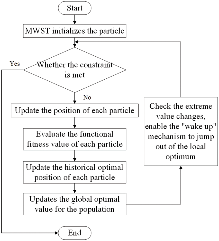
Figure 1: Flow chart of SAPSO algorithm

3.1 SAPSO Initialization Particle Structure Construction

The MWST generates the initial undirected graph by calculating MI. The construction principle is as follows: if the variable X may have three undirected edges X−Y,X−W,X−V. And I(X;Y)>I(X;W),I(X;Y)>I(X;V). In the MWST only reserved I(X;Y). According to this principle, all nodes are traversed in turn to create the largest MWST. It can be seen that the structure obtained from the largest MWST is an undirected graph. Because of the harsh conditions for generating edges, a node only retains one edge, so it is impossible to generate a ring structure after orientation. Therefore, in the absence of expert experience in node sequences. We adopt a randomly oriented way to generate a finite number of directed acyclic network structures with different node sequences.

Since the spanning tree has a small number of connected edges and a single choice of edges. As the number of nodes increases, the complexity of the network structure increases. Although the obtained network structure is non-looping, it is too simple. This makes the initialized particle diversity insufficient, and the initial particles need to be further increased and optimized, and expanded. To avoid producing too many useless directed edges, which have a negative impact on the subsequent algorithm. We use MI to solve this problem. Firstly, the dependence degree between each node and other nodes is calculated. The calculated MI results are sorted to obtain the corresponding Maximum Mutual Information (MMI). Then set the dynamic adjustment factor a=a+0.1R,R=1,2… to make the adjustment factor α gradually increase. In this way, the strong dependence relationship between node pairs is identified and the subsequently directed edges are constrained. When MI(xi,xj)>αMMI(xi)and MI(xi,xj)>αMMI(xj), we default that there is a strong dependency between the pair of nodes, which will generate connected edges. Otherwise, there are no connected edges. When α increases, the constraint conditions become more stringent. In this case, the number of node pairs satisfying the connection edge condition is reduced, and the generated initialization particle structure is relatively simple. On the contrary, when α decreases, the constraint conditions gradually become looser. The dependency requirements of node pairs are reduced. The number of node pairs that meet the condition of connecting edges increases, and the generated initial particle structure is relatively complicated. Assuming we have a directed acyclic network structure with P different node sequences. We can get R undirected edge addition combinations with different constraints by changing the regulation factor α R times. Then, P types of node sequences are generated by random orientation and a new edge-free orientation is added. Finally, check the acyclic and connectivity of the initial network structure. The overall process is shown in Fig. 2.

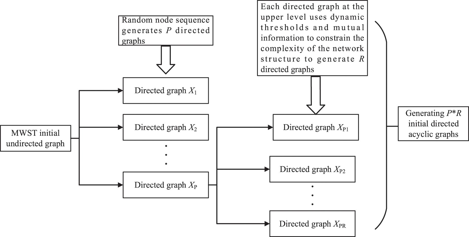
Figure 2: SAPSO generates initial particles

Definition: Two directed acyclic graphs DAG1 and DAG2 with the same node set are equivalent, if and only if:

(1)   DAG1 and DAG2 have the same skeleton;

(2)   DAG1 and DAG2 have the same V structure.

Since our initial PSO is based on the same spanning tree, even if the directivity of the edges is different, it is still easy to produce an equivalent class structure.

Since the initial PSO particles we obtained are based on the same spanning tree, it is easy to produce an equivalent class structure even if the directivity of the edges is different. To ensure the differences and effectiveness of each particle, the initial particle needs to be transformed once. Select the same structure with the same score to perform edges and subtraction, and finally get the final initial particles.

The pseudo-code at this stage is as follows:

Therefore, the initial network structure with some differences and high scores is obtained. Initialization dramatically reduces the search space of the BN structure. This will help reduce the number of iterative searches for the PSO and shorten the structure learning time in the next step.

3.2 Custom Update Based on PSO

The BN structure encoding is usually represented by the adjacent matrix, so the update equation of the PSO cannot be used directly. There are generally two methods. The first method is to use the binary PSO algorithm. And the second one is to use the improved PSO algorithm to enable it to adapt to the adjacent matrix update of the BN structure. Since the binary PSO requires a normalization function, the update operation of the particle needs to be performed several times, which will cause the results to be inaccurate. Therefore, we choose the second method to redefine the particle position and velocity to update the method. The flowchart is shown in Fig. 3.

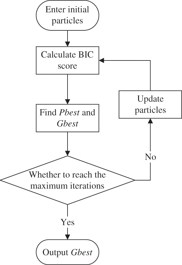
Figure 3: PSO custom update process

In BN structure learning, according to the characteristics of its search space, we define the adjacency matrix expressing DAG as the position of the particle Xt. Then we use the BIC score function as the fitness to determine the evaluation criteria. The higher the default fitness value, the better the particle. Thereby selecting the group extremum Gbest and the highest fitness value of each particle. Namely, the individual extremum Pbest. In Eq. (7), (Pbest−Xt) and (Gbest−Xt) are used as the update items of particles.

In BN structure learning, the expression form of position X is an adjacency matrix describing the network structure. Considering the rationality, it cannot directly correspond to the particle swarm update equation. The update process needs to be redefined. To facilitate the subsequent description, the update part is represented by an update.

The update process can adjust the position movement of the particles from both the direction and the step length. To get better feedback on the current status of the particle in the process of iteration. The positioning movement of the particles is divided into two steps, orientation, and fixed length. First, we use the fitness value to determine the current position of the particle and determine the direction of the particle’s movement.

updatedirection={V1(Move to Pbest)BICXit<BICPbestitV2(Move to Gbest)BICPbestit≤BICXit<BICGbesttV3(Nondirectional movement)BICXit≥BICGbestt(8)

Then we propose the complexity of particles as another index of particle renewal to determine the moving step size of particles. By comparing the number of edges in each network structure. We set the structure with a high fitness value as the target structure and calculate the complexity and compare it with the complexity of current particles.

update={Add side   complexityX<complexitytargetCut side   complexityX>complexitytargetReplace side    complexityX=complexitytarget(9)

Because the fitness of the target structure is better in the case of V1 and V2. Therefore, the complexity of the current particle structure should be closer to the target structure when the target structure is closer. When the complexity of the target structure is high, we choose to accelerate the current structure, that is, adding edge operations to make up for the shortcomings of the lack of complication of the current particle structure. Similarly, when the complexity of the target structure is lower, the current particles are reduced by edging operations. In the case of V3, the fitness of the current particle is better. Therefore, we replace the individual extreme value and the group extreme value with the current particle. Then move in a random direction with a fixed step. That is, the existing network structure is randomly added, cut, or reversed.

The entire location update operation can be expressed in two-dimensional coordinates. As shown in Fig. 4

Figure 4: Two-dimensional coordinates of PSO update factors

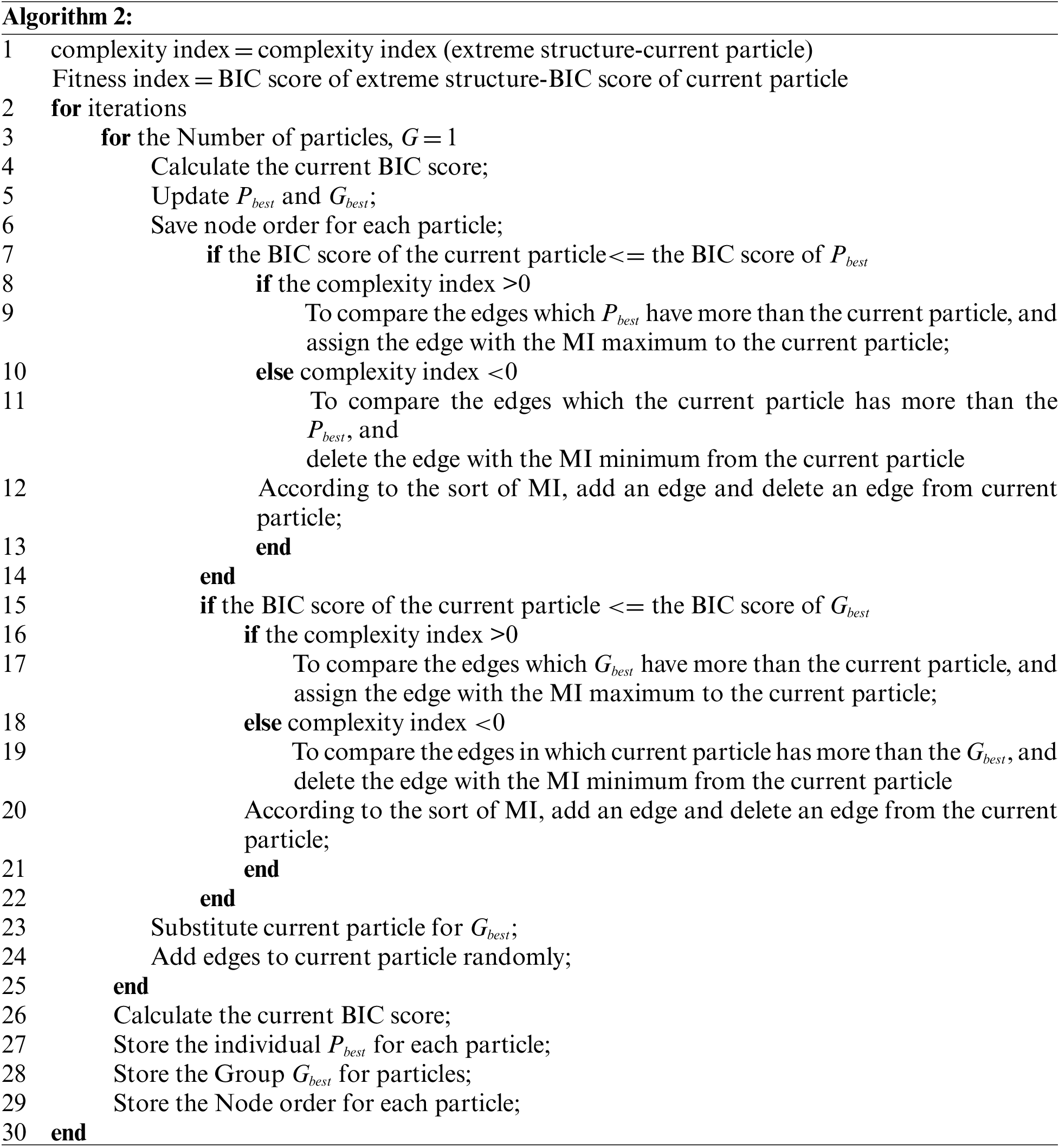
The complexity index is the difference between the number of directed edges of the target structure and the number of directed edges of the current particle structure. The fitness index is the difference between the fitness value of the target structure and the current particle. The fitness index determines whether the particle update method is a self-update or directional update and whether the current particle will replace the target particle. The complexity index determines whether the particle performs an edge addition operation or a subtraction operation. The pseudo code of the particle update process is shown as follows.

As the “group learning” part of the network structure, this algorithm can continuously find better solutions faster through iterative optimization and interactive learning of group information. However, it still has the shortcomings of too fast convergence and easy to fall into local optimum.

3.3 Breaking Out of the Local Optimal Particle “Self-Awakened” Mechanism

To further accelerate the learning efficiency of the algorithm while avoiding the learning process from falling into the local optimum. We set up a “self-awakened” mechanism. The specific process is shown in Fig. 5.

Figure 5: Particle “self-awakened” mechanism

T is used as the “premature factor” to identify whether the result has converged. When T≥3Gbest has passed more than three loop iterations and does not update. It means the result has converged. At this time, we force the deletion of the particle with the lowest BIC score and replace it with a new particle. There are two ways to generate new particles. One is to generate an adjacency matrix randomly. The other is to create new particles based on existing information. Because of the current mechanism requirements, it is necessary to add the best possible particles. Therefore, the best way is to make fine-tune based on the extremum of the group as a new particle to join the iterative optimization process. We learn from the update method of the mountain climbing algorithm, reverse the edge or randomly add the edge to Gbest. Then as the “self-awakened” particle replaces the particle with the lowest score before entering the loop. The specific update mechanism is shown in Eq. (10):

{Gbest+edge     rand<0.5Reverse edge     rand≥0.5(10)

Through the “self-awakened” mechanism, we can not only make the particles jump out of the local optimum but also update the node sequence, reducing the reverse edge caused by the misleading of the node sequence.

4  Experimental Results and Discussion

4.1 Experimental Preparation

In this section, to verify the performance of the algorithm. We chose the common standard datasets AISA network [30] and ALARM network [31] to complete the experiment. AISA network is a medical example that reflects respiratory diseases. State whether the patient has tuberculosis, lung cancer, or bronchitis associated with the chest clinic. Each variable can take two discrete states. The ALARM network has 37 nodes. It is a medical diagnostic system for patient monitoring. According to the standard network structure, the BNT toolbox is first used to generate datasets with sample sizes of 1000 and 5000 according to the standard probability table. Then the algorithm in this paper is used to learn the structure of the generated data. Meanwhile, the learning results were compared with improvement on the K2 algorithm via Markov blanket (IK2VMB) [32], max-min hill climbing (MMHC) [33], Bayesian network construction algorithm using PSO (BNC-PSO) [24], and BPSO [34] to verify the effectiveness of our algorithm.

We used four evaluation indicators:

(1)   The final average BIC score (ABB). This index reflects the actual accuracy of the algorithm.

(2)   The average algorithm running time (ART). This index reflects the running efficiency of the algorithm.

(3)   The average number of iterations of the best individual (AGB). This index reflects the algorithm’s complexity.

(4)   The average Hamming distance between the optimal individual and the correct BN structure (AHD). Hamming distance is defined as the sum of lost edges, redundant edges, and reverse edges compared to the original network. This index reflects the accuracy of the algorithm.

The experimental platform of this paper is a personal computer with IntelCorei7-5300U, 2.30 GHz, 8 GB RAM, and Windows 10 64-bit operator system. The programs were compiled with MATLAB software under the R2014a version, and the BIC score was used as the final standard score for determining structural fitness. Each experiment was repeated 60 times and the average value was calculated.

4.2 Comparison between SAPSO and Other Algorithms

In this section, we make an experimental comparison with BPSO, BNC-PSO, MMHC, and IK2vMB respectively. We set the population size to 100 and the number of iterations to 500. Independent repeated experiment 60 times to obtain the average. Table 1 shows the four datasets used in the experiment.

Table 2 compares the average time, BIC score value, average Hamming distance, average convergence generation, and BIC score of the initialized optimal structure for the four structure learning methods to train two network structures under different datasets. It can be seen that in the AISA network, the method in this paper is significantly better than the BNC-PSO, BPSO, MMHC, and IK2vMB algorithms in the accuracy of the learning structure, that is, the average error edge number and time.

Table 2 compares the experimental results of four structural learning algorithms in different datasets. Since MMHC and IK2vMB are not iterative algorithms, the average running time and convergence times are not counted. It can be seen from the table that in the AISA network, our algorithm is better than other algorithms in terms of learning accuracy and learning time. And with the increase of the dataset, the accuracy of the algorithm is constantly improving. Similarly, in the ALARM network, although the network structure becomes more complicated, the algorithm in this paper can still obtain the global optimal solution in a short time. It can complete the algorithm operations in the shortest time.

4.3 Performance Analysis of SAPSO

To better analyze the efficiency and performance of the algorithm, we compared the statistics of the previous section. As shown in Fig. 6.

Figure 6: The group’s extreme BIC score during the learning process of the 1000 dataset structure of the AISA network

The figure shows the relationship between the number of iterations and BIC scores in the AISA network in 1000 sets of datasets. It can be seen from the figure that the algorithm of this article can obtain the best BIC score value. Although the BPSO algorithm can converge as soon as possible, the algorithm’s accuracy is poor. The BPSO algorithm converges faster is that the BPSO algorithm is a global random search algorithm. The algorithm is randomly enhanced with the iterative operation, so the convergence speed is faster. However, because of its lack of local detection, it is more likely to fall into local optimal and lead to the rapid convergence of the algorithm. The algorithm we proposed is that the algorithm can quickly obtain the initial excellent initial planting group in the early stage of the search. And adding the self-awakened mechanism during the search stage, which allows the algorithm to jump out quickly after the local optimal is fell, and has obtained a globally optimal solution.

Fig. 7 shows the relationship between the number of iterations and the BIC scoring function of the 5000 sets of datasets of the Alarm network. Like the AISA network, this article algorithm can obtain the optimal network structure, but the advantages of BIC scores compared to other algorithms could be clearer. This is because as the complexity of the network structure increases, the algorithm advantage gradually weakens. Although the BIC score results are similar, the algorithm of this article is still better than other algorithms in Hamming distance and time efficiency.

Figure 7: The group’s extreme BIC score during the learning process of the 5000 dataset structure of the ALARM network

To further explain the role of the self-awakened mechanism, we choose a specific iteration process of an AISA network, as shown in Fig. 8. The algorithm obtained a local pole value in the early stage, but after a while, the algorithm eventually jumped out of the local pole value and obtained the global extreme value. This can verify the effectiveness of the algorithm in this article.

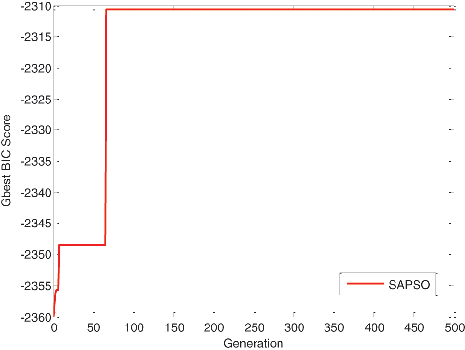
Figure 8: A study of the AISA network structure

5  Conclusion

This paper constructs a hybrid structure learning method based on the heuristic swarm intelligence algorithm PSO and MWST. First, an undirected graph is constructed through MWST, and then new directed edges are added to increase the diversity of initial particles through random orientation and MI constraint edge generation conditions. Form multiple connected directed acyclic graphs as the initial particles of PSO, and then use the idea of PSO to reconstruct the particle update process, with fitness and complexity as the conditions for judging the quality of particles, by adding edges, subtracting edges, and reversing edge. Finally, add a “ self-awakened “ mechanism in the PSO optimization process to constantly monitor the updated dynamics of the particle’s optimal solution, to survive the fittest, and replace the “inferior” particles with new particles in time to avoid premature convergence and local optimization. Experiments have proved that the initialization process of the particles makes the quality of the initial particles better and speeds up the optimization velocity of the particles; the reconstruction of the PSO optimization method allows the BN structure learning to be reasonably combined with the particle update so that the accuracy of the learning results higher; the “self-awakened” mechanism can effectively avoid the algorithm from prematurely converging into a local optimum. Compared with the experiments of other algorithms, the method in this paper can achieve shorter learning times, higher accuracy, and more efficiency. It can be further applied to complex network structures and to solve practical problems.

Although the algorithm proposed by us solves the learning problem of BN structure to a certain extent, the algorithm itself is affected by the scoring function, and multiple structures correspond to the same scoring result. Therefore, over-reliance on the scoring function has an impact on the final accurate learning of the structure. And selecting individual parameters in the PSO algorithm is not necessarily the optimal result. The following research work can improve the scoring function and study how to set the parameters of the PSO algorithm more reasonably, which can further reduce the algorithm complexity and improve the operation efficiency of the algorithm.

Acknowledgement: The authors wish to acknowledge Dr. Jingguo Dai and Professor Yani Cui for their help in interpreting the significance of the methodology of this study.

Funding Statement: This work was funded by the National Natural Science Foundation of China (62262016), in part by the Hainan Provincial Natural Science Foundation Innovation Research Team Project (620CXTD434), in part by the High-Level Talent Project Hainan Natural Science Foundation (620RC557), and in part by the Hainan Provincial Key R&D Plan (ZDYF2021GXJS199).

Author Contributions: The authors confirm contribution to the paper as follows: study conception and design: Kun Liu, Peiran Li; data collection: Kun Liu, Uzair Aslam Bhatti; methodology: Yu Zhang, Xianyu Wang; analysis and interpretation of results: Kun Liu, Peiran Li, Yu Zhang, Jia Ren; draft manuscript preparation: Kun Liu, Peiran Li; writing-review & editing: Kun Liu, Yu Zhang; funding: Jia Ren; supervision: Yu Zhang, Jia Ren; resources: Xianyu Wang, Uzair Aslam Bhatti. All authors reviewed the results and approved the final version of the manuscript.

Availability of Data and Materials: Data available on request from the authors. The data that support the findings of this study are available from the corresponding author Yu Zhang, upon reasonable request.

Conflicts of Interest: The authors declare that they have no conflicts of interest to report regarding the present study.

References

1. J. Dai, J. Ren, W. Du, V. Shikhin and J. Ma, “An improved evolutionary approach-based hybrid algorithm for Bayesian network structure learning in dynamic constrained search space,” Neural Computing and Applications, vol. 32, no. 5, pp. 1413–1434, 2020. [Google Scholar]

2. N. K. Kitson, A. C. Constantinou, Z. Guo, Y. Liu and K. Chobtham, “A survey of Bayesian network structure learning,” Artificial Intelligence Review, vol. 2023, pp. 1–94, 2023. [Google Scholar]

3. U. A. Bhatti, H. Tang, G. Wu, S. Marjan and A. Hussain, “Deep learning with graph convolutional networks: An overview and latest applications in computational intelligence,” International Journal of Intelligent Systems, vol. 2023, pp. 8342104, 2023. [Google Scholar]

4. M. H. M. Yusof, A. M. Zin and N. S. M. Satar, “Behavioral intrusion prediction model on Bayesian network over healthcare infrastructure,” Computers, Materials & Continua, vol. 72, no. 2, pp. 2445–2466, 2022. [Google Scholar]

5. Y. Zhou, X. Li and K. F. Yuen, “Holistic risk assessment of container shipping service based on Bayesian network modelling,” Reliability Engineering & System Safety, vol. 220, pp. 108305, 2022. [Google Scholar]

6. P. Chen, Z. Zhang, Y. Huang, L. Dai and H. Hu, “Risk assessment of marine accidents with fuzzy Bayesian networks and causal analysis,” Ocean & Coastal Management, vol. 228, pp. 106323, 2022. [Google Scholar]

7. C. Wang and K. Chen, “Analysis of network information retrieval method based on metadata ontology,” International Journal of Antennas & Propagation, vol. 2022, pp. 1–11, 2022. [Google Scholar]

8. J. Lessan, L. Fu and C. Wen, “A hybrid Bayesian network model for predicting delays in train operations,” Computers & Industrial Engineering, vol. 127, pp. 1214–1222, 2019. [Google Scholar]

9. J. Shen, F. Liu, M. Xu, L. Fu, Z. Dong et al., “Decision support analysis for risk identification and control of patients affected by COVID-19 based on Bayesian networks,” Expert Systems with Applications, vol. 196, pp. 116547, 2022. [Google Scholar]

10. R. Moradi, S. Cofre-Martel, E. L. Droguett, M. Modarres and K. M. Groth, “Integration of deep learning and Bayesian networks for condition and operation risk monitoring of complex engineering systems,” Reliability Engineering & System Safety, vol. 222, pp. 108433, 2022. [Google Scholar]

11. C. Zhang, M. Jamshidi, C. C. Chang, X. Liang, Z. Chen et al., “Concrete crack quantification using voxel-based reconstruction and Bayesian data fusion,” IEEE Transactions on Industrial Informatics, vol. 18,no. 11, pp. 7512–7524, 2022. [Google Scholar]

12. A. Siahkoohi, G. Rizzuti and F. J. Herrmann, “Deep Bayesian inference for seismic imaging with tasks,” Geophysics, vol. 87, no. 5, pp. S281–S302, 2022. [Google Scholar]

13. A. Srivastava, S. P. Chockalingam and S. Aluru, “A parallel framework for constraint-based Bayesian network learning via markov blanket discovery,” IEEE Transactions on Parallel and Distributed Systems, vol. 2023, pp. 1–17, 2023. [Google Scholar]

14. C. Contaldi, F. Vafaee and P. C. Nelson, “Bayesian network hybrid learning using an elite-guided genetic algorithm,” Artificial Intelligence Review, vol. 52, no. 1, pp. 245–272, 2019. [Google Scholar]

15. K. Tsirlis, V. Lagani, S. Triantafillou and I. Tsamardinos, “On scoring maximal ancestral graphs with the max–min hill climbing algorithm,” International Journal of Approximate Reasoning, vol. 102, pp. 74–85, 2018. [Google Scholar]

16. W. Song, L. Qiu, J. Qing, W. Zhi, Z. Zha et al., “Using Bayesian network model with MMHC algorithm to detect risk factors for stroke,” Mathematical Biosciences and Engineering, vol. 19, no. 12, pp. 13660–13674, 2022. [Google Scholar] [PubMed]

17. X. Zhang, Y. Xue, X. Lu and S. Jia, “Differential-evolution-based coevolution ant colony optimization algorithm for Bayesian network structure learning,” Algorithms, vol. 11, no. 11, pp. 188, 2018. [Google Scholar]

18. H. Q. Awla, S. W. Kareem and A. S. Mohammed, “Bayesian network structure discovery using antlion optimization algorithm,” International Journal of Systematic Innovation, vol. 7, no. 1, pp. 46–65, 2022. [Google Scholar]

19. B. Sun, Y. Zhou, J. Wang and W. Zhang, “A new PC-PSO algorithm for Bayesian network structure learning with structure priors,” Expert Systems with Applications, vol. 184, pp. 115237, 2021. [Google Scholar]

20. G. Li, L. Xing and Y. Chen, “A new BN structure learning mechanism based on decomposability of scoring functions,” in Bio-Inspired Computing–Theories and Applications, Hefei, China, pp. 212–224, 2015. [Google Scholar]

21. X. Liu and X. Liu, “Structure learning of Bayesian networks by continuous particle swarm optimization algorithms,” Journal of Statistical Computation and Simulation, vol. 88, no. 8, pp. 1528–1556, 2018. [Google Scholar]

22. T. Wang and J. Yang, “A heuristic method for learning Bayesian networks using discrete particle swarm optimization,” Knowledge and Information Systems, vol. 24, pp. 269–281, 2010. [Google Scholar]

23. J. Wang and S. Liu, “A novel discrete particle swarm optimization algorithm for solving Bayesian network structures learning problem,” International Journal of Computer Mathematics, vol. 96, no. 12, pp. 2423–2440, 2019. [Google Scholar]

24. S. Gheisari and M. R. Meybodi, “BNC-PSO: Structure learning of Bayesian networks by particle swarm optimization,” Information Sciences, vol. 348, pp. 272–289, 2016. [Google Scholar]

25. X. L. Li, “A particle swarm optimization and immune theory-based algorithm for structure learning of Bayesian networks,” International Journal of Database Theory and Application, vol. 3, no. 2, pp. 61–69, 2010. [Google Scholar]

26. L. E. Sucar and L. E. Sucar, “Bayesian networks: Learning,” Probabilistic Graphical Models: Principles and Applications, vol. 2021, pp. 153–179, 2021. [Google Scholar]

27. X. Qi, X. Fan, H. Wang, L. Lin and Y. Gao, “Mutual-information-inspired heuristics for constraint-based causal structure learning,” Information Sciences, vol. 560, pp. 152–167, 2021. [Google Scholar]

28. H. Guo and H. Li, “A decomposition structure learning algorithm in Bayesian network based on a two-stage combination method,” Complex & Intelligent Systems, vol. 2022, pp. 1–15, 2022. [Google Scholar]

29. A. G. Gad, “Particle swarm optimization algorithm and its applications: A systematic review,” Archives of Computational Methods in Engineering, vol. 29, no. 5, pp. 2531–2561, 2022. [Google Scholar]

30. S. L. Lauritzen and D. J. Spiegelhalter, “Local computations with probabilities on graphical structures and their application to expert systems,” Journal of the Royal Statistical Society: Series B (Methodological), vol. 50, no. 2, pp. 157–194, 1988. [Google Scholar]

31. I. A. Beinlich, H. J. Suermondt, R. M. Chavez and G. F. Cooper, “The ALARM monitoring system: A case study with two probabilistic inference techniques for belief networks,” in AIME 89: Second European Conf. on Artificial Intelligence in Medicine, London, England, pp. 247–256, 1989. [Google Scholar]

32. J. Jiang, J. Wang, H. Yu and H. Xu, “Poison identification based on Bayesian network: A novel improvement on K2 algorithm via Markov blanket,” in Advances in Swarm Intelligence: 4th Int. Conf., ICSI 2013, Harbin, China, pp. 173–182, 2013. [Google Scholar]

33. I. Tsamardinos, L. E. Brown and C. F. Aliferis, “The max-min hill-climbing Bayesian network structure learning algorithm,” Machine Learning, vol. 65, no. 1, pp. 31–78, 2006. [Google Scholar]

34. X. Chen, J. Qiu and G. Liu, “Optimal test selection based on hybrid BPSO and GA,” Chinese Journal of Scientific Instrument, vol. 30, no. 8, pp. 1674–1680, 2009. [Google Scholar]