Speech Recognition via CTC-CNN Model

1  Introduction

Speech is a linguistic term coined by the Swiss linguist Saussure; it is a concept that is opposite to language. Speech activity is mainly controlled by the individual’s free will; it has characteristics of personal pronunciation, word use, expression and emotion, etc. In contrast, language is a social part of speech activity, not dominated by individual will, but shared by members of society, and arises as a social psychological phenomenon. Speech activity, as defined by the linguist Saussure, is used to collectively describe the phenomenon of human speech. Human language is a natural and effective means of communication, and it is required at most levels of life to communicate with and be understood by others. Verbal communication is taken for granted by most people. In contrast, if an individual’s pronunciation or expression makes it difficult for others to even understand what they are saying, it is highly inconvenient and frustrating.

Millions of people worldwide are unable to pronounce correctly and fluently due to disorders, such as strokes, amyotrophic lateral sclerosis (ALS), cerebral palsy, traumatic brain injury, or Parkinson’s disease. In response to this problem, we propose an end-to-end neural network architecture, as the connectionist temporal classification-convolutional neural network (CTC-CNN) to help these people communicate normally. Deep learning is mainly used in visual recognition, speech recognition, natural language processing, biomedicine and other fields, and has achieved good results. This research will use deep learning technology to develop a deep intelligent speech processing system, effectively integrating signal processing, acoustic processing, language processing and deep learning. We will research and develop intelligent multi-channel speech processing and speech separation, optimize speech recognition, speech translation, speech emotion recognition and innovation. In the front-end processing, we propose a multi-channel speech enhancement algorithm based on deep learning, and this algorithm integrates beamforming technology and deep neural network. In terms of speech separation, we propose a single-channel speech separation (SCSS) model based on GP regression. The source of the estimate is measured by the predicted mean of the Gaussian Process (GP) regression model, and the hyper-parameter learning process is performed by using a nonlinear conjugate gradient algorithm. We propose Hierarchical Extreme Learning Machine (HELM) for audiovisual speech enhancement as an alternative model for speech enhancement tasks. To enhance speech recognition, the use of a novel graph regularization-based method is proposed to enhance speech features by preserving the intrinsic diversity structure of the amplitude modulation spectrum and excluding irrelevant ones. In machine translation, bidirectional translation between English and Chinese is provided. The speech emotion recognition system uses a multi-feature extraction network based on deep learning and a self-developed recurrent neural network. To understand the semantics of dialogue, language understanding techniques for dialogue systems are developed. This study is developed with the deep learning speech recognition system of this study. Through intelligent speech recognition technology, the speech learning robot allows users to practice pronunciation and pronunciation in a speech environment. Robustness technology mitigates the adverse effects of environmental distortions to maintain acceptable performance levels for automatic speech recognition systems. Deep learning is widely used today because of its powerful learning ability, it can be trained through large-scale data sets, and autonomously extract and learn complex features and models from it. Deep learning uses a multi-layer neural network model that allows the exclusion of layers. Extract an abstract feature representation of the data. Through the combination of multiple hidden layers, the model can learn higher-level and abstract special performance, thereby improving the performance of the model, and at the same time, it can handle large data statistics and efficiently use these large model data to learn more from it. Accurate and generalized models, and can be learned and trained in an end-to-end manner, that is, from the initial input data, the final result is directly output, without the need to manually design complex special processes. This simplifies the development process of the machine learning system and improves the efficiency and accuracy of the model.

However, in the field of speech recognition, the performance of the acoustic model directly affects the accuracy and stability of the final speech recognition system, requiring detailed consideration of its establishment, optimization and efficiency [1]. The experiments in this study adopt CTC-CNN to train the acoustic model, and CTC-CNN shows better performance than the Gaussian Mixture Model-Hidden Markov Model (GMM-HMM) acoustic model commonly used earlier. We use state-of-the-art techniques to validate our method. Experimental results show that the effect is remarkable. Fig. 1 illustrates the historical evolution of automatic speech recognition (ASR).

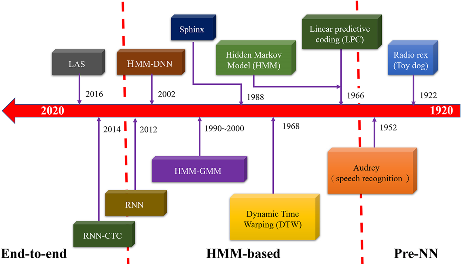
Figure 1: Historical development of automatic speech recognition

In the traditional speech recognition system, the mismatch between the model training environment and the test environment (mismatch) is the primary problem that causes the recognition rate to decline. On this issue, many solutions have been proposed in the past literature, such as introducing model parameters at the speech model end. Robust CTC-CNN Model prediction classification rules established by uncertainty, or adjustment methods to adjust the model to the test environment, such as maximum posterior probability (MAP) adjustment and linear regression adjustment, and even further consider the discrimination of speech models the minimum classification error linear regression (MCELR) adaptation and other methods. Among them, the CTC-CNN Model prediction classification method is to properly introduce the uncertainty of the model parameters into the decision-making rule to achieve the robustness of the decision-making method, and the parameter uncertainty reflects the variability of the noise environment and acoustics. It can be represented by the prior probability, and the traditional CTC-CNN Model learning provides a mechanism for estimating and updating parameter prior information. In order to take into account the robustness and discriminability of the decision rule, this study proposes the discriminative training and updating of the acoustic model and its prior probability model under the CTC-CNN Model predictive classification framework. We use the discriminative criterion of minimum classification error (MCE) to Estimate the hyper-parameter of the model parameters, and propose two update methods, one is to directly update the pre-statistics for the hidden Markov model mean vector parameters; the other is to consider the linear regression adjustment, for the regression matrix. The prior information is updated under the minimum classification error criterion. In the evaluation experiment based on the environmental noise speech database, it is found that using the updated prior probability can improve the discrimination of the CTC-CNN Model prediction classification, and achieve the purpose of improving the performance of robust speech recognition.

In this field of research, many scholars have proposed different methods to solve the problem of mismatch, which we roughly divide into three categories: signal space, feature parameter space, and model parameter space. In the first method, the method of speech enhancement is mainly used. The idea is to reduce the noise part of the signal affected by the environment through signal processing to obtain an approximately clean signal; the second method. The first method is similar to the processing concept of the signal space. It is hoped to restore the characteristics of the characteristic parameters in the original environment and perform compensation of the characteristic parameters; the last method is to process the model parameters that have been trained. It is subdivided into two types: one is to use a small amount of corpus obtained from the new environment to adapt the original model parameters to a method close to the new environment; the other is to consider its uncertainty in the model parameters to reduce The impact caused by model variation, and then achieve the mechanism of robust decision-making. In addition, during model training, parameters or distributions between different models often face confusion, resulting in increased classification errors. Therefore, the consideration of discriminability has also been proposed by scholars to be introduced into the training process of the model in order to achieve a clearer result.

In this study, based on considering the uncertainty of the parameters, it is hoped that the uncertainty of its parameters can be updated under the consideration of the discriminative classification method, to further achieve robust decision-making with discriminative prior probability law. In this study, the prior probability learning that considers uncertainty and is discriminative is also implemented in the adjustment of model parameters, which is divided into the direct adjustment of model parameters and indirect adjustment of model parameters. In the continuous digital corpus dominated by environmental noise, the improvement of recognition performance can be achieved. This study uses Google’s public training data set—Speech Commands Dataset for analysis and deep learning model training, which contains 30 different word audio files, and each word, has about 2300∼2400 original wav audio files. Based on this data set, data preprocessing (including analysis and conversion of sound waves, cutting of training and test data, etc.) will be performed, and Keras and various packages will be used in the Python environment to construct a convolutional neural network model and Long-term short-term memory model for image recognition training on converted data.

2  Literature Survey

In this era of technological progress, speech recognition technology has been applied in numerous fields, most of which are mainly based on intelligent electronics and driving navigation products. In addition to helping people troubled by language barriers and unable to communicate normally due to disease or various disorders, this research has the potential to bring more convenience to their lives. In the experimental architecture, this model considers linguistics, speech recognition applications, and deep learning techniques. This approach provides assists to individuals with speech recognition and language impairments, it is necessary to understand the basic linguistic theory. Because language belongs to human spontaneous speech, it contains numerous irregular variables, such as personal pronunciation, words, expressions, and various factors that lead to a certain degree of complexity in establishing the acoustic model to ensure that it meets the requirements as much as possible. Deep learning serves to improve the efficiency and accuracy of the acoustic model performance.

In view of the fact that the application of artificial intelligence in various fields has increased significantly in recent years, understanding the basic concepts of deep learning and the implementation of programs has become an important learning goal. According to the obtained original data, we can further analyze and understand the characteristics of the data, and then it is an important issue to select and use various neural networks to construct models. Among the application fields of deep learning, the most important ones are image recognition and natural language processing. Therefore, this research intends to carry out a simple program implementation for the latter field, using Convolutional Neural Network (CNN) and Long Short-Term Memory (LSTM) to implement a simple speech recognition model, hoping to recognize simple words, and also through parameter tuning design and experiments, in order to develop a high-accuracy identification model.

Speech recognition is a technology in which a computer converts the speaker’s pronunciation into text by comparing the acoustic features. In the 1980s, research in this field was initiated by the laboratory of the Massachusetts Institute of Technology, but due to the low recognition rate, it has not been able to be applied to commercial purposes. It was not until 2012 that scientists replaced the traditional Gaussian distribution calculation with the calculation method of DNN, which greatly improved the recognition rate, that it gradually attracted the attention and attention of large international companies. The main process of using a deep network to realize automatic speech recognition is: to input speech fragments (Spectrogram, MFCCs, …, etc.), convert the original language into acoustic features, and then pass through the judgment and probability distribution of the neural network, and finally output the corresponding text content.

The two neural networks used in this study are the LSTM of the CNN and the Recurrent Neural Networks (RNN). CNN is a convolutional neural network consisting of a convolutional layer, a fully connected layer, and a pooling layer. With the operation of the backpropagation algorithm, it can use the two-dimensional structure of the input data to extract features and properly converge and learn. Speech recognition has excellent performance. RNN is a neural network with active data memory called LSTM, which can be used for a series of data to guess what will happen next. Its output is not only consistent with the current input and network it is related to the weight of the road, and also related to the input of the previous network. It is often used to process time series data. Now it has been widely used in natural language understanding (such as speech-to-text, translation, and hand-written text generation), image and video recognition, and other fields.

2.1 Speech Recognition

In recent years, the use of speech recognition has been spreading widely across various fields, and it is no longer limited to intelligent electronics products, but gradually expanding to the healthcare industry and even to product sales and customer services. A good speech recognition system must allow organizations to customize and adapt the technology to their specific needs, ranging from nuances in language to speech to everything else. For example:

1. Language weighting: A discriminative weighted language model is proposed to better distinguish similar languages. Similar utterances or words are weighed to improve the accuracy [2].

2. Speaker markers: Speaker selection, taking turns, elaboration, and digression. After providing definitions of discourse markers, turns, floor control types/turn segments, topic units, and actions, a list of verbal and non-verbal discourse markers is specified and grouped into subcategories according to their semantic relationship [3].

3. Acoustic training: Building acoustic models from large databases has been shown to benefit the accuracy of speech recognition systems. Deep learning is employed to train these systems to adapt to various acoustic environments, such as speaker pronunciation, speech rate, pitch, etc., to cope with a variety of different situations.

4. Indecent content filtering: Filters are used to identify profanity words or nonsense particles, etc., and eliminate this type of speech [4].

2.1.1 Pattern Recognition

Current mainstream large-vocabulary speech recognition systems mostly use statistical pattern recognition technology. A typical speech recognition system based on the statistical pattern recognition method consists of the following basic modules:

1. Signal processing and feature extraction modules: The main work of this module is to extract sound features from the input signal and provide them with an acoustic model for processing. It also includes signal processing techniques to minimize the influence of environmental noise, channel, speaker, and other factors on the characteristics.

2. Acoustic model: Typical systems are mostly modeled based on first-order hidden Markov models.

3. Pronunciation dictionary: The pronunciation dictionary contains the vocabulary and pronunciations that can be handled by the system. The pronunciation dictionary provides the mapping between the acoustic model modeling unit and the language model modeling unit.

4. Language model: A statistical language model represents a probability distribution over a sequence of words, and a language model mainly provides the context to distinguish two words and phrases that have similar pronunciations but different meanings, as shown in the example in Fig. 2. This model is often used in numerous natural languages processing applications, such as speech recognition, machine translation, and part-of-speech tagging, etc. Because words and sentences are of any length in any combination, strings that have not appeared in the training process will appear. This further makes it difficult to estimate the probability of strings in the database.

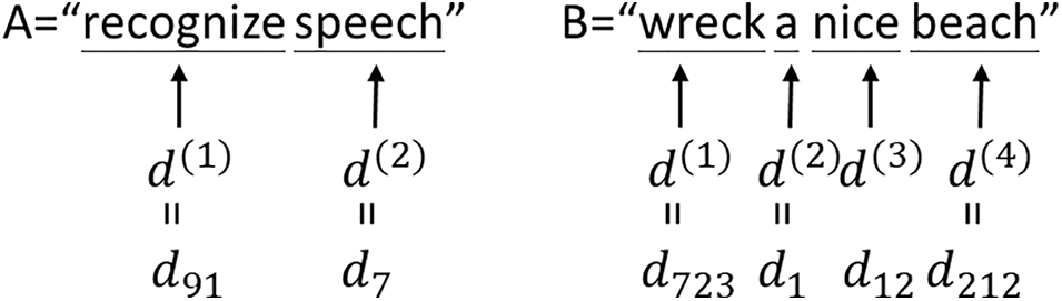
Figure 2: Two homonymous English strings

5. Decoder: The decoder is one of the core aspects of the speech recognition system. It mainly uses the input signal to find the word string that outputs the signal with the greatest probability according to acoustics, language models, and dictionaries.

Fig. 2 illustrates two homonymous English strings. In the language model, in addition to the pronunciation that affects the accuracy of speech recognition, punctuation is likewise an important reason that affects the recognition of the system. Therefore, we discuss several considerations when constructing a post-processing system: (1) Restoring the original requires a high-accuracy model of text punctuation and capitalization. The model must make quick inferences about interim results and catch up on instant captions. (2) Using several resources: Speech recognition is an AND operation-intensive technology, such that punctuation patterns do not need to be so computationally intensive. (3) Ability to handle text not listed in the vocabulary: sometimes, the system must add punctuation or capitalization to text that the model has not seen before.

2.1.2 Speech Recognition Algorithms

Speech recognition is considered one of the most complex fields in modern technology, as it involves linguistics, mathematics, and statistics. At present, the common speech recognition system is mainly composed of several technologies, such as: speech signal input, feature extraction, acoustic model establishment, feature vector, decoder, and result output. Speech recognition technology is evaluated based on its accuracy, word error rate (WER), and speed. A variety of factors affect the misspelling rate.

Here are some of the various algorithms and techniques that are currently most commonly used to recognize speech and convert it to text:

1. Natural Language Processing (NLP) belongs to the field of artificial intelligence, which focuses on language interaction between humans and machines through speech and text. Numerous mobile devices currently incorporate speech recognition into their systems to provide more assistance.

2. Hidden Markov Model (HMM) is used as a sequence model in speech recognition, assigning labels to each unit in the sequence, i.e., words, syllables, sentences, etc. These labels map between them and the input provided, such that it can determine the most appropriate sequence of labels.

3. N-grams is the simplest type of language model (LM) that assigns probabilities to sentences or phrases. An N-gram is a sequence of N words. For example: “How are you” is a ternary, and “I’m fine thank you” is a quaternary. Grammar and specific word sequence probabilities are used to enhance recognition and accuracy.

4. Neural networks are mainly used in deep learning algorithms. They learn the mapping function through supervised learning and adjust it according to the loss function during gradient descent.

5. Speaker Discrimination (SD) algorithms identify and separate utterances by speaker identity. This helps the system make better distinctions between individuals in a conversation [5].

2.2 Convolutional Neural Networks Applied in This Study

2.2.1 CTC-CNN Acoustic Model

In the speech recognition system, the acoustic model is an important underlying model, and its accuracy directly affects the performance of the entire system. When acoustic features remain unchanged, the performance of the speech recognition system is mainly improved by optimizing the acoustic model. Early speech recognition systems mainly employ the GMM-HMM acoustic model, which is a shallow model. Thus, it is difficult to accurately describe the state space distribution of features. Furthermore, the frame-by-frame training mode requires mandatory alignment of the training speech, which increases the difficulty of model training. With the development of deep learning, speech recognition systems began to use deep learning-based acoustic models and achieved remarkable results. The latest end-to-end speech recognition framework abandons the more restrictive model of HMM, and directly optimizes the likelihood of input and output sequences, which significantly simplifies the training process. Deep neural networks, loop neural networks, and convolutional neural networks achieved great results in the field of speech recognition with their advantages [6].

In this study, the convolutional neural network was mainly used to build the acoustic model combined with the connection sequence classification algorithm, which significantly improves the accuracy and performance of the speech recognition system. Based on the establishment of the baseline acoustic model, this research significantly reduces the error rate of the speech-to-pinyin sequence by continuously optimizing the acoustic model. As the output of the acoustic model, the choice of the modeling unit is also one of the factors affecting the performance of the acoustic model. When selecting a modeling unit, it is necessary to consider: (1) whether the modeling unit fully represents the context information, i.e., the accuracy of the modeling unit; (2) whether it can describe the acoustic features for generalizability; (3) whether there is sufficient language material that can satisfy the modeling unit for model training and trainability. When building the speech recognition system in this study, a non-complete end-to-end speech recognition framework is employed, i.e., the acoustic model uses the end-to-end recognition framework to convert speech into pinyin sequences, and then uses the language model to convert the pinyin sequences into text. In this study, a convolutional neural network is used to build the acoustic model, which is combined with the connectionist temporal classification (CTC) algorithm to realize the conversion of phonetic to pinyin sequences. Traditional classification methods face problems, such as unequal input and output lengths, and frame-by-frame training is required. CTC can directly map the input speech sequence into a string of text sequences, such that it can optimize the likelihood of the input and output sequences, which significantly simplifies the training process. The essence of the acoustic model based on CTC remains a sequence classification problem, meaning that the output of each node in the output layer of the neural network selects a generation path with the highest probability. Therefore, the input and output of CTC are often in a many-to-one relationship [7]. When the CTC-based acoustic model recognizes speech, the acoustic feature parameters are further extracted through the convolutional neural network, and then the posterior probability matrix is output through the fully connected network and the SoftMax layer. The maximum probability label of each node is thus used as the output sequence. Finally, the optimized output label sequence of the CTC decoding algorithm marks the recognition result. The schematic diagram of the CTC-CNN acoustic model is shown in Fig. 3 [8].

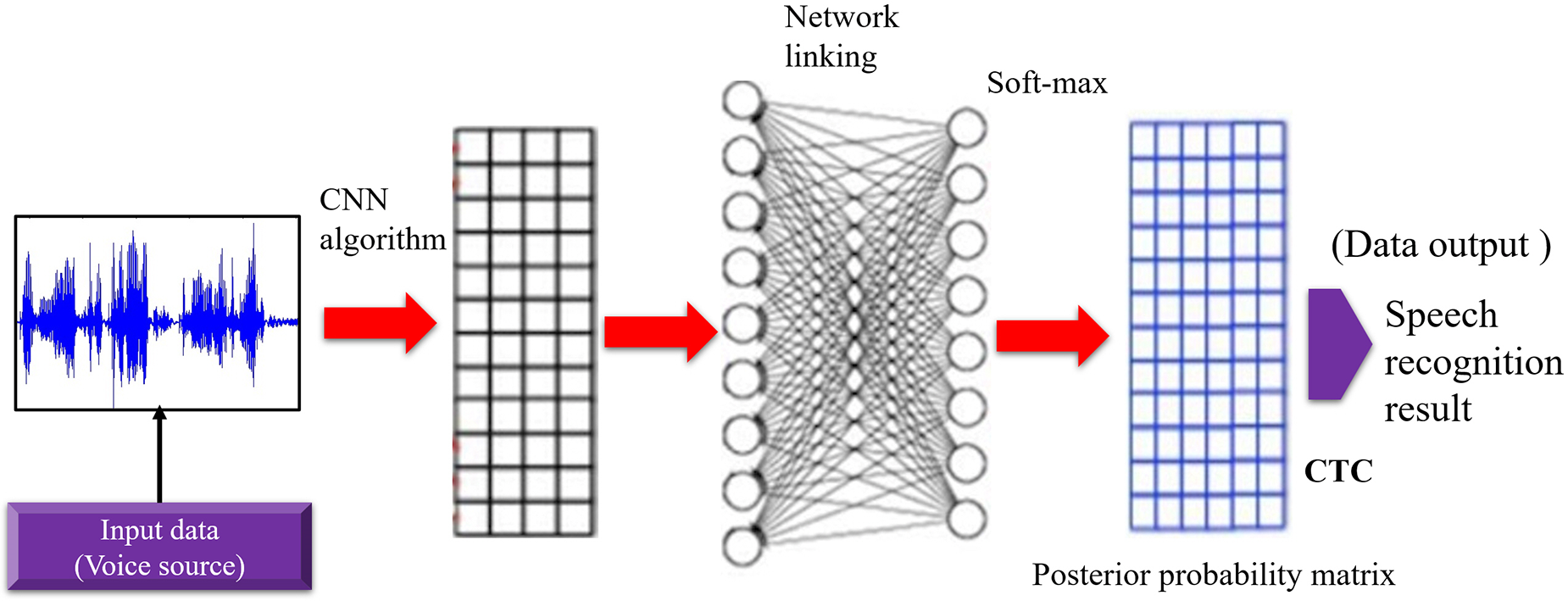
Figure 3: Schematic chart of CTC-CNN acoustic model

2.2.2 Core Idea of CTC

The core ideas of CTC mainly include the following parts:

(1) Expanding the output layer of CNN, adding a many-to-one spatial mapping between the output sequence and the recognition result (label sequence), and defining the CTC loss function on this basis.

(2) Drawing on the idea of the forward algorithm of HMM, the dynamic programming algorithm is used to effectively calculate the CTC loss function and its derivative, thus solving the problem of end-to-end training of CNN [9].

(3) Combined with the CTC decoding algorithm, the end-to-end prediction of sequence data is effectively realized [10].

Assuming that the speech signal is x, and the label sequence is l, the neural network obtains the probability distribution of the label sequence (l|x) during the training process. Therefore, after inputting the speech, the output sequence is selected with the highest probability, and after CTC decoding optimization, the final recognition result O(x) can be output, where the operation formula is shown in Eq. (1).

O(x)=argmaxP(l|x)(1)

Given a CNN acoustic model for CTC derivation training, we first assume that S is the training data set, X is the input space, Z is the target space (the set of labeled sequences), and L is defined as the sum of all output labels (modeling units). Set, CTC extends L to L′=L∪Blank. Under given conditions, the probability of outputting a label k at a time t can be expressed as Eq. (2).

ykt=P(Ot=k|x1,x2,…,xt)(2)

Assuming that under the condition of a given input sequence x, the output label probability is independent at the time t, and L′T is defined as the set of output sequences of length T composed of L′, then the conditional probability formula of a path π ∈ L′T is given by Eq. (3).

P(π|x)=∏t=1Tyπt t(3)

We define the mapping relationship B: L′T → L≤T from the path π to the label sequence l. Using this mapping relationship will keep only one consecutive and identical label in the output sequence contained in the path π, and remove the Blank label. Then, to calculate the probability of label sequence l ∈ L≤T, it is necessary to accumulate all path probabilities belonging to l, and the calculation formula is shown in Eq. (4).

P(l|x)=∑π∈B−1(l)P(π|x)(4)

The mapping of the path π to label sequence l is shown in Fig. 4.

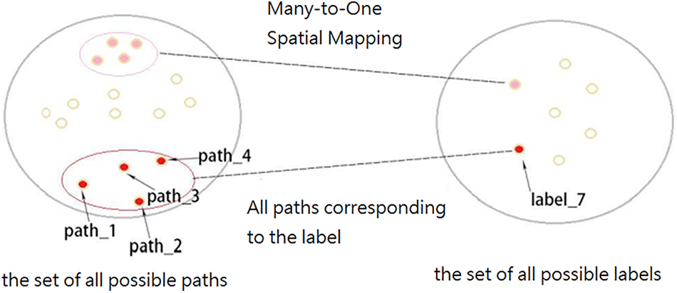
Figure 4: Mapping output to label sequence

Fig. 4 shows that the probability of label sequence label_7 is equal to the total probability of its entire path, that is, P (label_7) = P (path_1) + P (path_2) + P (path_3) + P (path_4). It is impractical to directly violently calculate (l|x), which will increase the training time of the model and occupy computing power. Borrowing the forward and backward algorithm in HMM effectively solves (l|x), and it is assumed that under the condition of a given input sequence x, the output label probability at the time t is independent, such the transition probability between states does not need to be considered. The derivation diagram of the forward and backward algorithm is shown in Fig. 5 [11].

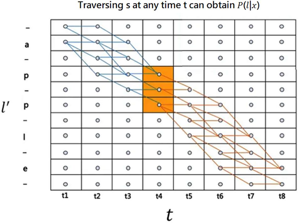
Figure 5: Derivation of forward and backward algorithm

The calculation of the forward-backward algorithm is as follows: For the input sequence x and the label sequence l with the time sequence length T, the extended label sequence is l′, and the length of the extended label sequence is |l′| = 2|l| + 1, defining the first t. The forward probability of outputting the extended label at the sth position at the moment is α(t,s), and the posterior probability calculation formula of the label sequence is shown in Eq. (5) [12].

P(l|x)=α(T, |l′|)+α(t, |l′|−1)(5)

Before calculating the forward probability, the parameters must be initialized first, and the Blank label is abbreviated as b, such that the calculation formula is Eq. (6).

α(1,1)=yb1; α(1,2)=yl2′1; α(1,s)=0(∀s>2)(6)

The recursive calculation formula of forward probability obtained by recursion is shown in Eq. (7).

α(t, s)={(α(t−1,s)+α(t−1,s−1))yls′ t if ls′ =b or ls−2′ =ls′  (α(t−1,s)+α(t−1,s−1)+α(t−1,s−2))yls′ t others(7)

The backward algorithm is similar to the forward algorithm. The backward probability of outputting the extended label at the sth position at the time t is defined as (t,), and the posterior probability calculation formula of the label sequence is shown in Eq. (8).

P(l|x)=β(1,1)+β(1,2)(8)

Before calculating the backward probability (t,), we initialize the parameters, as shown in Eq. (9).

β(T, |l′|)=yBT, β(T, |l′|−1)=yl|l′|−1′T, β(T, s)=0(∀s<|l′|−1)(9)

The recursive calculation formula of the backward probability obtained by recursion is shown in Eq. (10).

β(t, s)={(β(t+1,s)+β(t+1,s+1))yls′ t if ls′ =b or ls+2′ =ls′  (β(t+1,s)+β(t+1,s+1)+β(t+1,s+2))yls′ t others(10)

For any moment t, the posterior probability of the label sequence is calculated using the forward and backward probabilities, and the calculation formula is shown in Eq. (11).

P(l|x)=∑s=1|l′|α(t, s)β(t, s)yls′ t(11)

With the posterior probability calculation formula (l|x) of the label sequence, the training target can be optimized, and the parameters can be updated. The loss function of CTC is defined as the negative log probability of the label sequence on the training set S. Then, the loss function (x) output of each sample is given by Eq. (12).

L(x, l)=−lnP(l|x)(12)

The loss function LS of the entire training set is given by Eq. (13).

LS=−∑(x,l)∈S lnP(l|x)(13)

The loss function L takes the derivative of the network output parameter ykt, and its operation formula is shown in Eq. (14).

∂L∂ykt=− ∂∂yktln⁡P(l|x)=−1ln⁡P(l|x)∂∂ykt ln⁡P(l|x)(14)

The chain rule yields the partial derivative of the loss function to the network output ukt without the SoftMax layer. Because a character k may appear multiple times in a label sequence, a set is defined to represent the position where k appears: (l) = {s:ls = k}. It is obtained as Eq. (15).

−∂ln⁡P(l|x)∂ukt=ykt−1P(l|x)ykt∑s∈lab(l,k)α(t, s)β(t, s)(15)

The parameters of the neural network part are updated layer by layer and frame by frame according to the back-propagation algorithm. When CTC decodes the output, the output sequence must be optimized to obtain the final label sequence. This study adopts the best path decoding algorithm, assuming that the probability maximum path π and the probability maximum label l∗ have a one-to-one correspondence, meaning that the many-to-one mapping B has degenerated into a one-to-one mapping relationship, and the algorithm accepts each frame. The label sequence corresponding to the output sequence generated by the maximum probability label is used as the final recognition result. First, we must calculate the maximum probability path π∗ output by the network, and the operation formula is shown in Eq. (16) [13].

π∗=argmax P(π|x)(16)

Then, we calculate the label sequence output by the network, and define l∗ = (π∗). The formula l∗ is given by Eq. (17).

l∗=B(argmaxπ P(π|x))(17)

The recognition result of the final acoustic model is given by Eq. (17). In essence, the acoustic model of CTC can be directly output to Chinese characters end-to-end. Due to the limitation of the training corpus and the complexity of the model, the output of the acoustic model in this study is Pinyin; the final result of speech recognition is obtained by inputting the pinyin sequence into the language model [14–16].

2.2.3 Construction and Training of Baseline Acoustic Model

In the convolutional neural network, the structure of the convolutional and pooling layers indicate that the input features with slight deformation and displacement are accurately recognized. This translation invariance characteristic is beneficial to the recognition of spectrogram features. The training mode of parallel computing of the convolutional neural network effectively shortens the training time and utilizes the powerful parallel processing capability of Graphics Processing Unit (GPU). CTC illustrates the optimization of the loss function of the neural network and the optimization of the output sequence. Therefore, this study proposes a CTC-CNN acoustic model based on CNN combined with the CTC algorithm. The overall structure of the CTC-CNN acoustic model is shown in Fig. 6 [17,18].

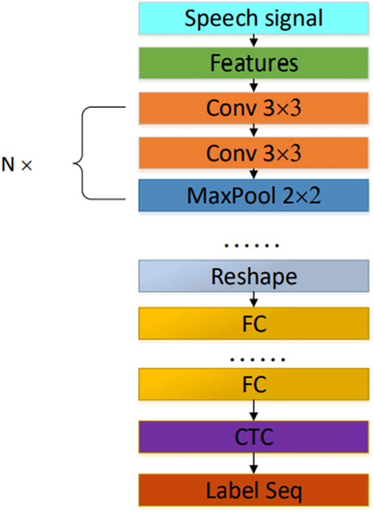
Figure 6: Configuration of CTC-CNN acoustic model

3  System Architecture

3.1 System Design

Fig. 7 portrays the architectural diagram of the hardware employed in this experiment. It comprises the ReSpeaker Mic Array v2.0.1 and display screen. The ReSpeaker Mic Array v2.0.1 is used to record voice data, and the recorded voice signals are compared with the voice database. The algorithm is processed, and calculated results are displayed on the display screen to display the words, sentences, or phrases after the speech is converted into text.

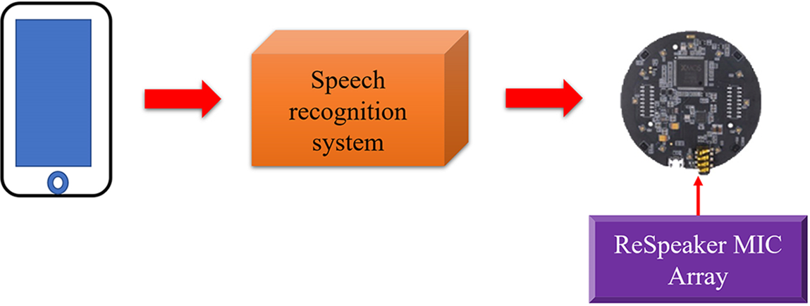
Figure 7: Hardware structure diagram

Fig. 8 shows the overall structure and flow chart of the speech recognition assistance system for language-impaired individuals. ReSpeaker Mic Array v2.0.1 records the speech signals of individuals with language impairments and extracts the recorded original voice recording files through a Python algorithm. Then, the algorithms extract voice features from the extracted raw data and yield the extracted features. The vectors are calculated algorithmically by the speech recognition system, which includes acoustic comparison and language decoding. The features are repeatedly compared and decoded in acoustic comparison and language decoding, until the calculated result is very similar or correct to the original intention of the speaker, i.e., it yields the intended output. The result is presented in the form of text to be displayed on the vehicle.

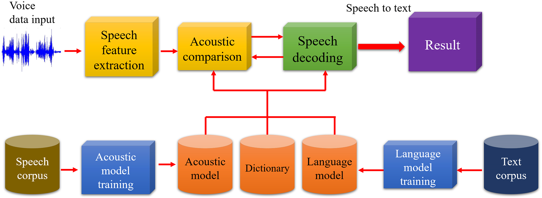
Figure 8: System structure diagram

The upper layer of acoustic comparison and language decoding is mainly divided into three parts, namely the acoustic model, pronunciation dictionary, and language model. Among them, the acoustic model uses the language corpus to train and adjust the acoustic model, enabling cross-comparison with the speaker’s pronunciation, words, and expressions to improve the accuracy of identification. The language model is generated in the same manner as the acoustic model. The language model is trained and adjusted through the text corpus, to establish common words or sentences, and even multi-languages.

3.2 ReSpeaker Mic Array v2.0.1

The radio hardware component used in this experiment is the ReSpeaker Mic Array v2.0.1 by SeeedStudio. This is an upgrade to the original ReSpeaker microphone array v1.0. The upgraded version is based on XMOS′ XVF-3000, which is a chip with significantly higher performance than the previously used XVSM-2000. The comparison of XVF-3000 and XVSM-2000 specifications is shown in Table 1.

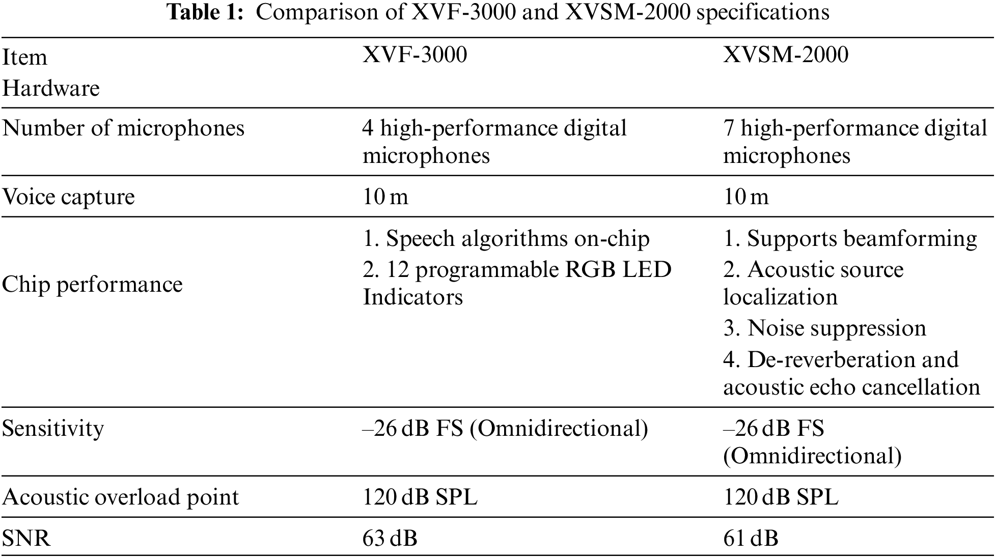
The microphones in this version have also been improved, with the number reduced to four compared to the seven in the first generation, and a significant performance increase. It can be used on many occasions, such as: smart speakers, smart voice assistant systems, voice conference systems, car voice assistants, etc. Compared with XVSM-2000, this new chipset adds a speech recognition algorithm to improve its performance. Added the following algorithms:

1.   Pick Up Voices From Far Away

     ●   Far-field voice capture enables you to capture and understand requests from up to 5 m away

2.   Focus On The Right Voice

     ●   DoA allows the device to know the direction of a source

     ●   BF allows the device to focus only on sounds that come from the target direction

     ●   Ignore background noise and chatter through NS

3.   Improved Voice Audio Quality

     ●   Reduces environmental voice echo with de-reverberation

     ●   Remove current audio output with AEC

The ReSpeaker Mic Array v2.0.1 module has numerous voice algorithms and features, and the maximum sampling rate is 16 kHz. This small chip has the benefits of numerous functions, as the module is equipped with XMOS’s XVF-3000 IC, which integrates advanced Digital signal processing (DSP) algorithms, including acoustic echo cancellation (AEC), beamforming, demixing, noise suppression, and gain control. It further supports USB Audio Class 1.0 (UAC 1.0) and has twelve programmable RGB color model (RGB) LED indicators for user freedom. The detailed specifications are shown in Table 1. Fig. 9 shows the ReSpeaker Mic Array v2.0.1 system diagram [19].

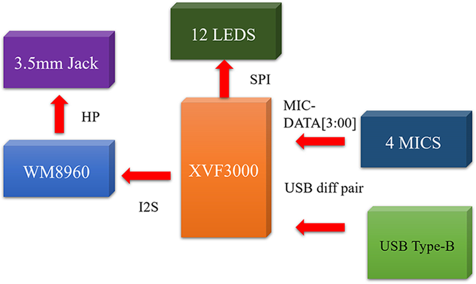
Figure 9: ReSpeaker Mic Array v2.0.1 system graph

3.3 System Technology Description

The study proposes an end-to-end speech enhancement architecture that (1) models the original speech waveform time domain signal, bypassing the phase processing operation in the traditional time-frequency conversion, and avoiding phase pollution, (2) transforms the one-dimensional time-domain speech signal, mapping it to a two-dimensional representation. More sufficient information is mined from the high-dimensional representation of the speech signal, and the codec network is subsequently used to learn the mapping from noisy to clean speech. This represents the dimensionality reduction and reconstruction into a time-domain waveform signal, (3) by combining the evaluation index with the loss function, the commonality and difference between different evaluation indexes are used to improve the perceptual ability of the model and obtain clearer speech.

The end-to-end model framework UNet [20] comprises the main structure of the framework, as shown in Fig. 10 [21]. The UNet neural network was initially applied for medical image processing and achieved good results. The main structure of UNet is composed of an encoding stage (left half of UNet) and a decoding stage (right half of UNet). Between each corresponding encoding stage and decoding stage, skip connections are used. The skip connections herein are not residual, as it is not the calculation method of the residual, but the method of splicing.

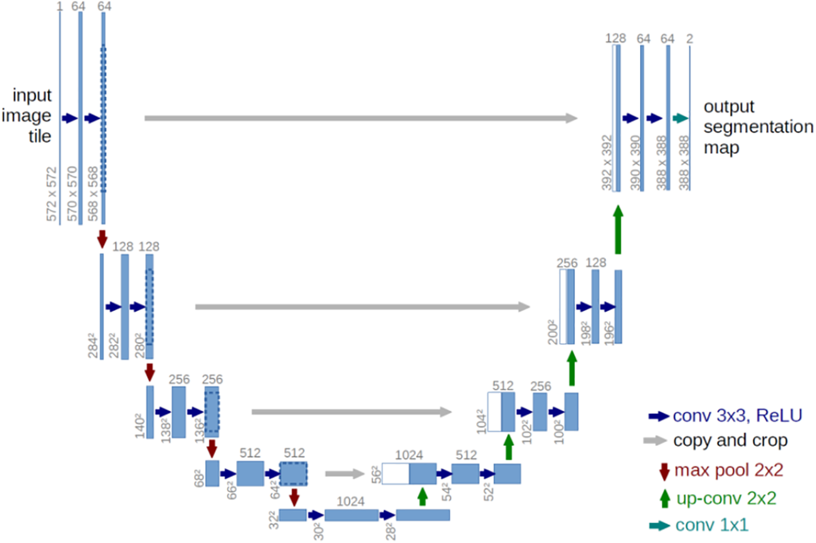
Figure 10: End-to-end model framework UNet

The structure of the model proposed in this study is shown in Fig. 11. The architecture consists of three parts, namely, preprocessing of the original audio signal, encoding and decoding module based on the UNet architecture, and post-processing of enhanced speech synthesis. By directly modeling the time domain speech signal, we avoid the defects and problems in the time-frequency transformation, and convert the one-dimensional signal into a two-dimensional signal through the convolution operation, such that the neural network can mine the speech signal in the high-dimensional space and deep representation. To reduce the number of parameters and the complexity of the model, the up-sampling operation in the decoding part of UNet here is not deconvolution, but bilinear interpolation [22].

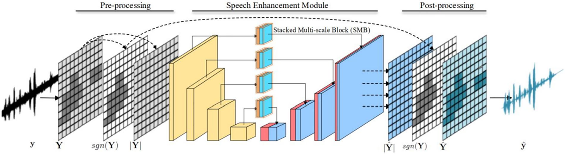
Figure 11: End-to-end speech enhancement framework

4  Analyses of Experimental Results

4.1 Basics Experimental Results

Experimental results are presented in Figs. 12a, 12b as screenshots of the web Graphical User Interface (GUI) interface. Fig. 12a shows the speaker saying “The weather is so nice today”, and the system successfully displays the speaker’s complete sentence. Fig. 12b shows the speaker saying “Good morning” twice in a row, but the recognition result is only successful one time; the result of the second time presents the situation of homophones. First, a voice recording is made on the ReSpeaker Mic Array v2.0.1. Subsequently, the algorithm rapidly performs voice recognition and displays the speaker’s incomplete or intermittent sentences on the vehicle, helping the language-impaired person to communicate smoothly and quickly with others [23].

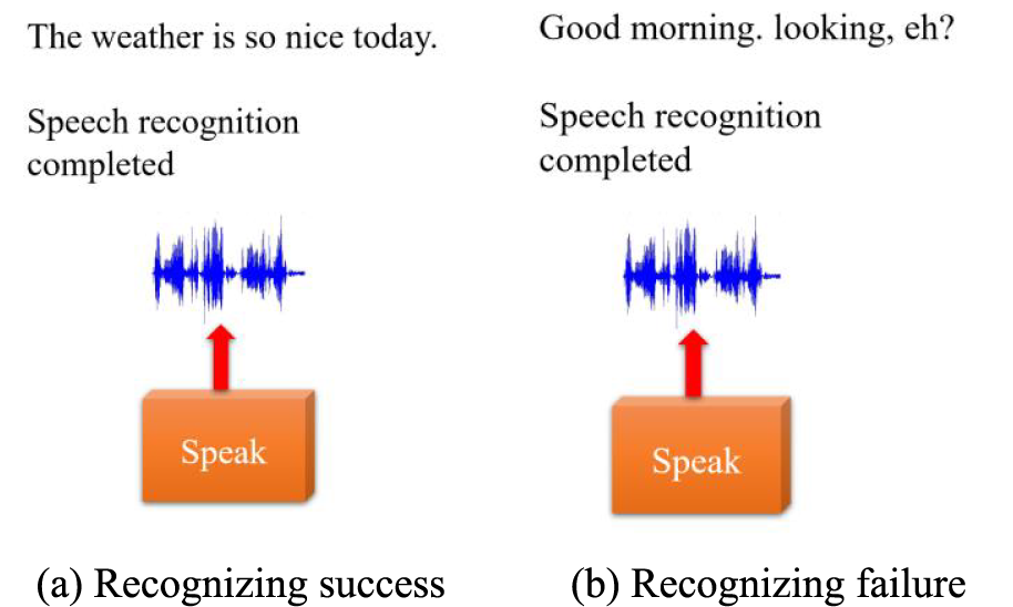
Figure 12: Recognizing experiment

4.2 Experimental Data Analysis

To train and verify the CTC-CNN baseline acoustic model, THCHS-30 and ST-CMDS speech datasets were used as training data sets, and the data sets are divided into training and test sets. The training results are shown in Figs. 13a and 13b, which show that after 54 epochs of training, the word error rate of the acoustic model training set is about 31%, and the word error rate of the test set is stable at about 43%. There is a certain overfitting phenomenon. Namely, the 43%-word error rate is difficult to put into practical application, such that it is necessary to optimize and adjust the network structure parameters to further improve the accuracy of the acoustic model.

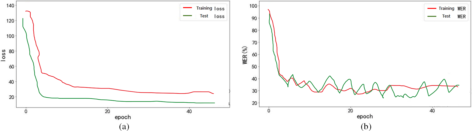
Figure 13: (a) Loss variation of baseline acoustic model (b) word error rate change of baseline acoustic model

Table 2 lists the recognition accuracies of several consecutive words. The results are obtained from 100 test datasets. When the speaker only speaks one word, the recognition accuracy is the highest, and the accuracy rate can reach 98.11%. In contrast, when the speaker utters sentences with more than five words, the recognition accuracy rate falls to only 93.77%. Sentences with more than five characters may cause the system to misdiagnose the words due to the speaker’s punctuation or if the pronunciation of the words is too similar, for example: “recognize speech” and “wreck a nice beach” have similar pronunciations in English, and “factors” with similar pronunciation in Chinese and “Sonic”, etc. In addition to the above-mentioned situations that affect the accuracy of identification, the environmental noise factor may also lead to a decrease in the accuracy of identification. Fig. 14 shows a prediction trend chart of various word count recognition accuracy rates.

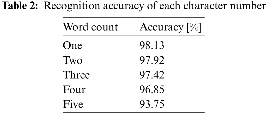
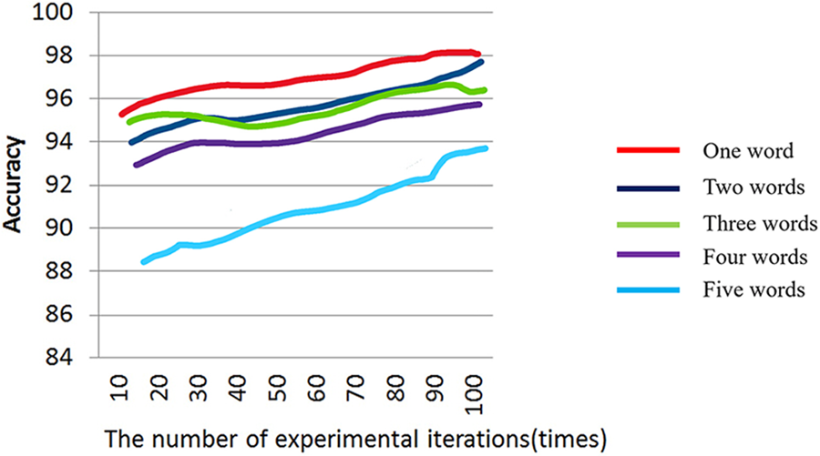
Figure 14: Prediction trend graph of various word count recognition accuracy rates

Therefore, this experiment also considers the surrounding ambient noise, and conducts 80 tests at each level of decibels, as shown in the following Table 3. Taking the noise of 80–90 dB as an example, at this level of noise, the accuracy rate is 88.18%, which represents the poorest performance among all levels. In contrast, at 40–60 dB, owing to less noise pollution, the accuracy rate is as high as 97.33%. Fig. 15 shows the prediction trend of environmental noise impact identification accuracy.

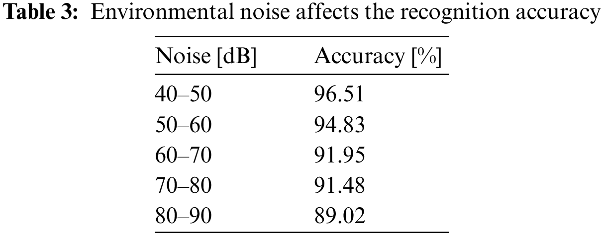
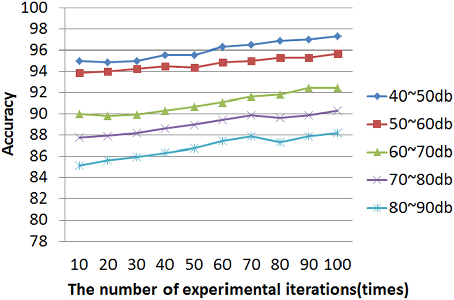
Figure 15: Prediction trend of environmental noise impact recognition accuracy

Because of the similarities in Chinese pronunciation, the recognition error rate of the system is expected to increase significantly. To this end, we designed this experiment based on the characteristics of Chinese consonants and vowels to verify their time-frequency map. There are 21 consonants and 16 vowels, respectively, in the Chinese phonetic alphabet. The forming of vowels mainly occurs by the change of mouth shape, while consonants are formed by controlling the flow of air through certain parts of the oral cavity or nasal cavity. Therefore, the energy of consonants is small, their frequency is high, and the time is short, and most of them appear before vowels. Conversely, vowels have higher energy, lower frequency, and longer duration, and usually appear after consonants or independently. The energy and frequency difference of vowels can be verified through time-frequency graph experiments, and this difference can be used to perform simple vowel identification [24].

4.3 Tuning and Optimization of Acoustic Models

The models are trained through continuous design and improvement of the relevant parameters of the acoustic model, and finally, the model with excellent performance is selected according to the evaluation index. The baseline acoustic model in this study faces challenges such as long training time, high error rate, and a certain degree of overfitting. Common optimization strategies for neural networks include dropout, normalization, and residual modules. Dropout was first proposed by Srivastava et al. in 2018, which can effectively solve the problem of overfitting. Normalization was first proposed by Segey Loffe and Christian Szegedy in 2020, which can speed up the model convergence and alleviate the overfitting problem to a certain extent. The residual module was proposed by Kaiming He et al. in 2022 [25], which solves the problem of gradient disappearance caused by the deepening of network layers.

The features of the neural network input generally follow the standard normal distribution, and generally perform well for shallow models. However, as the depth of the network increases, the nonlinear layer of the network will make the output results interdependent, and no longer meet a standard normal distribution. The problem of the output center offset will occur, which brings difficulties to the training of the network model. The training of deep models is particularly difficult. To solve the problem of model convergence, a normalization operation is added to the middle layer, i.e., a normalization process is performed on the output of each layer to make it conform to the standard normal distribution. Through this processing, the network input conforms to the standard normal distribution, which can be well-trained, thus speeding up the convergence speed. The data dimension processed by the convolutional neural network is a four-dimensional tensor, such that there are numerous normalization methods: layer normalization (LN), instance normalization (IN), group normalization (GN), batch normalization (BN), etc. [26].

Fig. 16 illustrates schematic diagrams of the normalizations for comparison. Taking a piece of voice data as an example, as the voice frequency range is roughly 250–3400 Hz, and the high frequency is 2500–3400 Hz, four intrinsic mode functions (IMF) component frequency diagrams are decomposed by the normalized comparison method, as shown in Figs. 17a–17d. From the density of the normalized amplitude value of each IMF component, the high-frequency region of speech is mainly concentrated in the first IMF component. Figs. 17a–17d indicate that the high-frequency region of the speech signal can be effectively extracted by empirical mode decomposition (EMD) decomposition. However, for the feature parameter extraction method of the high-frequency region, the traditional extraction algorithm is not suitable, and one must seek the high-frequency feature parameter extraction algorithm [27].

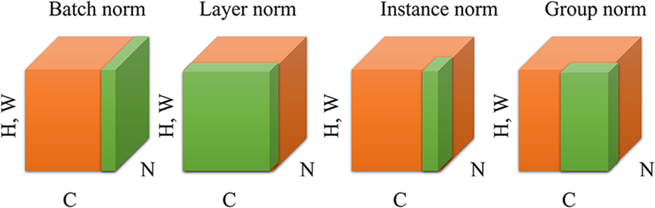
Figure 16: Contrast charts of applied normalization

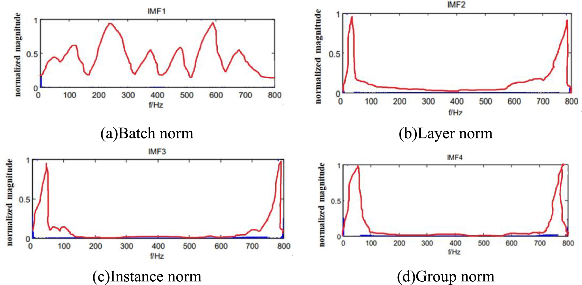
Figure 17: Contrast chart of normalizations based on IMF

Fig. 18 shows a schematic diagram of the Residual module, which transmits original input information to the output layer through a new channel opened on the network side. The Residual module directly transfers the input of the previous layer to a later layer by adding a congruent mapping layer. The principle of Dropout to suppress overfitting is to temporarily set some neurons to zero during network training, and ignore these neurons for parameter optimization, such that the network structure of each repeated operation training is different, to avoid network reliance on a single feature for classification and prediction. Dropout, a method of training multiple neural networks and then averaging the results of the entire set, instead of training a single neural network, increases the sparsity of the network model and improves its generalization.

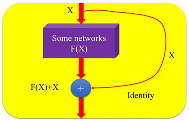
Figure 18: Schematic graph of residual module

Figs. 19a and 19b show the training comparison of the baseline acoustic model and improved acoustic model, respectively [28].

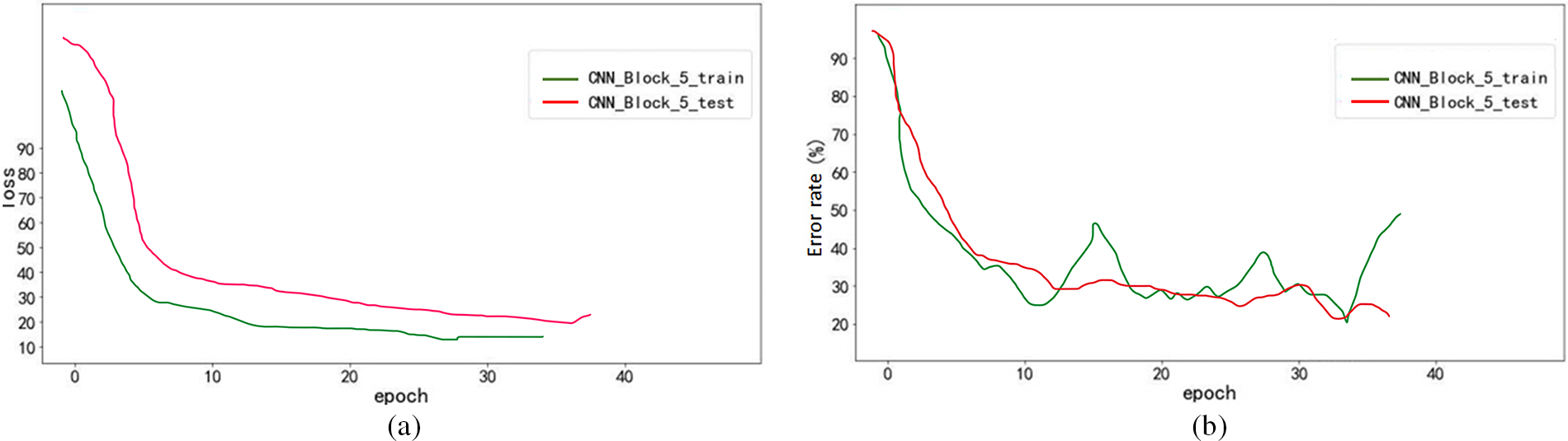
Figure 19: (a) Loss contrast of acoustic model; (b) contrast of WER of the acoustic model

Fig. 19b shows that by increasing the depth of the network model, the improved acoustic model reduces the WER by 3.5% on the test set compared to the baseline model. Although the error rate drops, the effect is still unsatisfactory. Fig. 19a shows that the improved acoustic model still faces the overfitting problem. Therefore, further optimization of this improved acoustic model is required. In the improved acoustic model, the number of network layers has reached 25. If the network layer continues to be deepened, the training time becomes too long, which likewise affects the decoding performance. To solve the overfitting problem, Dropout, and Batch Normalization (BN) layers are employed in the network model. The network model structure is shown in Fig. 20 [29].

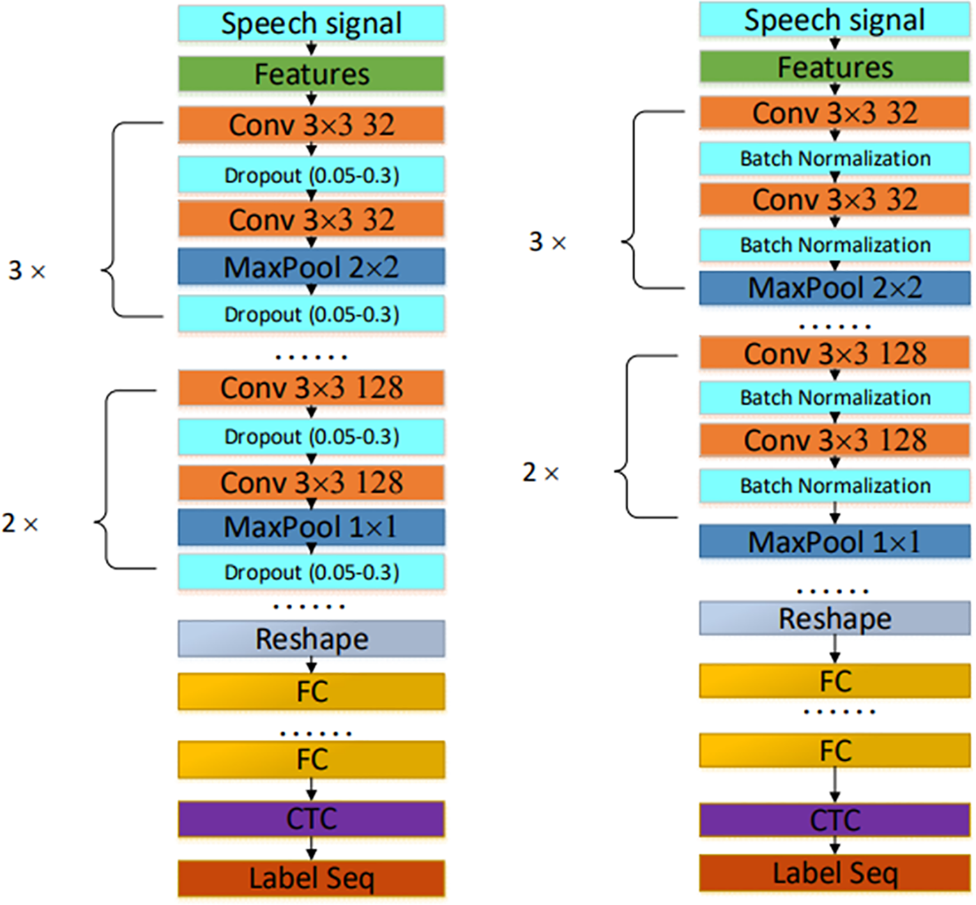
Figure 20: Contrast of structures between dropout and BN acoustic models

Figs. 21a and 21b show the training comparison diagrams of the Dropout and BN acoustic models.

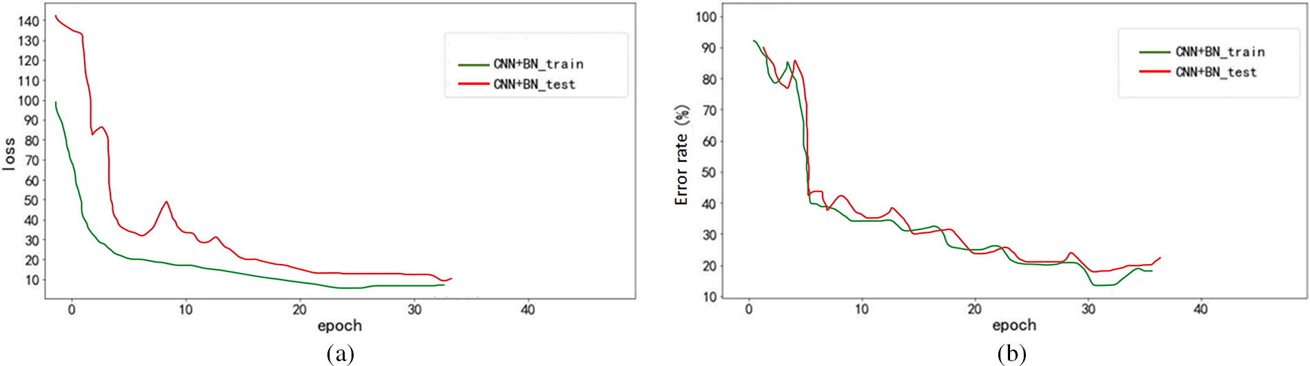
Figure 21: (a) Contrast of loss between dropout and BN acoustic models; (b) contrast of WER between dropout and BN acoustic models

Fig. 21a shows that both the Dropout and the BN acoustic models play a role in suppressing overfitting. However, as indicated in Fig. 21b, the error rate of the acoustic model using Dropout does not drop but rises instead, revealing the opposite effect. The acoustic model using BN effectively reduces the error rate, and at the same time accelerates the convergence, such that the training speed of the model is accelerated. The error rate of the BN acoustic model drops to 23.67%, indicating an 8% improvement over the baseline acoustic model. Considering the gradient vanishing problem that may be imposed by the deep convolutional neural network, the residual module is added based on the BN acoustic model, which is expected to further reduce the error rate. Fig. 22 shows the acoustic model with the added Residual module.

Figure 22: Acoustic model of residual plus BN

Fig. 23a shows that the Residual plus BN acoustic model has the fastest convergence speed among all models, i.e., the Residual module effectively alleviates the problem of gradient disappearance and speeds up the training speed of the model. As observed in Fig. 23b, the error rate of the model on the test set is reduced to 12.45%, which is 17% higher than the initial baseline acoustic model. An error rate of 13.52% is already an excellent result on the current scale of the dataset.

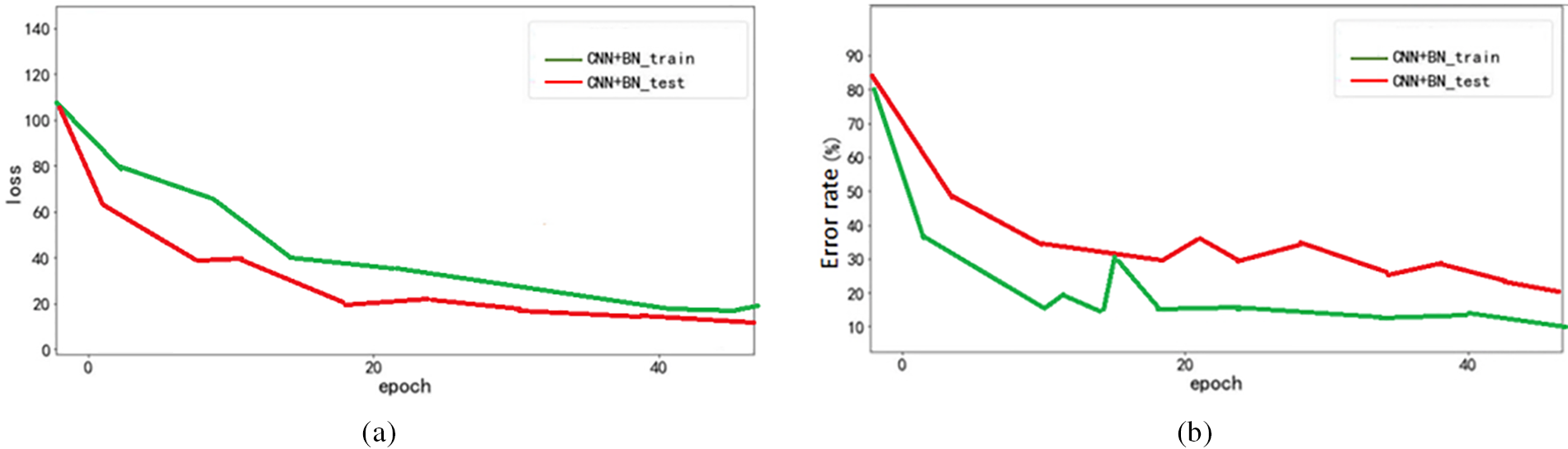
Figure 23: (a) Training loss graph of residual plus BN acoustic model; (b) WER change of residual plus BN acoustic model

According to all the above experiments, the experimental results show that each item of data in the experiment has a very good performance, and through the feedback of the experimental data, the experimental methods and procedures are continuously revised, and finally audio2text obtains very good performance.

5  Conclusions and Future Directions

In the speech recognition system, the acoustic model is an important underlying model, whose accuracy directly affects the performance of the entire system. This chapter introduces the construction and training process of the acoustic model in detail, and studies the CTC algorithm that plays an important role in the end-to-end framework. We constructed the CTC-CNN baseline acoustic model, and on this basis, carried out the optimization, reducing the error rate to about 18%, hence improving the accuracy. Finally, the selection of acoustic feature parameters as well as the selection of modeling units, the speaker’s speech speed, and other aspects was compared and verified, and the excellent performance of the CTCCNN_5 plus BN plus Residual model structure is further verified.

This study briefly introduces the historical development of deep learning and the most widely used deep learning models, and presents the development and current situation of these deep learning models in the field of speech recognition. Deep learning research is still in its developmental stage, and the main problems are: (1) training usually must solve a highly nonlinear optimization problem, which easily leads to many local minima in the process of training the network; (2) if the training takes too long, it will cause overfitting of the results. Thus, the use of deep neural networks to solve the robustness problem is currently the hottest topic in the field of speech recognition. In practical applications, the recognition rate of noisy speech is only about 85%, such that there is no stable, efficient, and universal system that can achieve a recognition rate of more than 95% for noisy speech. For future research on speech recognition, we believe that the best direction of development is brain-like computing. Only by continuously conforming to the characteristics of speech recognition of the human brain, can the recognition rate of speech be improved to a satisfactory level. However, the existing deep learning technology is far from sufficient to meet this requirement. How to better apply deep learning and meet the market demand for efficient speech recognition systems is a problem worthy of continued focus.

Acknowledgement: This research was supported by the Department of Electrical Engineering at National Chin-Yi University of Technology. The authors would like to thank the National Chin-Yi University of Technology, Takming University of Science and Technology, Taiwan, for supporting this research.

Funding Statement: The authors received no specific funding for this study.

Author Contributions: W. -T. S. is responsible for research planning and providing improvement methods. H. -W. K. and S. -J. H. is responsible for thesis writing and experimental verification.

Availability of Data and Materials: Data sharing not applicable to this article as no datasets were generated or analyzed during the current study.

Conflicts of Interest: The authors declare that they have no conflicts of interest to report regarding the present study.

References

1. K. Jambi, H. Al-Barhamtoshy, W. Al-Jedaibi, M. Rashwan and S. Abdou, “Speak-correct: A computerized interface for the analysis of mispronounced errors,” Computer Systems Science and Engineering, vol. 43, no. 3, pp. 1155–1173, 2022. [Google Scholar]

2. A. Das, J. Li, G. Ye, R. Zhao and Y. Gong, “Advancing acoustic-to-word CTC model with attention and mixed-units,” IEEE/ACM Transactions on Audio, Speech, and Language Processing, vol. 27, no. 12, pp. 1880–1892, 2019. [Google Scholar]

3. R. P. Bachate, A. Sharma, A. Singh, A. A. Aly, A. H. Alghtani et al., “Enhanced marathi speech recognition facilitated by grasshopper optimisation-based recurrent neural network,” Computer Systems Science and Engineering, vol. 43, no. 2, pp. 439–454, 2022. [Google Scholar]

4. S. Lu, J. Lu, J. Lin and Z. Wang, “A hardware-oriented and memory-efficient method for CTC decoding,” IEEE Access, vol. 7, pp. 120681–120694, 2019. [Google Scholar]

5. S. Darjaa, R. Sabo, M. Trnka, M. Rusko and G. Múcsková, “Automatic recognition of Slovak regional dialects,” in Proc. of 2018 World Symp. on Digital Intelligence for Systems and Machines (DISA), Kosice, Slovakia, pp. 305–308, 2018. [Google Scholar]

6. J. Tang, X. Chen and W. Liu, “Efficient language identification for all-language internet news,” in Proc. of 2021 Int. Conf. on Asian Language Processing (IALP), Singapore, pp. 165–169, 2021. [Google Scholar]

7. Z. Wang, Y. Zhao, L. Wu, X. Bi, Z. Dawa et al., “Cross-language transfer learning-based Lhasa-Tibetan speech recognition,” Computers, Materials & Continua, vol. 73, no. 1, pp. 629–639, 2022. [Google Scholar]

8. V. Bhardwaj, V. Kukreja, N. Kaur and N. Modi, “Building an ASR system for Indian (Punjabi) language and its evaluation for Malwa and Majha dialect: Preliminary results,” in Proc. of 2021 12th Int. Conf. on Computing Communication and Networking Technologies (ICCCNT), Kharagpur, India, pp. 1–5, 2021. [Google Scholar]

9. M. H. Changrampadi, A. Shahina, M. Badri Narayanan and A. N. Khan, “End-to-end speech recognition of Tamil language,” Intelligent Automation & Soft Computing, vol. 32, no. 2, pp. 1309–1323, 2022. [Google Scholar]

10. Z. Zhao and P. Bell, “Investigating sequence-level normalisation for CTC-like End-to-end ASR,” in Proc. of 2022 IEEE Int. Conf. on Acoustics, Speech and Signal Processing (ICASSP), Singapore, pp. 7792–7796, 2022. [Google Scholar]

11. A. Nakamura, K. Ohta, T. Saito, H. Mineno, D. Ikeda et al., “Automatic detection of chewing and swallowing using hybrid CTC/Attention,” in Proc. of 2020 IEEE 9th Global Conf. on Consumer Electronics (GCCE), Kobe, Japan, pp. 810–812, 2020. [Google Scholar]

12. H. Wu and A. K. Sangaiah, “Oral English speech recognition based on enhanced temporal convolutional network,” Intelligent Automation & Soft Computing, vol. 28, no. 1, pp. 121–132, 2021. [Google Scholar]

13. E. Yavuz and V. Topuz, “A phoneme-based approach for eliminating out-of-vocabulary problem Turkish speech recognition using hidden markov model,” Computer Systems Science and Engineering, vol. 33, no. 6, pp. 429–445, 2018. [Google Scholar]

14. T. Moriya, H. Sato, T. Tanaka, T. Ashihara, R. Masumura et al., “Distilling attention weights for CTC-based ASR systems,” in Proc. of 2020 IEEE Int. Conf. on Acoustics, Speech and Signal Processing (ICASSP), Barcelona, Spain, pp. 6894–6898, 2020. [Google Scholar]

15. H. Zhou, J. Du, Y. Zhang, Q. Wang, Q. F. Liu et al., “Information fusion in attention networks using adaptive and multi-level factorized bilinear pooling for audio-visual emotion recognition,” IEEE/ACM Transactions on Audio, Speech, and Language Processing, vol. 29, pp. 2617–2629, 2021. [Google Scholar]

16. Y. Cai, L. Li, A. Abel, X. Zhu, D. Wang et al., “Deep normalization for speaker vectors,” IEEE/ACM Transactions on Audio, Speech, and Language Processing, vol. 29, pp. 733–744, 2020. [Google Scholar]

17. G. Kim, H. Lee, B. K. Kim, S. H. Oh and S. Y. Lee, “Unpaired speech enhancement by acoustic and adversarial supervision for speech recognition,” IEEE Signal Processing Letters, vol. 26, no. 1, pp. 159–163, 2019. [Google Scholar]

18. Y. Lin, D. Guo, J. Zhang, Z. Chen and B. Yang, “A unified framework for multilingual speech recognition in air traffic control systems,” IEEE Transactions on Neural Networks and Learning Systems, vol. 32, no. 8, pp. 3608–3620, 2021. [Google Scholar] [PubMed]

19. T. Kawase, M. Okamoto, T. Fukutomi and Y. Takahashi, “Speech enhancement parameter adjustment to maximize accuracy of automatic speech recognition,” IEEE Transactions on Consumer Electronics, vol. 66, no. 2, pp. 125–133, 2020. [Google Scholar]

20. L. Ren, J. Fei, W. K. Zhang, Z. G. Fang, Z. Y. Hu et al., “A microfluidic chip for CTC whole genome sequencing,” in Proc. of 2019 IEEE 32nd Int. Conf. on Micro Electro Mechanical Systems (MEMS), Seoul, Korea (Southpp. 412–415, 2019. [Google Scholar]

21. C. Yao, M. Hu, Q. Li, G. Zhai and X. P. Zhang, “Transclaw U-Net: Claw U-Net with transformers for medical image segmentation,” in Proc. of 2022 5th Int. Conf. on Information Communication and Signal Processing (ICICSP), Shenzhen, China, pp. 280–284, 2022. [Google Scholar]

22. L. H. Juang and Y. H. Zhao, “Intelligent speech communication using double humanoid robots,” Intelligent Automation & Soft Computing, vol. 26, no. 2, pp. 291–301, 2020. [Google Scholar]

23. T. A. M. Celin, G. A. Rachel, T. Nagarajan and P. Vijayalakshmi, “A weighted speaker-specific confusion transducer-based augmentative and alternative speech communication aid for Dysarthric speakers,” IEEE Transactions on Neural Systems and Rehabilitation Engineering, vol. 27, no. 2, pp. 187–197, 2019. [Google Scholar]

24. Y. Takashima, R. Takashima, T. Takiguchi and Y. Ariki, “Knowledge transferability between the speech data of persons with dysarthria speaking different languages for Dysarthric speech recognition,” IEEE Access, vol. 7, pp. 164320–164326, 2019. [Google Scholar]

25. Y. Yang, Y. Wang, C. Zhu, M. Zhu, H. Sun et al., “Mixed-scale UNet based on dense atrous pyramid for monocular depth estimation,” IEEE Access, vol. 9, pp. 114070–114084, 2021. [Google Scholar]

26. N. Y. H. Wang, H. L. S. Wang, T. W. Wang, S. W. Fu, X. Lu et al., “Improving the intelligibility of speech for simulated electric and acoustic stimulation using fully convolutional neural networks,” IEEE Transactions on Neural Systems and Rehabilitation Engineering, vol. 29, pp. 184–195, 2021. [Google Scholar] [PubMed]

27. R. E. Jurdi, C. Petitjean, P. Honeine and F. Abdallah, “BB-UNet: U-Net with bounding box prior,” IEEE Journal of Selected Topics in Signal Processing, vol. 14, no. 6, pp. 1189–1198, 2020. [Google Scholar]

28. R. Haeb-Umbach, J. Heymann, L. Drude, S. Watanabe, M. Delcroix et al., “Far-field automatic speech recognition,” Proceedings of the IEEE, vol. 109, no. 2, pp. 124–148, 2021. [Google Scholar]

29. S. Latif, J. Qadir, A. Qayyum, M. Usama and S. Younis, “Speech technology for healthcare: Opportunities, challenges, and state of the art,” IEEE Reviews in Biomedical Engineering, vol. 14, pp. 342–356, 2021. [Google Scholar] [PubMed]