Adaptive Momentum-Backpropagation Algorithm for Flood Prediction and Management in the Internet of Things

1  Introduction

Flooding has been a devastating aspect of human civilization for many centuries, as it affects the lives and livelihoods of millions [1,2]. Therefore, effective flood early warning systems are essential to reduce the losses from floods [3,4]. Monitoring floods enable authorities to make better decisions to reduce the impact of floods. Due to climate change, traditional disaster management systems are unable to effectively predict the initial occurrence of floods [5]. As climate change continues to worsen, the frequency and intensity of flooding events are projected to rise, posing challenges to traditional disaster management systems [6]. Forecasting the onset of heavy rains early is crucial in limiting the damage caused by flooding [7,8]. Although several existing systems can predict rainfall in advance, they often fall short due to the constantly changing climate [9]. In such a scenario, developing more accurate, timely, and reliable flood prediction systems is of paramount importance to save lives, minimize property damage and enhance the resilience of communities to flooding events.

The power of IoT in enhancing flood management is derived from its ability to provide a seamless data collection, communication, and analysis platform. The integration of machine learning algorithms and big data applications with IoT devices holds the potential to enhance flood forecasting, early warning systems, monitoring, and management [10–12]. In the past few decades, researchers have proposed different flood prediction models that utilize IoT and Artificial Intelligence (AI) technologies. These models encompass a range of approaches, including simple correlations based on stage-discharge data, deterministic models, Artificial Neural Networks (ANN), and fuzzy logic techniques [13–21].

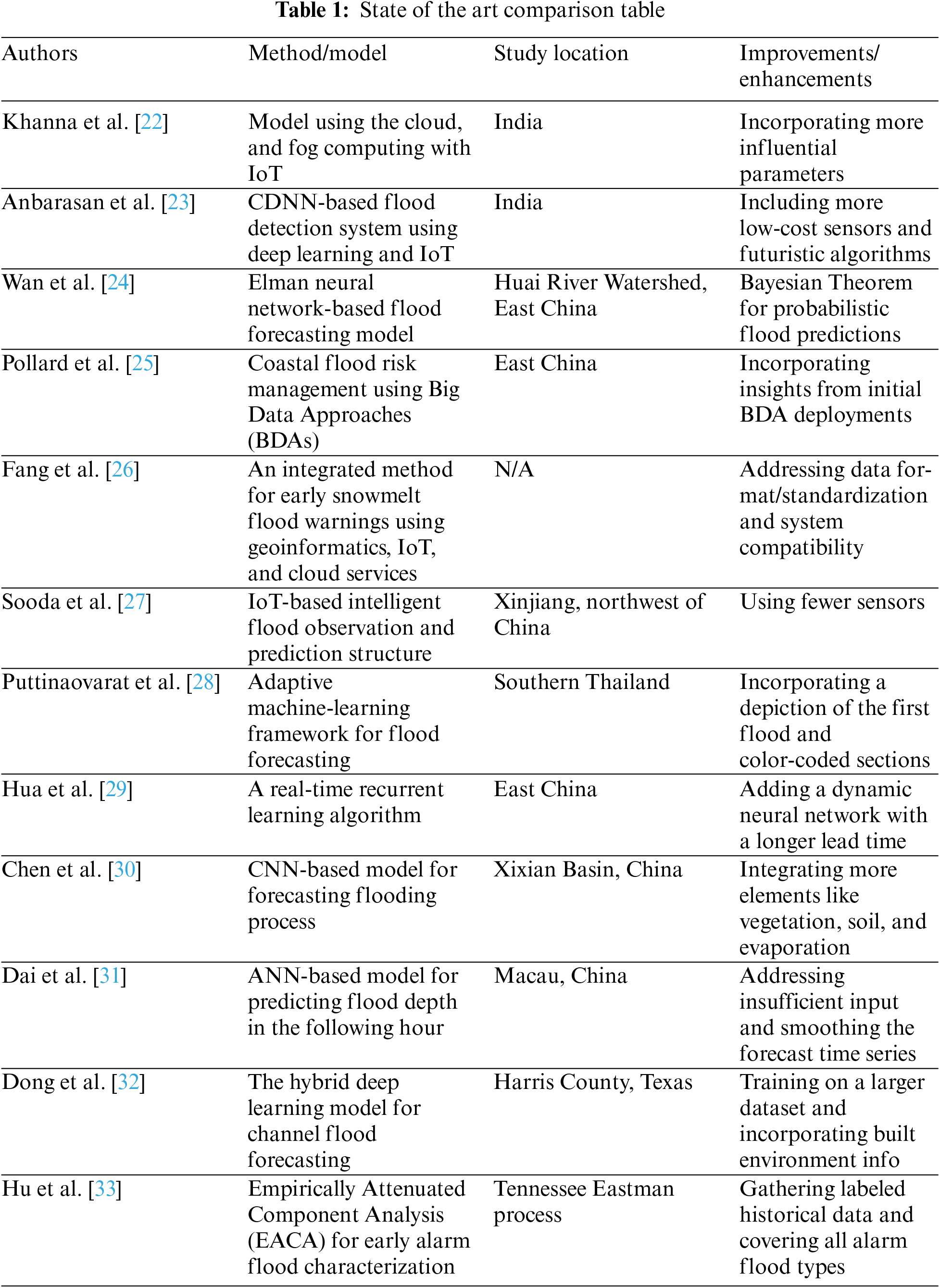
Khanna et al. [22] developed a flood prediction system using cloud computing, mobile edge computing, fog computing, and the IoT. They used sensory data to create the multi-model computing architecture. Anbarasan et al. [23] proposed a flood detection system based on Convolutional Deep Neural Networks (CDNN), deep learning, and the IoT. They pre-processed the data and developed rules for flood risk categories. Wan et al. [24] created a flood forecasting model using Elman neural networks. They trained the models with a real-time recurrent learning algorithm and used the Bayesian Theorem for probabilistic flood predictions. Pollard et al. [25] focused on coastal flood risk management and explored the use of Big Data Approaches in flood risk assessment and emergency response protocols.

Fang et al. [26] developed an integrated method for early snowmelt flood warnings using geoinformatics, IoT, and cloud services. They established an Integrated Information System for improved early-warning and snow-melt flood simulation processes. Sooda et al. [27] suggested an IoT-based flood observation and prediction structure using Big Data and High-Performance Computing. They optimized sensor placement and energy conservation using social network analysis and dimensionality reduction techniques. Puttinaovarat et al. [28] described a flood forecasting system that utilizes hydrological, crowd-sourced, meteorological, and geographic big data. They proposed incorporating the depiction of the first flood and extending it to the user’s current position. Hue et al. [29] developed a flood forecasting model using elman neural networks for the Xianghongdian reservoir in East China. The model is trained with a real-time recurrent learning algorithm and meets the required precision.

Chen et al. [30] developed a flooding process forecasting model using Convolution Neural Networks and two-dimensional convolutional operations. They focused on the rainfall characteristics in the Xixian basin. Dai et al. [31] proposed an artificial neural network-based model for predicting flood depth in Macau, China. They acknowledged the need for improvements in input, model structure, forecasted values, and the smoothness of the forecast time series. Dong et al. [32] proposed a hybrid deep learning model, a fast, accurate, stable, and tiny gated recurrent neural network-fully convolutional network for forecasting channel flood changes using historical spatial-temporal data. They suggested improvements such as training on larger datasets and incorporating built environment information. Hu et al. [33] proposed an empirically attenuated component analysis method for the early characterization of alarm floods. Their work highlighted the importance of incorporating labeled historical data and including all possible types of alarm floods in the training dataset.

Table 1 presents a comparison of state-of-the-art flood prediction models. Despite the advancement in flood prediction models, certain research gaps persist. Existing models often suffer from inefficient parameter tuning, limiting their accuracy. They also struggle with scalability issues, hindering their ability to process large volumes of weather data. High latency and reduced responsiveness due to inefficient data management pose another challenge. Moreover, many models grapple with the complexity of analyzing large-scale data and exhibit limited adaptability, being designed for specific scenarios or locations, which restricts their broad applicability.

Traditional approaches to data management often face difficulties in handling the real-time nature of meteorological data and the intricate relationships between various environmental factors [34–37]. Meteorological data is characterized by its dynamic and time-sensitive nature. It is collected from numerous sensors and stations across different geographical locations, providing updates at frequent intervals [38,39]. Managing such real-time data requires efficient data ingestion, storage, and processing mechanisms that can handle the high data velocity and volume associated with meteorological observations. Furthermore, meteorological data is multidimensional and interconnected with complex relationships between different environmental factors. Variables such as temperature, humidity, wind speed, atmospheric pressure, and precipitation are interconnected and influence each other. Capturing and understanding these complex relationships is crucial for accurate flood prediction and management [40]. To address these challenges, this research proposes a Multilayer High-End Computing Architecture (MLCA) that incorporates fog and cloud computing technologies. This advanced architecture aims to enhance the efficiency of handling large datasets, leading to more accurate flood prediction models.

ANN models are effective in analyzing time-series data and capturing complex relationships between environmental factors, which are crucial in flood prediction. However, large datasets can pose challenges for machine learning models, such as the need for more computational resources and the risk of overfitting [41,42]. To overcome these challenges, the proposed approach combines two learning algorithms: The adaptive momentum (AM) algorithm and the backpropagation (BP) algorithm. The AM algorithm dynamically adjusts the learning rate during the training process based on the gradient information. This adjustment allows for faster convergence and better optimization of the ANN model. On the other hand, the BP algorithm updates the weights and biases of the ANN based on the error between the predicted and actual outputs. By incorporating the AM and BP algorithms, the procedure aims to enhance the efficiency and effectiveness of the ANN model in flood prediction. It helps the model process large datasets more efficiently and improve the accuracy of the predictions by adjusting the learning rate and updating the model’s parameters based on the prediction errors. The important research contributions of this paper are summarized as follows:

Proposed Multilayer High-End Computing Architecture (MLCA) for efficient handling of large datasets in flood prediction models.

Combination of adaptive momentum (AM) and backpropagation (BP) algorithms to improve efficiency and accuracy of Artificial Neural Network (ANN) models in flood prediction.

Addressing challenges of processing large datasets in flood prediction by dynamically adjusting learning rate and updating model parameters.

The layout of this article is delivered as follows: Section 2 describes the proposed methodology along with a layered architecture description, deep analysis of existing flood prediction models, detailed High-End Computing Architecture (MLCA), and hybridized BP model. Section 3 provides the experimental results of the proposed system. Section 4 concludes the paper.

2  Proposed Methodologies

A reliable flood forecasting and monitoring system are dependent on several elements including reliable meteorological data collecting, effective data analysis, timely result alerts, and an intuitive user interface. The four-layered design proposed for an efficient flood forecasting system is illustrated in Fig. 1. The proposed architecture is composed of four layers: the lowest layer is referred to as the sensing layer or Internet of Things layer, the second layer is referred to as the Fog Computing Layer, the layer above the Fog Computing Layer is referred to as the Data Analysis Layer and the topmost layer is referred to as the Presentation Layer or user interface.

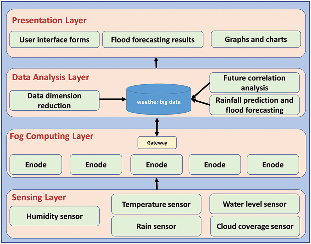
Figure 1: Four-layered architecture for weather big data analysis and flood management

2.1 Sensing Layer

The sensing layer consists of a broad IoT network architecture that is connected to a variety of IoT weather smart sensors, such as cameras, sensors, and other monitoring devices. This layer generates massive amounts of large heterogeneous data.

Temperature sensing and humidity: To facilitate modeling, the sensor node monitors the temperature in degrees Celsius in the region in which it is monitored using a DHT11 sensor. This sensor is a capacitive-type humidity and temperature sensor that measures the surrounding air and provides temperature in degrees Celsius and relative humidity in percentage terms. The temperature has a small impact on rainfall in general. A high temperature implies the possibility of torrential rains, while a moderate temperature indicates a decent chance of precipitation. Low temperatures imply a minimal probability of rain. Static humidity sensing nodes quantify the atmosphere’s relative humidity in percentage terms. The general trend indicates that when the amount of humidity increases, the likelihood of rain increases as well. In this research, the DHT11 sensor was employed for both temperature and humidity sensing, providing an efficient and accurate method for monitoring these weather parameters.

Sensing of air pressure: The sensor nodes deployed to measure air pressure in millibars. The following points demonstrate how pressure affects weather conditions. If the air pressure suddenly increases, it suggests that the weather is clear and the temperature is about to fall. A rise in air pressure indicates that the weather is improving or that the conditions will remain stable. If atmospheric pressure remains constant, meteorological conditions remain constant as well. When atmospheric pressure gradually decreases, it suggests that the weather will be moist and there is a chance of rain. If the air pressure rapidly lowers, thunderstorms or heavy rains are likely.

Sensing of humidity: Static humidity sensing nodes quantify the atmosphere’s relative humidity in percentage terms using a DHT11 sensor. This sensor is a capacitive-type humidity and temperature sensor that measures the surrounding air and provides relative humidity in percentage terms. The general trend indicates that when the amount of humidity increases, the likelihood of rain increases as well.

Sensing of the water level: The water level, indicated in feet or cubic centimeters, shows the maximum amount of water that can be incorporated into a reservoir without overflowing or causing a hazard. A low value implies that the reservoir is still capable of handling additional flowing or rainwater. In this research, ultrasonic sensors were employed to measure the water level. Ultrasonic sensors emit high-frequency sound waves and measure the time it takes for the sound waves to bounce back from the water surface, calculating the distance to the water surface accordingly.

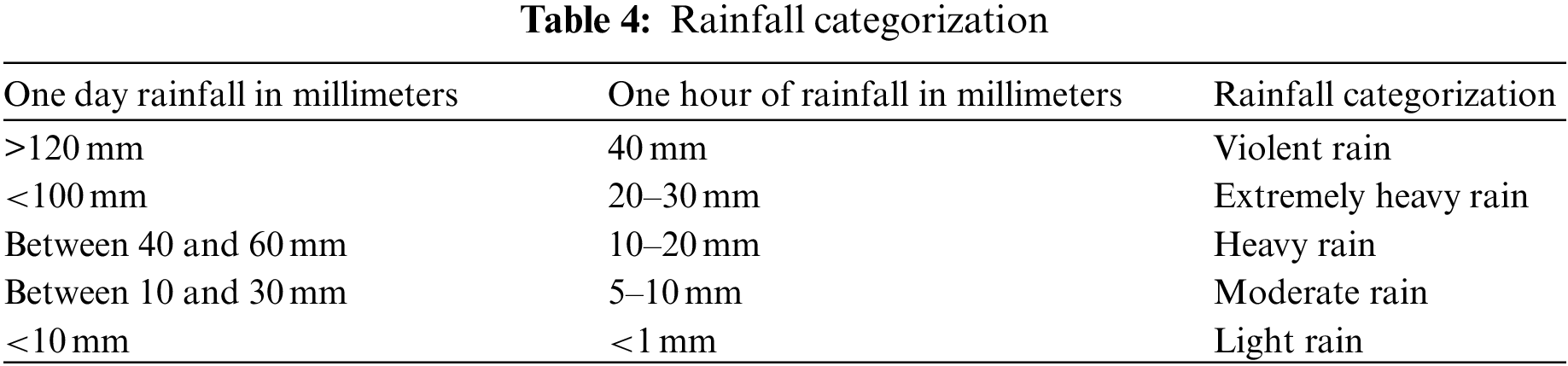
Sensing of rainfall: The rainfall attribute is indicated in millimeters (mm) of rain and is determined by the use of a network of fixed rainfall measurement sensors, specifically optical rain gauges, located at strategic locations around the area. Optical rain gauges use infrared or laser beams to detect raindrops falling through a sensing area, estimating the rainfall rate based on the number and size of the raindrops. Depending on the amount of rainfall, it is described as severe rainfall, very heavy rainfall, heavy rainfall, moderate rainfall, or light rainfall. The categorizing of rainfalls is done on a day-by-day and hour-by-hour basis.

2.2 Fog Computing Layer

To increase the processing capability of the proposed approach’s data analysis module, a fog layer is inserted between the edge and cloud layers. These fog nodes are found in a variety of geographic regions. It offers the memory, computing capability, storage, and resources required to handle the sensing layer’s data [43]. The data analysis layer will utilize the cloud to store and process data supplied by IoT devices. As seen in Fig. 1, data will be transported from IoT devices to cloud computing via a network of multiple network devices, which may include encodes and gateways. When real-time flood levels are forecast using a data analysis layer on a cloud computing infrastructure, the system will incur latency due to the number of steps required for data to transit. This configuration has the potential to drastically reduce the system’s latency.

2.3 Data Analysis Layer (Cloud Computing Layer)

The third layer is responsible for further processing and analyzing the aggregated data from the fog computing layer. It employs advanced algorithms, machine learning techniques, and big data analytics to predict and assess flood risks, identify potential threats, and generate actionable insights. Cloud computing provides scalability and the resources needed to handle large volumes of data and complex computations effectively.

2.3.1 Data Pre-Processing

In artificial intelligence, data pre-processing involves removing unnecessary data before feature extraction that has no impact on prediction results. Data pre-processing can significantly increase the training efficiency and precision of all AI algorithms. Weather data values are normally obtained through weather sensors, and the data collecting procedure is semi-automated. As a result of sensor failure and human mistakes, there is a possibility of having irrelevant and redundant data in weather data. Therefore, in this study, weather data are pre-processed to enhance the efficacy of flood prediction. First, in pre-processing, the dimension of the input is lowered by removing redundant data, allowing the ANN model to learn more intelligence from the least amount of data. Second, correlation analysis is performed to identify the data that influence the prediction.

2.3.2 Data Dimension Reduction

Due to the advancement of technology, weather monitoring has been computerized. As a result, multidimensional weather data is generated daily. In this multi-dimensional meteorological data, many hidden details forecast the upcoming weather patterns. However, AI algorithms struggle to learn from multidimensional weather data due to data dimensions. Therefore, in this study, principal component analysis was employed to reduce the obstacles caused by data dimension. The primary purpose of Principal Component Analysis (PCA) is to extract more information from fewer variables. It also reduces the dimension of the data and the problem’s complexity. In this study, the following formula is used to reduce the data dimension:

Y¯=∑i=1nD, 1≤i≤n(1)

The data dimension is denoted by D=(D1, D2,…,Dn). The actual number of data variables in the data collection is denoted by X=(X1,X2,…,Xn) and (Y¯=Y¯1,Y¯2,…,Y¯n) is the new data variables produced by the PCA.

In general, redundant features not only decline the prediction accuracy but also increase the training complexity. Obviously, due to geographical location and climatic change, there will be variations in the weather data’s features. Therefore, the correlation between inputs and predicted results (class) must be analyzed. The correlation analysis between the major meteorological parameters of this study is calculated using formula (2). The results of the correlation analysis are presented in Table 2.

Cxy=cov(x,y)σxσy(2)

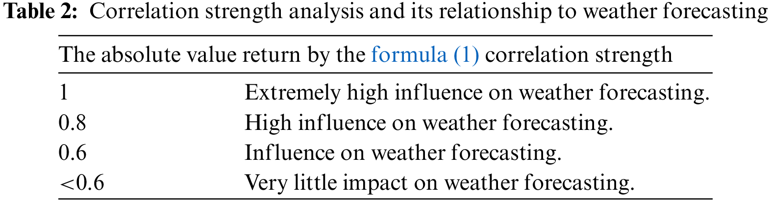
Formula (2) represents the correlation coefficient (Cxy), which is determined by dividing the covariance (cov(x,y)) between the variables by the product of their standard deviations (σx and σy).

cov(x,y)=E(xy)−E(x)E(y)(3)

The covariance between the features and the class, cov(x, y), is computed using formula (3), where E(xy) represents the expected value of the product of x and y, and E(x) and E(y) denote the expected values of x and y, respectively.

σx=E(x2)−E2(x)(4)

σy=E(y2)−E2(y)(5)

Formulas (4) and (5) calculate the standard deviations (σx and σy) of the features and the class, respectively. These values represent the square root of the differences between the expected values of the squares E(x2) and E(y2) and the squares of the expected values E2(x) and E2(y).

2.4 Data Set

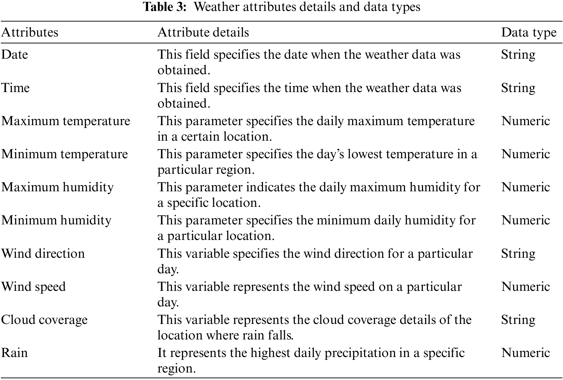
In order to train the forecast model, data were collected from the Regional Meteorological Centre in Chennai. This dataset consists of weather data (maximum temperature, minimum temperature, maximum humidity, minimum humidity, rain, wind direction, wind speed, and cloud coverage) recorded from 2014 to 2019 in various places in Chennai. The dataset’s detailed information is summarized in the table below. The class label for this data set is the rain attribute. This study divides the meteorological data set into four categories based on the amount of precipitation. When trained in this approach, errors and complexities during training can be reduced to a certain level. Accordingly, rainfall intensity below 2.5 millimeters per hour is classified as the first category, rainfall intensity between 2.5 millimeters and 8 millimeters per hour as the second category, rainfall intensity above 8 millimeters per hour as the third category, and rainfall intensity above 40 millimeters per hour as the fourth category. These data categories are labeled as light rain, moderate rain, heavy rain, and severe rain. The weather data set is detailed in Table 3.

2.5 Study Area

Chennai is located between approximately 12°50′4′′N and 13°17′24′′N in latitude, and between approximately 79°58′53′′E and 80°20′12′′E in longitude. It is approximately 6.7 m above sea level. The majority of Chennai is below sea level. Chennai, the fourth largest city in India approximately seven and a half million people living in the city continued to battle with the periodic floods and droughts. Chennai Corporation is organized into fifteen zones, each of which has 200 wards. Certain areas in Chennai suffer from poor drainage facilities during the monsoon season due to their huge topography. Climate change and global warming have considerably increased the amount of precipitation in Chennai over the past two decades, therefore Chennai has been chosen as the study area of this research. Every year, the northeast monsoon contributes up to 60% of the yearly rainfall to Chennai and its neighboring areas. During the northeast monsoon, Chennai’s coastline districts are frequently flooded. Between 1943 and 2015, six catastrophic floods completely wrecked the city of Chennai. Especially, floods in 1943, 1978, 2005, and 2015 wreaked havoc on Chennai and its surrounding areas. Two major rivers, Koovam and Adyar split Chennai into many regions. Due to recent urban expansion and development, the major industries of Chennai, particularly the Information Technology (IT) sector, have established themselves on the banks of these rivers. These rivers are prone to flooding as a result of sudden high rainfall, which can cause significant harm to employees and businesses. Figs. 2a–2c show Chennai’s flood-prone zones before and after industrial revaluation and urbanization. Figs. 2b and 2c compare the flood-prone areas in Chennai before and after industrialization. It clearly shows that the flood-prone areas increased significantly after industrialization, indicating the considerable impact of human actions on the city’s vulnerability to floods.

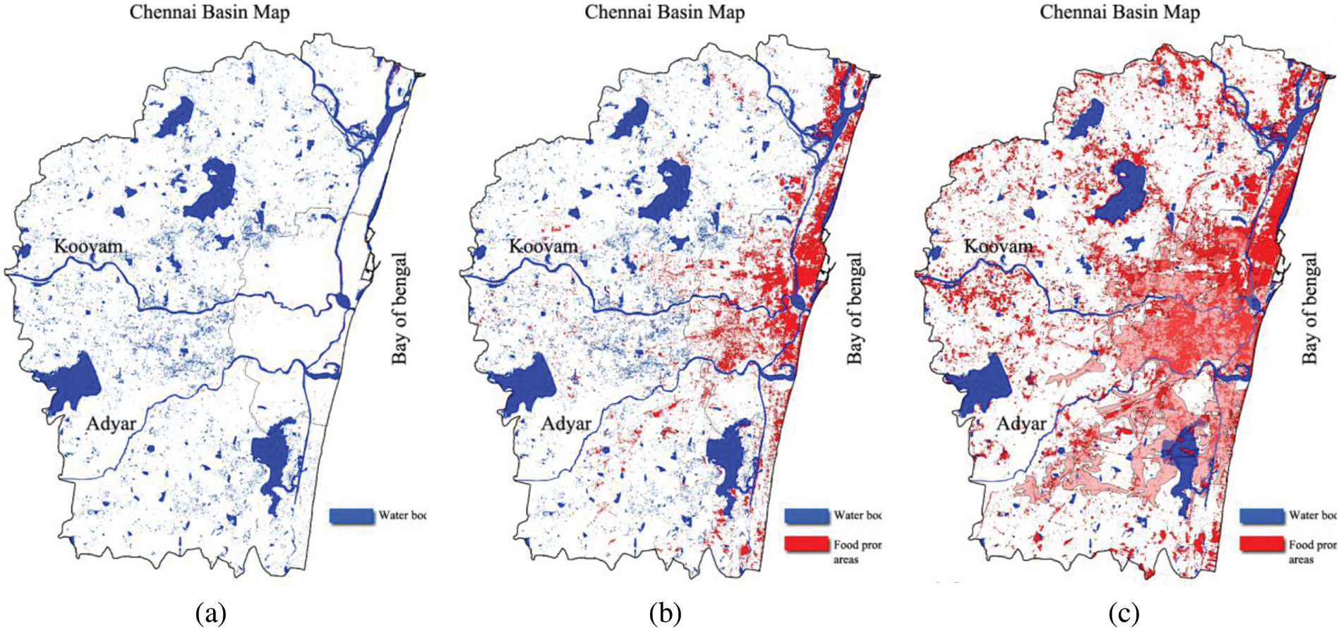
Figure 2: (a) Chennai basin map. (b) Chennai basin map before the industrial revolution. (c) Chennai basin map after the industrial revolution

2.6 Data Analysis Layer

Artificial Neural Networks (ANNs) are machine learning models inspired by the structure and function of biological nervous systems, including neurons and synapses [44,45]. ANNs are widely used for predicting future values based on historical time series data. They offer numerous advantages, such as robustness and simplicity, making them popular for time series prediction compared to other machine learning models.

Fig. 3 illustrates the general architecture of an ANN. ANNs can be trained for regression or classification tasks due to their flexible architecture. In this study, a system using ANN is developed to forecast flash floods based on historical daily rainfall time series data. The ANN aims to model a set of N input variables and M output variables (Y) using various activation functions. The input layer of the feed-forward network takes the time series data and maps it to artificial neurons, which are determined through backpropagation. The architecture of feed-forward networks comprises three layers: the input layer, the hidden layer, and the output layer. The number of hidden neurons can vary depending on the complexity of the task.

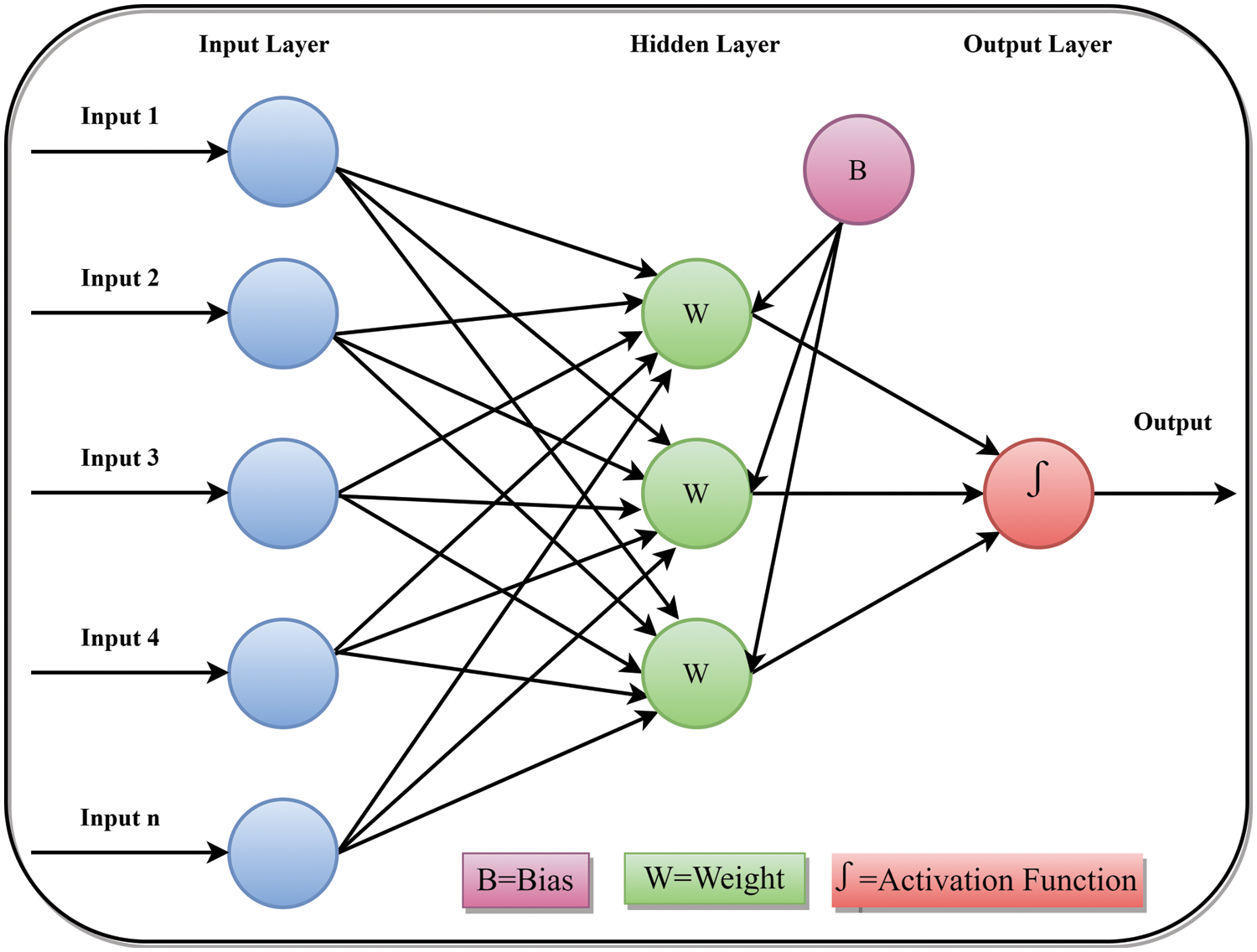
Figure 3: Graphical representation of the ANN architecture

In this study, ten meteorological variables contributed as inputs for the ANN model. These factors include the date, the time, the maximum temperature, the minimum temperature, the maximum humidity, the minimum humidity, the wind direction, the wind speed, the cloud cover, and the likelihood of rain (all these are explained in Table 3). The selected factors play a significant role in influencing flood conditions and improving the accuracy of the ANN model, as explained below:

1.    Date and time: Seasonal variations and daily fluctuations in meteorological conditions can affect flood risk. Including date and time as input variables help the model capture these variations and their impact on flood events.

2.    Maximum and minimum temperature: Temperature affects the rate of evaporation and precipitation, which in turn, influences the water cycle and flood risk. Using temperature data allows the model to learn the relationship between temperature and flood events.

3.    Maximum and minimum humidity: Humidity is a measure of the amount of water vapor in the atmosphere. High humidity levels can lead to increased precipitation, potentially increasing the risk of floods. Incorporating humidity data enables the model to understand the link between humidity and flood events.

4.    Wind direction and speed: Wind can affect the distribution of rainfall and the movement of floodwater. Including wind data in the model helps capture the influence of wind on flood risk.

5.    Cloud cover: Cloud cover can impact the amount of precipitation, with increased cloud cover potentially leading to higher rainfall and flood risk. By including cloud cover data, the model can learn the relationship between cloud cover and flood events.

6.    Likelihood of rain: The probability of rain is an important factor in predicting flood events, as a higher likelihood of rain increases the potential for flooding. By incorporating the likelihood of rain as an input variable, the model can better predict flood risk based on precipitation probabilities.

By incorporating these meteorological variables into the ANN model, the model can better understand the complex relationships between these factors and flood risk, leading to more accurate and reliable flood predictions. This comprehensive approach allows the ANN model to capture the nuances of flood events and make more informed predictions based on the combined influence of multiple factors.

The output node provides four outputs based on the precipitation amount. Using hidden nodes, the logistic sigmoid function transforms all input node variables into output variables.

f(zi)=11+e−zi,

zi=∑j=110wijxj+βi(6)

In the equation above, zi represents the weighted sum of meteorological input variables, xj represents the incoming value of the j meteorological input variables, and wij represents the weight that occurs when the jth neuron is coupled to the ith neuron (at the hidden layer). β represents the bias value of the ith neuron. Fig. 3 shows how the activation function produces the output through the hidden layer using the values of ten input nodes and the bias value. This procedure is mathematically described by the following equations:

Ij=∑i=1nxiwij+βi(7)

In formula (7), Ij represents the input to the jth node in the hidden layer. It is computed by summing up the products of the input values (xi) and their corresponding weights (wij) and adding the bias term (βi). Using the sigmoid activation function, formula (7) transfers weather inputs to the hidden layer. This strategy is mathematically represented by formula (8).

f(I)=(1−e−2I)/(1+e−2I)(8)

Using the following equation, the predicted result is computed. yi^ reflects the forecast results:

yi^=f(Ij)(9)

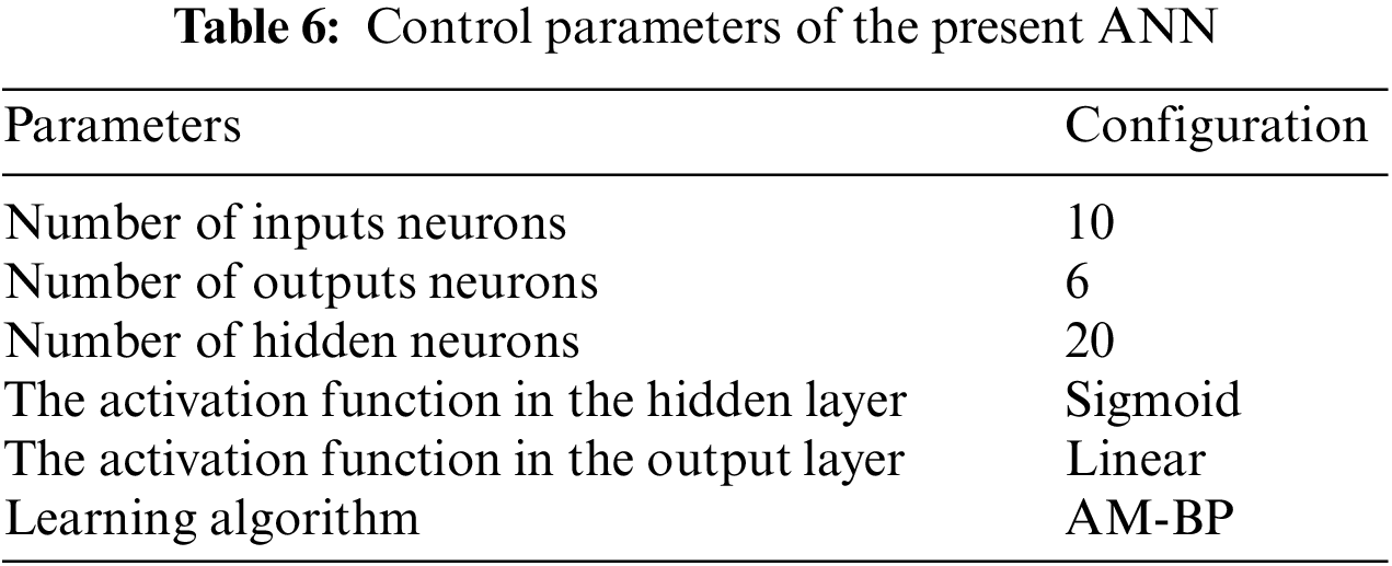
During flood prediction, ANN is fed ten significant meteorological factors detected by IoT sensors. Also, the ANN model includes 20 hidden neurons. The proposed ANN model is shown in Fig. 4. Depending on how much rain is expected to fall in a day or an hour, five types of precipitation are predicted: violent rain, extremely heavy rain, heavy rain, moderate rain, light rain, and no precipitation. The classification of rainfall is detailed in Table 4.

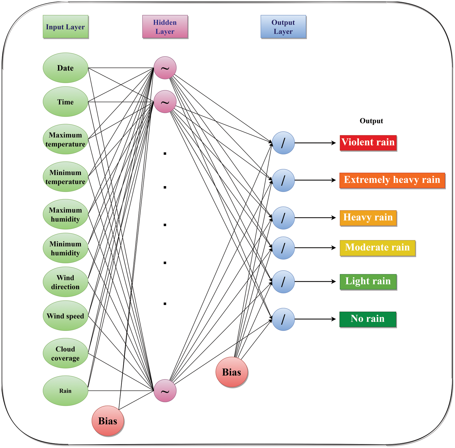
Figure 4: Proposed ANN model for predicting flood events

2.7 Training Optimization

Unlike programming languages, neural networks solve problems through learning. Learning is achieved by neural networks through the model training process [46]. To ensure the success of the training, different parts of the data must be examined. The training efficiency of neural network models is dependent on the data and the learning algorithm adopted [47,48]. Advanced learning algorithms effectively transfer intelligence to the ANN from historical facts or data. Typically, ANN models use the backpropagation (BP) algorithm as their learning algorithm [49]. BP attains the appropriate learning rate (learning rate is a small positive integer. It indicates the rate at which the neuron updates its learned knowledge) by decreasing or increasing the learning rate in both the forward and reverse directions [50]. The traditional BP algorithm performs better when the size of the data set is modest. However, as the size of the data set grows, achieving the ideal learning rate takes a large amount of time. To address this problem, the traditional BP algorithm has been hybridized in this study. Formula (10) is used to adjust the weight in the conventional backpropagation procedure. The weight increase is represented by w(t+1)the learning rate by η and the total error by d(E).

w(t+1)=wt−ηd(E)d(w1)(10)

In order to accelerate the training process of backpropagation, adaptive momentum (AM) and backpropagation (BP) have been integrated into this study (BP-AM). The parameter selection and weight-updating procedure of an ANN can be accomplished in a highly efficient manner using adaptive momentum. The following equation depicts the BP-AM weight-updating procedure:

Δw(n)=−ηEw(w(n))+α(n)Δw(n−1) n=0,1,…(11)

In the previous equation, η represents the learning rate, α denotes adaptive momentum, and n is the number of iterations for weight update. The adaptive momentum α is updated in the following way:

αi(n)={αηEw(w(n)).Δwn−1||Δw(n−1)||20, ifEw(w(w(n)).Δw(n−1)<0(12)

In the above equation αi(n)=α1,α2,α3,…,αn. BP-AM self-adjusts continuously by calculating the present weighting coefficients by the most recent weighting coefficients. If the AM values are less than zero, a positive integer is assigned to them in order to speed learning by updating momentum. Otherwise, the AM is set to zero to keep the error downward. In Algorithm 1, the processing steps of the proposed BP-AM are described.

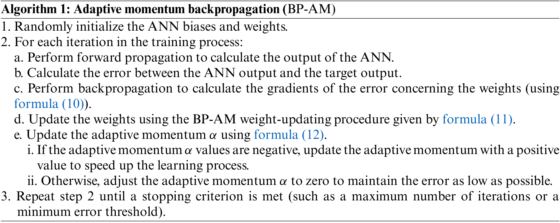
The BP-AM algorithm integrates adaptive momentum into the traditional backpropagation process to improve the efficiency of hyperparameter tuning in ANNs. The weights are updated using both the current gradients and the previous weight changes, with the adaptive momentum term providing a self-adjusting mechanism to accelerate convergence.

2.8 Flood Forecasting Using Presentation Layer

In this research, an Artificial Neural Network (ANN) is employed to predict the amount of rainfall in a specific study area, which serves as the basis for issuing flood warnings 24 h in advance. This proactive approach enables residents and authorities to take necessary precautions and minimize potential damage. The flood warning system is disseminated through various channels, including a mobile app, social media, and a dedicated website. Key features of this system are:

1.    Rainfall Prediction: The ANN model predicts the amount of rainfall in the next 24 h, giving residents and authorities ample time to prepare for potential flooding.

2.    Flood Map: The flood map illustrates the areas expected to be affected by flooding, enabling individuals to visualize and understand the extent of the potential flood.

3.    Flood Zones: The system identifies different flood zones, categorizing areas by their risk level. This information is crucial for evacuation planning and resource allocation.

4.    Safer Zones: The system highlights safer zones within the study area, providing guidance for evacuation routes and temporary shelter locations.

5.    Lightweight Design: The web portal is designed to be lightweight and accessible even in remote locations with limited network coverage, ensuring that warnings reach all potentially affected individuals.

6.    Emergency Communication Feature: The website includes a feature to facilitate communication between residents and the government’s disaster management team. This allows users to report damage, request assistance, or share information about the emergency.

The process flow of disaster management is shown in Fig. 5.

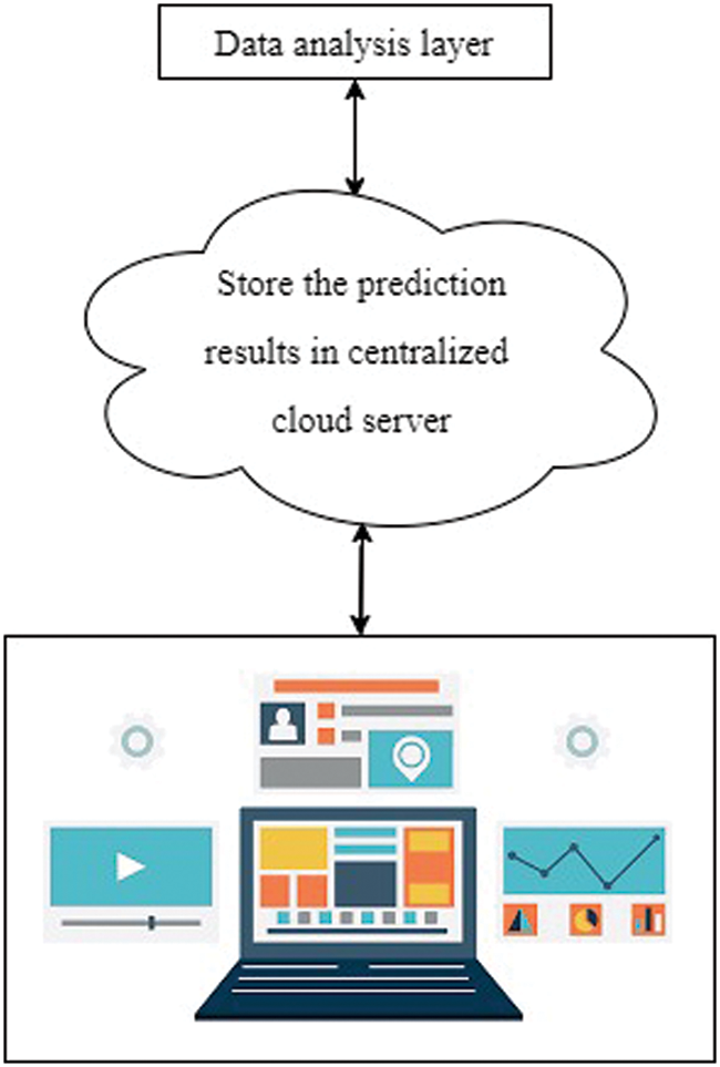
Figure 5: Visual representation of the presentation layer workflow

3  Results and Discussion

3.1 System Details

The proposed flood early warning system was implemented with the following computational hardware and software API. A desktop with the following specifications is used: 11th Gen Intel® CoreTM i5-11260H (12 MB cache, 6 cores, 12 threads, up to 4.40 GHz Turbo), NVIDIA GeForce RTX 3050, 4 GB GDDR6, 16 GB, 2 × 8 GB, DDR4, 3200 MHz and 512 GB, PCIe NVMe, SSD. The prediction model is developed using Python 3.7, TensorFlow, PyTorch, sci-learn, and Windows 10 as the operating system.

3.2 Dataset Analysis

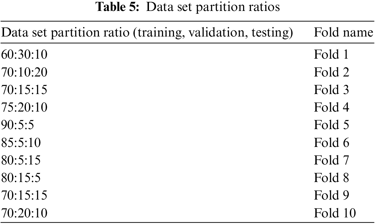
Training loss in ANN is an incorrect prediction caused by not selecting the most suitable features from labeled data using weights and bias. When an ANN model’s prediction is perfect, the loss is zero; otherwise, it is more than one. This section analyses the training effectiveness of the proposed flood prediction model. For this, the most prevalent accuracy metrics are Mean Absolute Error (MAE), Mean Square Error (MSE), and Root Mean Square Error (RMSE) are used. Formulas (8)–(10) are used to calculate these error evaluation procedures. When there are fewer errors, the amount of information lost during training is minimal. The data of the training set, testing set, and validation set are separated into multiple sizes, training, testing, and validation are performed and the average values are obtained to give a more trustworthy comparison. Table 5 lists the various partition ratios for data sets.

Absolute error is the error in the total number of observations (Total absolute error = total observations − actual). The following formula is used to calculate the MAE, which is the average absolute error value:

MAE=1N∑i=1N|yi−yi^|(13)

MSE is defined as the average square difference between observed weather data and predicted results.

MSE=1N∑i=1N|yi−yi^|2(14)

The RMSE returns the standard deviation of the difference between the observed data and estimation data of the weather forecast model.

RSME=1N∑i=1N|yi−yi^|2(15)

For experimental analysis, both the traditional BP algorithm and an AM-BP algorithm are utilized. The experiment’s configuration is listed in Table 6.

The comparison of the MAE, MSE, and RMSE between the traditional Backpropagation (BP) algorithm and the AM-BP algorithm are presented in Tables 7–9.

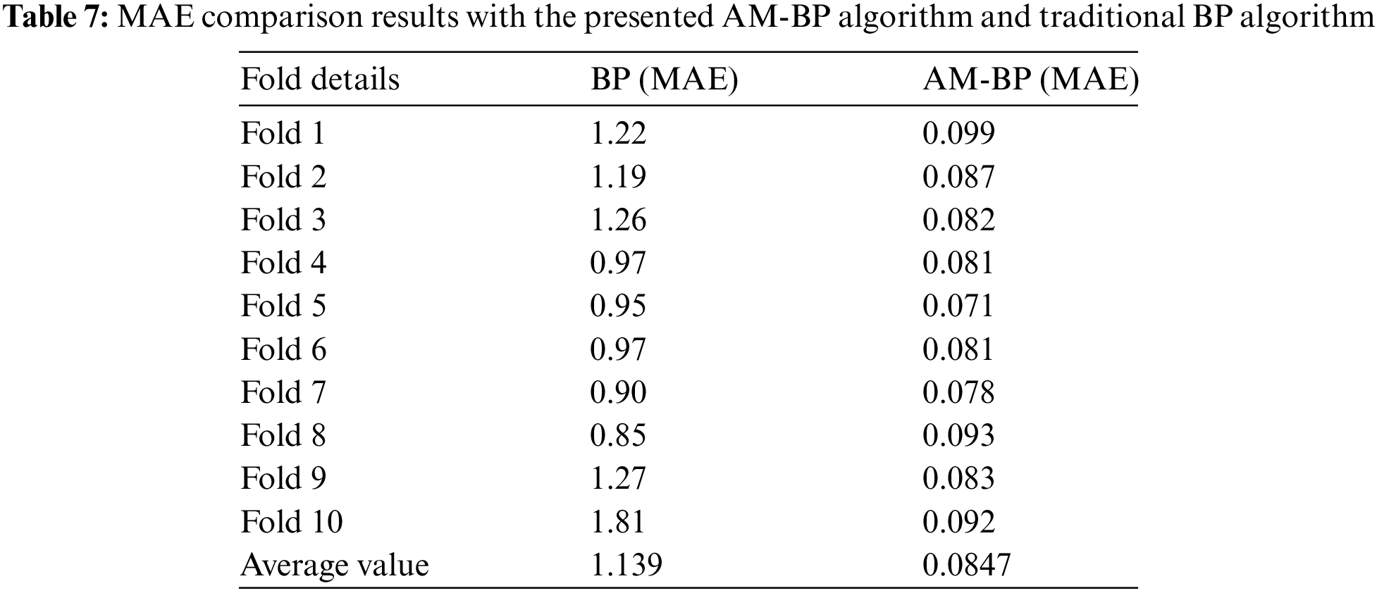
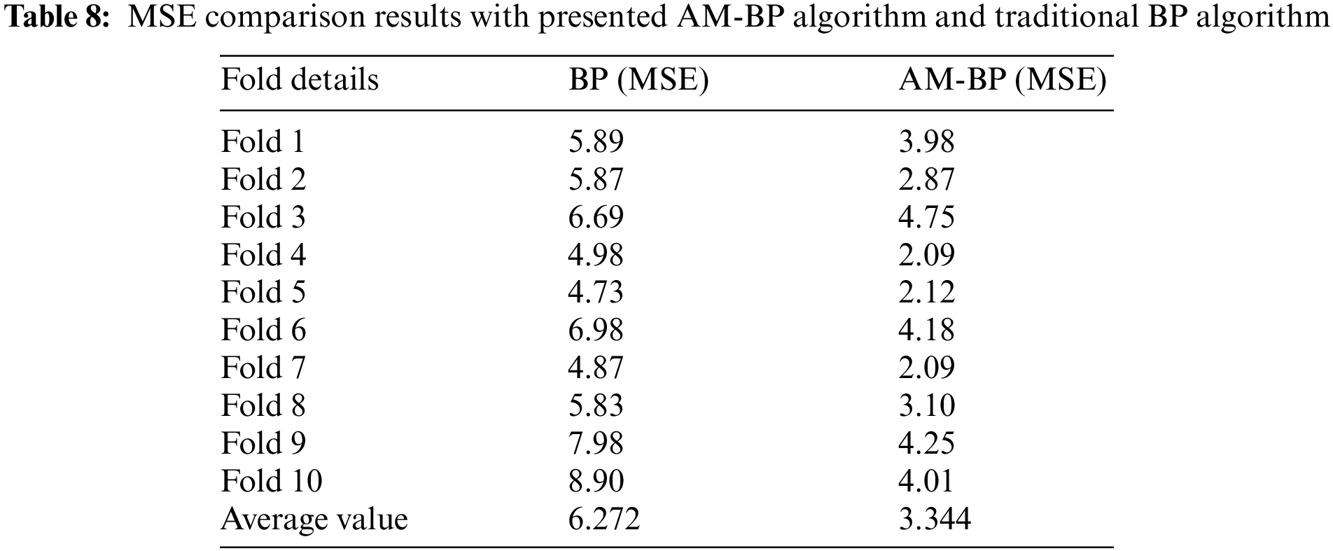
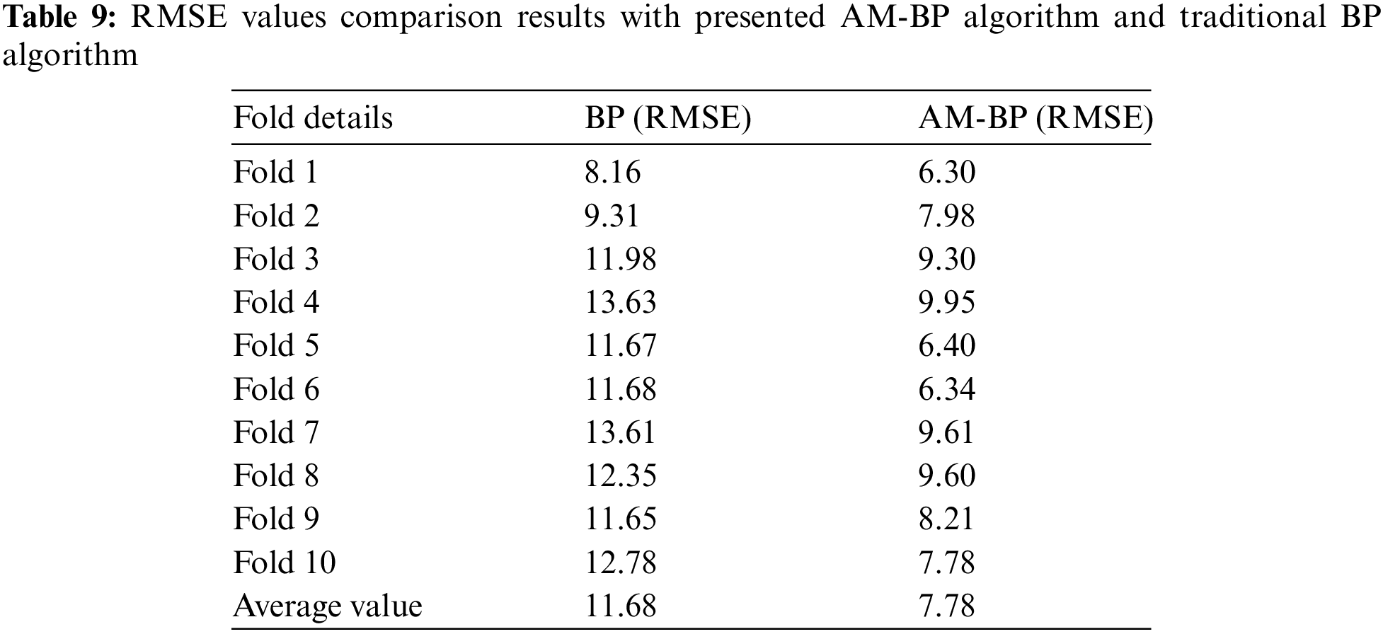
The MAE results in Table 7 show a significant reduction in error rate from an average of 1.139 in BP to 0.0847 in AM-BP. Similarly, the MSE results in Table 8 show an average of 6.272 in BP to 3.344 in AM-BP, illustrating a substantial improvement in error rates. RMSE results in Table 9 follow the same trend, reducing from an average of 11.68 in BP to 7.78 in AM-BP. These findings demonstrate that the AM-BP algorithm provides a much lower training error rate compared to the traditional BP algorithm. Therefore, the research shows that AM-BP can significantly improve the accuracy and efficiency of ANN-based flood prediction systems, making it a more reliable choice for handling heterogeneous weather data.

The prediction data from 2014 to 2019, as illustrated in Fig. 6, suggests that the proposed model’s output aligns closely with observed values, indicating a high level of accuracy.

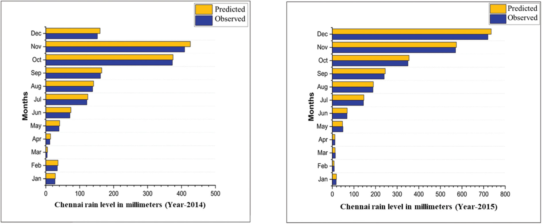
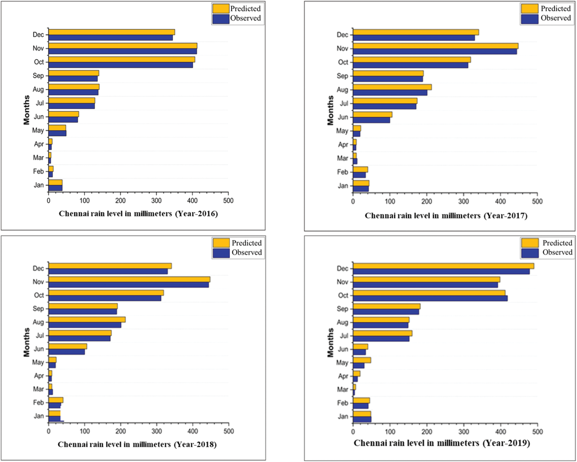
Figure 6: The results of the proposed method to predict precipitation in 2014–2019 before 24 h and the actual observations

3.3 Accuracy Analysis

Assessment based on the accuracy of the flood forecasting system and the machine learning models in existence is done using different measures of accuracy such as Total accuracy (A), Precision (P), Recall (R), and F1-Measure (F1). Using formulas (16)–(19) the accuracy of the proposed flood forecasting model is determined. These equations are dependent on True Negative flood prediction (TNFC), True Positive flood prediction (TPFC), False Negative flood prediction (FNFC) and False Positive flood prediction (FPFC).

A=TPFC+TNFCTPFC+TNFC+FPFC+FNFC(16)

P=TPFCTPFC+FPFC(17)

R=TPFCTPFC+FNFC(18)

F1=2(P×R)P+R(19)

Accuracy is one of the important features of the flood forecasting system. Many different outputs are achieved through false results. A comparison of the results of the accuracy of the proposed flood forecasting method and the existing methodologies are depicted in Fig. 7. The accuracy of the proposed flood forecasting system is achieved to be 96% accuracy, 96.4% F1-Measure, 97% Precision, and 95.9% recall. Fig. 7 demonstrates the AM-BP-based system’s high prediction accuracy and reliability. As depicted in Fig. 7, the AM-BP training procedure has improved the overall accuracy of the prediction model by 2% to 3%. These results show that the noise level of the training data is minimal and that the invention of the optimal training technique substantially enhances accuracy.

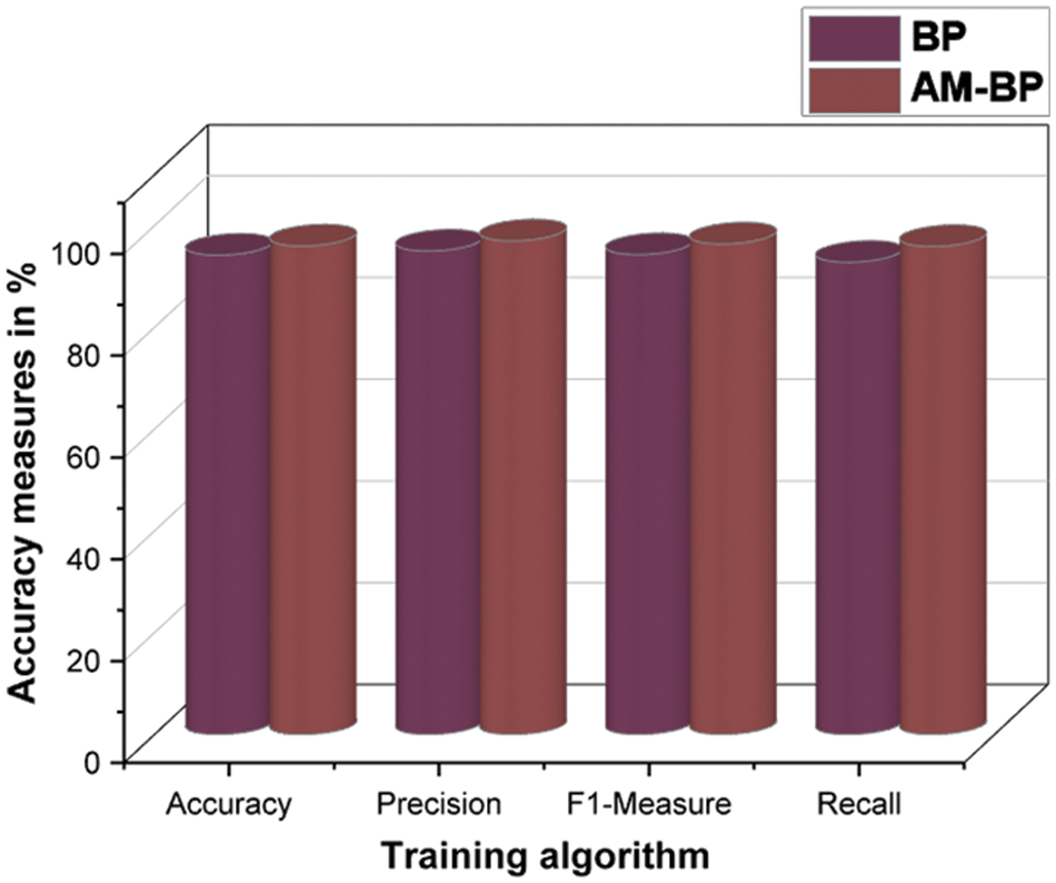
Figure 7: Accuracy comparison results

3.4 Accuracy Analysis with Existing Methods

In this section, we provide a comparative analysis of the proposed flood prediction method and the existing methods, namely Wan et al. [24], Puttinaovarat et al. [28], Dong et al. [32] and Khanna et al. [22]. The comparison is based on key performance metrics such as accuracy, recall, precision, and F1-score.

Fig. 8 shows the accuracy comparison with state-of-the-art flood prediction methods. In this comparative analysis, the proposed flood prediction method outperforms existing methods (Wan et al. [24], Puttinaovarat et al. [28], Dong et al. [32], and Khanna et al. [22]) across key performance metrics such as accuracy, recall, precision, and F1-score. The proposed method demonstrates superior performance in identifying true flood events, avoiding false alarms, and providing a balanced evaluation of the model’s effectiveness. The improved performance can be attributed to the novel techniques and features integrated into the proposed model. Further research and development could result in even more accurate and reliable flood prediction models, ultimately reducing the devastating impacts of floods on people, infrastructure, and the environment.

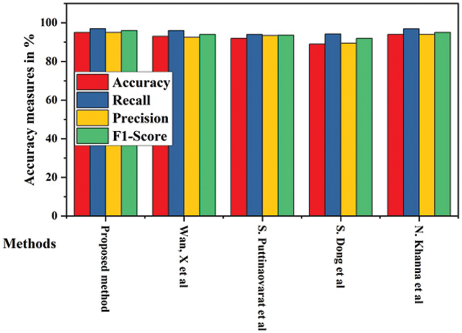
Figure 8: Accuracy comparison with state-of-the-art flood prediction methods

3.5 Regression Analysis

Regression analysis represents the relationship between the predicted and observed values. This determination coefficient represents the degree of relationship between the two factors. Regression analysis returns values between 1 and −1. Higher values closer to 1 suggest a greater degree of similarity, whereas lower values closer to −1 suggest a lower similarity. Regression values for the proposed forecasting model are calculated using formula (20).

R2=[n[∑i=1n(Fov∗Fpv)−(∑i=1nFov)(∑i=1nFpv)]]2[n∑i=1nFov2−(Fov)2]−[n∑i=1nFpv2−(Fpv)2](20)

In above equations Fov represents the observed values, Fpv represents the predicted values of the flood prediction model, Fov¯ represents the mean of the observed flood results, and n represents the total number of observations. R2 represents the regression values.

Fig. 9 depicts the model’s predicted chance of flooding based on regression analysis. This study employed test data from 2014 to 2019 for the implementation of a regression analysis. According to the figures, in most cases, the prediction results and the observed values are very close. This shows that the prediction efficiency of the proposed forecasting model is very similar to the real value. The right-side gradient line in the figure represents the severity of the flood, with the top red indicating high levels of rainfall and the bottom blue indicating low levels of rainfall.

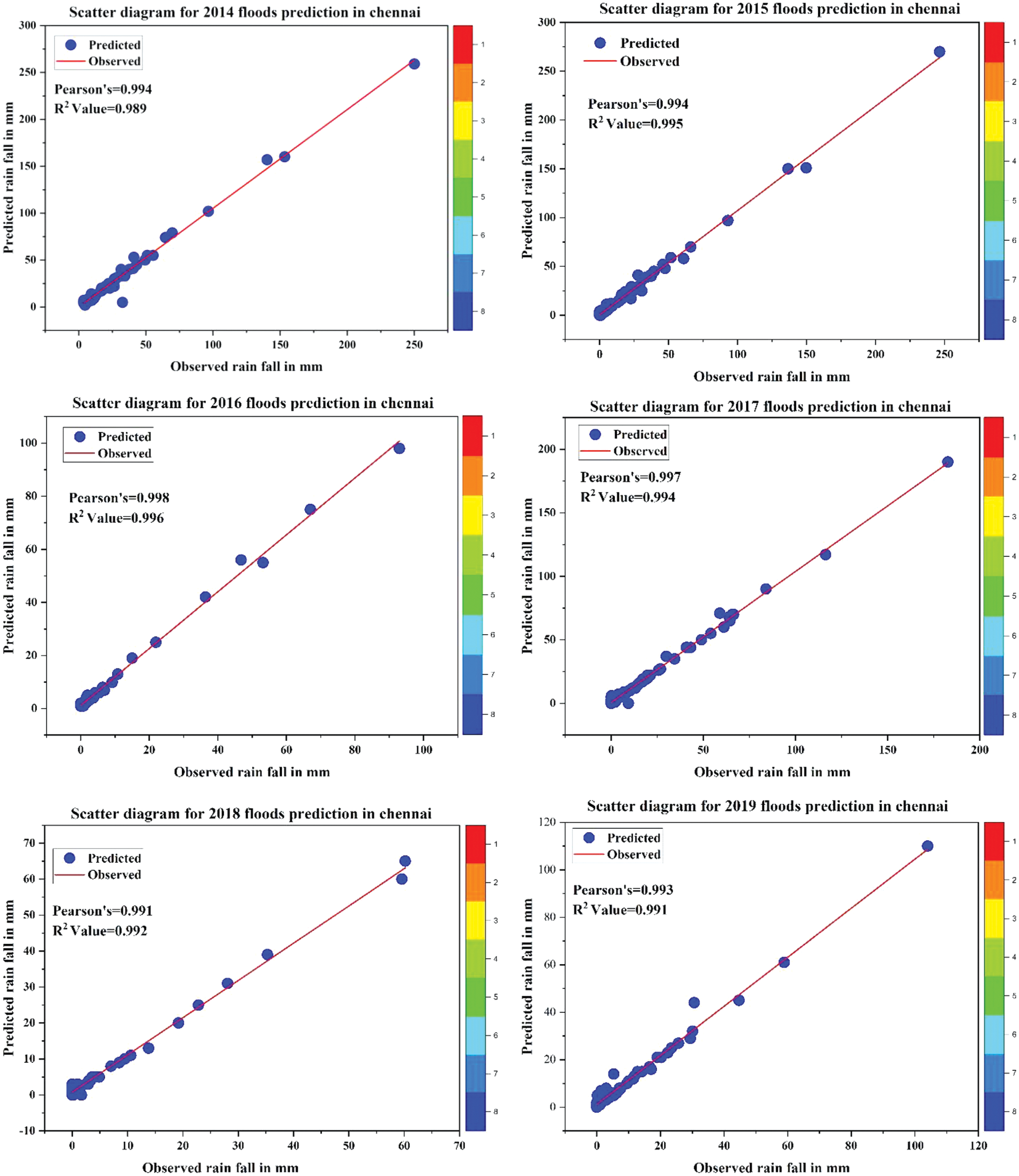
Figure 9: The chance of flooding in Chennai from 2014 to 2019 is based on regression analysis

3.6 Discussion

According to the United Nations, floods are responsible for an average of 240,000 deaths and 19 million displaced people per year. “Flood modeling” is the attempt to construct computerized representations of floods to simulate different possibilities and inform flood risk management. An efficient flood model must be able to predict the behavior of a flood, including the propagation, the impacts and extent of flooding, the risks involved, and how to respond in terms of prevention, early warning, and evacuation. Despite the development of numerous computerized flood prediction models, no model to date has been effective. In this study, IoT and AI were efficiently combined to create a successful flood prediction model. This innovative flood forecasting system features an integrated architecture with four layers. The bottom layer collects weather data for the prediction model using IoT sensors. High computational resources are needed to process the data because the volume of data being collected is always increasing. Consequently, a fog computing layer with high processing resources has been placed between the data analysis and weather monitoring layers in this research. It primarily supplies the necessary computing power for the prediction model. Next, the data analysis layer is added, which consists of three essential components. First, there is a module for data pre-processing to reduce noise in the weather data. PCA is utilized to minimize the dimension of the data. Second, correlation analysis has been performed to exclude irrelevant data from the flood prediction model. To forecast floods, ANN was utilized in this study.

Training is a crucial component of an AI model. When utilizing the most effective training algorithms, training loss can be drastically decreased. In this study, adaptive momentum is used to optimize the training procedure of the BP algorithm to minimize training loss. Experimental data suggest that its training errors are lower. According to the experimental results, the MAE = 0.0847, MSE = 3.344, and RMSE = 7.78 of the proposed AM-BP algorithm are significantly lower than those of the BP algorithm (MAE = 1.139, MSE = 6.272, and RMSE = 11.68). The comparison of MAE, MSE, and RMSE is summarized in Tables 7 to 9. The experimental results demonstrate that the suggested model can more accurately forecast the rain that will occur in the study area 24 h in advance. The predictions for the years 2014 to 2019 are depicted in Fig. 6. The predicted values of the proposed model and observed values are almost slimmer. In addition, comparisons and analyses of precision, F1-Measure, recall, and accuracy have been conducted. According to the results, the proposed method achieves 5% Precision, 2% F1-Measure, 5% recall, and 3% accuracy recall more than the existing methods.

Compared to prior research, the proposed AM-BP algorithm and MLCA for flood prediction and management offer several outstanding improvements and achievements. The AM-BP algorithm enhances the parameter tuning process of ANN, leading to better model accuracy and performance, addressing the limitations of prior research that suffered from suboptimal tuning processes. The MLCA’s hierarchical design provides a scalable and efficient solution for handling large volumes of weather data, overcoming the scalability issues faced by existing models in prior research.

By incorporating fog computing for local data processing and analysis, the MLCA reduces latency and improves responsiveness in real-time flood prediction applications, addressing limitations of prior research that struggled with high latency and reduced responsiveness. The MLCA leverages cloud computing for large-scale storage, processing, and advanced analytics, enabling more effective flood prediction and management compared to existing models in prior research that struggled with handling large-scale weather data.

Moreover, the proposed AM-BP algorithm and MLCA are designed to be more versatile, making them applicable to various flood scenarios and locations, addressing the limitations of prior research where models were designed for specific scenarios or locations and could not be easily adapted. In comparison to traditional BP algorithms, the proposed AM-BP algorithm demonstrates superior performance in terms of MAE, MSE, and RMSE as mentioned earlier. The significant improvements in these performance metrics can be attributed to the enhanced parameter tuning process in the AM-BP algorithm and the integration of the MLCA for flood prediction and management. These outstanding improvements and achievements demonstrate the potential of the proposed research to advance the field of flood prediction and management, providing more accurate, scalable, and efficient solutions for handling weather big data and real-time flood prediction applications.

In addition, as discussed in [51] and [52] for the past two decades, the Underwater Internet of Things (UIoT) is widely used for developing Industrial applications such as deep-sea monitoring, diver network monitoring, early warning system, etc., among that early prediction of tsunami is much necessary to protect human life from danger. In this case, the proposed AM-BP model can be used to predict the accuracy of a tsunami by deploying and frequent collection of data from the deep-sea environment.

4  Conclusion

In this paper, the proposed AM-BP model offers a promising solution for flood monitoring, management, and decision-making in IoT systems. By incorporating the adaptive momentum algorithm with the back propagation algorithm, the model demonstrates improved accuracy, speed, and generalization ability. The adaptive nature of the AM-BP model allows it to dynamically adjust the learning rate and momentum parameters during the training process, enabling faster convergence and better adaptation to different flood patterns and conditions. This enhances the model’s prediction accuracy and its ability to capture complex relationships in flood data. The experiments conducted using real-world flood data demonstrate that the adaptive momentum and back propagation model outperforms existing methods in terms of accuracy and efficiency. The model achieves high prediction accuracy, enabling timely and accurate flood warnings and management decisions. Furthermore, the adaptability of the model is a significant advantage for flood monitoring and management systems. As flood patterns and conditions can change over time, it is crucial for the model to continuously update itself with new data to make accurate predictions. The adaptive nature of the model allows it to learn and adjust its predictions based on the latest information, improving its effectiveness in flood monitoring and management.

Overall, the adaptive momentum and back propagation model presented in this study has the potential to significantly improve flood prediction and management. By providing accurate and timely predictions, the model can enhance preparedness and reduce damage in flood-prone areas. Further research and implementation of this model in real-world flood monitoring and management systems can lead to more effective and efficient flood management strategies. Experimental results demonstrate the superiority of the proposed AM-BP algorithm, achieving a 96% accuracy, 96.4% F1-Measure, 97% Precision, and 95.9% recall. These metrics illustrate the significant advancements compared to previous flood prediction models. In the future, the current methodology can be utilized in underwater networks by extending and adapting the proposed AB-BP learning algorithm to UIoT networks to improve prediction accuracy. Thus, a natural disaster caused by deep-sea environments such as tsunamis, undersea landslides, the deep-water fast wave, etc. can be predicted.

Acknowledgement: None.

Funding Statement: This work was supported by the Korea Polar Research Institute (KOPRI) grant funded by the Ministry of Oceans and Fisheries (KOPRI Project No. *PE22900).

Author Contributions: Conceptualization, J.T.; methodology, J.T., and D.R.K.M.; software, D.J.Y.; data curation, S.H.P.; writing—original draft preparation, J.T., and D.R.K.M.; writing—review and editing, S.H.P.; supervision, D.J.Y., and S.H.P.

Availability of Data and Materials: The data used in this paper can be requested from the authors upon request.

Conflicts of Interest: The authors declare that they have no conflicts of interest to report regarding the present study.

References

1. L. Landuyt, F. M. B. van Coillie, B. Vogels, J. Deweldeand and N. E. C. Verhoest, “Towards operational flood monitoring in Flanders using sentinel-1,” IEEE Journal of Selected Topics in Applied Earth Observations and Remote Sensing, vol. 14, pp. 11004–11018, 2021. [Google Scholar]

2. A. Zhai, G. Fan, X. Ding and G. Huang, “Regression tree ensemble rainfall–runoff forecasting model and its application to Xiangxi river, China,” Water, vol. 14, no. 3, pp. 364–368, 2022. [Google Scholar]

3. F. Xue, W. Gao, C. Yin, X. Chin and Z. Xia, “Flood monitoring by integrating normalized difference flood index and probability distribution of water bodies,” IEEE Journal of Selected Topics in Applied Earth Observations and Remote Sensing, vol. 15, pp. 4170–4179, 2022. [Google Scholar]

4. N. Akhtar, A. Rehman, M. Hussnain, S. Rohail, M. S. Missen et al., “Hierarchical coloured petri-net based multi-agent system for flood monitoring, prediction, and rescue (FMPR),” IEEE Access, vol. 7, pp. 180544–180557, 2019. [Google Scholar]

5. E. Munsaka, C. Mudavanhu and L. Sakala, “When disaster risk management systems fail: The case of Cyclone Idai in Chimanimani District, Zimbabwe,” International Journal of Disaster Risk Science, vol. 12, pp. 689–699, 2021. [Google Scholar]

6. P. Rai and V. Khawas, “Traditional knowledge system in disaster risk reduction: Exploration, acknowledgement and proposition,” Jamba, vol. 11, no. 1, pp. 484–498, 2019. [Google Scholar] [PubMed]

7. H. Zhang, S. Lee, Y. Lu, X. Yu and H. Lu, “A survey on big data technologies and their applications to the metaverse: Past, current and future,” Mathematics, vol. 11, no. 1, pp. 96–111, 2023. [Google Scholar]

8. T. Vasantha Kumaran, O. M. Murali and S. R. Senthamarai, “Chennai floods 2005, 2015: Vulnerability, risk and climate change,” in Urban Health Risk and Resilience in Asian Cities, Delhi, India: Springer, pp. 73–100, 2020. [Google Scholar]

9. N. Nithila Devi, B. Sridharan and S. N. Kuiry, “Impact of urban sprawl on future flooding in Chennai city, India,” Journal of Hydrology, vol. 574, pp. 486–496, 2019. [Google Scholar]

10. R. Krishnamurthi, A. Kumar, D. Gopinathan, A. Nayyar and B. Qureshi, “An overview of IoT sensor data processing, fusion, and analysis techniques,” Sensor, vol. 20, no. 21, pp. 6076, 2020. [Google Scholar] [PubMed]

11. C. Buratti, E. Ström, L. Feltrin, L. Clavier, G. Gardasevic et al., “IoT protocols, architectures, and applications,” Inclusive Radio Communications for 5G and Beyond, vol. 2021, pp. 187–220, 2021. [Google Scholar]

12. S. Kumar, P. Tiwari and M. Zymbler, “Internet of Things is a revolutionary approach for future technology enhancement: A review,” Journal of Big Data, vol. 6, pp. 111, 2019. [Google Scholar]

13. M. Esposito, L. Palma, A. Belli, L. Sabbatiniand and P. Pierleoni, “Recent advances in Internet of Things solutions for early warning systems: A review,” Sensors, vol. 22, no. 6, pp. 2124, 2022. [Google Scholar] [PubMed]

14. A. Mosavi, P. Ozturk and K. Chau, “Flood prediction using machine learning models: Literature review,” Water, vol. 10, no. 11, pp. 1536, 2018. [Google Scholar]

15. H. S. Munawar, A. W. A. Hammad and S. T. Waller, “Remote sensing methods for flood prediction: A review,” Sensors, vol. 22, no. 3, pp. 960, 2022. [Google Scholar] [PubMed]

16. C. Prakash, A. Barthwal and D. Acharya, “Floodwall: A real-time flash flood monitoring and forecasting system using IoT,” IEEE Sensors Journal, vol. 23, no. 1, pp. 787–799, 2023. [Google Scholar]

17. I. A. Ajah and H. F. Nweke,“Big data and business analytics: Trends, platforms, success factors and applications,” Big Data and Cognitive Computing, vol. 3, no. 2, pp. 32, 2019. [Google Scholar]

18. S. Sundaram, S. Devaraj and K. Yarrakula, “Modeling, mapping and analysis of urban floods in India—A review on geospatial methodologies,” Environmental Science and Pollution Research, vol. 48, pp. 67940–67956, 2021. [Google Scholar]

19. N. Khoirunisa, C. Ku and C. Liu, “A GIS-based artificial neural network model for flood susceptibility assessment,” International Journal of Environmental Research and Public Health, vol. 18, pp. 1072, 2021. [Google Scholar] [PubMed]

20. H. Zhu, J. Leandro and Q. Lin, “Optimization of artificial neural network (ANN) for maximum flood inundation forecasts,” Water, vol. 13, no. 16, pp. 2252, 2021. [Google Scholar]

21. F. Y. Dtissibe, A. A. A. Ari, C. Titouna, O. Thiareand and A. M. Gueroui, “Flood forecasting based on an artificial neural network scheme,” Natural Hazards, vol. 104, no. 2, pp. 1211–1237, 2020. [Google Scholar]

22. N. Khanna and M. Sachdeva, “OFFM-ANFIS analysis for flood prediction using mobile IoS, fog and cloud computing,” Cluster Computing, vol. 23, pp. 2659–2676, 2020. [Google Scholar]

23. M. Anbarasan, B. Muthu, C. B. Sivaparthiban, R. Sundarasekar, S. Kadry et al., “Detection of flood disaster system based on IoT, big data and convolutional deep neural network,” Computer Communications, vol. 150, pp. 150–157, 2020. [Google Scholar]

24. X. Wan, Q. Yang, P. Jiang and P. Zhong, “A hybrid model for real-time probabilistic flood forecasting using elman neural network with heterogeneity of error distributions,” Water Resources Management, vol. 33, no. 11, pp. 4027–4050, 2019. [Google Scholar]

25. J. A. Pollard, T. Spencer and S. Jude, “Big data approaches for coastal flood risk assessment and emergency response,” WIREs Climate Change, vol. 9, pp. 543, 2018. [Google Scholar]

26. S. Fang, L. D. Xu, Y. Zhu and J. Ahati, “An integrated system for regional environmental monitoring and management based on Internet of Things,” IEEE Transactions on Industrial Informatics, vol. 10, no. 2, pp. 1596–1605, 2014. [Google Scholar]

27. S. K. Sood, R. Sandhu, K. Singla and V. Chang, “IoT, big data and HPC based smart flood management framework,” Sustainable Computing: Informatics and Systems, vol. 20, pp. 102–117, 2018. [Google Scholar]

28. S. Puttinaovarat and P. Horkaew, “Flood forecasting system based on integrated big and crowdsource data by using machine learning techniques,” IEEE Access, vol. 8, pp. 5885–5905, 2020. [Google Scholar]

29. L. Hua, X. Wan, X. Wang, F. Zhao, P. Zhong et al., “Floodwater utilization based on reservoir pre-release strategy considering the worst-case scenario,” Water, vol. 12, no. 3, pp. 892–911, 2020. [Google Scholar]

30. C. Chen, Q. Hui, W. Xie, S. Wan, Y. Zhou et al., “Convolutional neural networks for forecasting flood process in Internet-of-Things enabled smart city,” Computer Networks, vol. 186, pp. 107744, 2021. [Google Scholar]

31. W. Dai and Z. Cai, “Predicting coastal urban floods using artificial neural network: The case study of Macau, China,” Applied Water Science, vol. 11, pp. 161, 2021. [Google Scholar]

32. S. Dong, T. Yu, H. Farahmand and A. Mostafavi, “A hybrid deep learning model for predictive flood warning and situation awareness using channel network sensors data,” Computer-Aided Civil and Sensor Data, vol. 2, pp. 9201–9218, 2020. [Google Scholar]

33. W. Hu, T. Chen and S. L. Shah, “Detection of frequent alarm patterns in industrial alarm floods using itemset mining methods,” IEEE Transactions on Industrial Electronics, vol. 65, no. 9, pp. 7290–7300, 2018. [Google Scholar]

34. I. H. Sarker, “Data science and analytics: An overview from data-driven smart computing, decision-making and applications perspective,” SN Computer Science, vol. 2, pp. 377, 2021. [Google Scholar] [PubMed]

35. V. Sebestyén, T. Czvetko and J. Abonyi, “The applicability of big data in climate change research: The importance of system of systems thinking,” Frontiers in Environmental Science, vol. 9, pp. 619092, 2021. [Google Scholar]

36. H. Zhou, H. Ren, P. Royar, H. Hou and X. Yu, “Big data analytics for long-term meteorological observations at hanford site,” Atmosphere, vol. 13, no. 1, pp. 136, 2022. [Google Scholar]

37. W. Xu, J. Chen, J. Zhang, L. Xiong and H. Chen, “A framework of integrating heterogeneous data sources for monthly streamflow prediction using a state-of-the-art deep learning model,” Journal of Hydrology, vol. 614, no. 2, pp. 128599, 2022. [Google Scholar]

38. P. F. Kuo, T. E. Huang and I. G. B. Putra, “Comparing kriging estimators using weather station data and local greenhouse sensors,” Sensors, vol. 21, no. 5, pp. 1853, 2021. [Google Scholar] [PubMed]

39. M. H. Esfe, R. Esmaily, M. K. Khabaz, A. Alizadeh, M. Pirmoradian et al., “A novel integrated model to improve the dynamic viscosity of MWCNT-Al2O3 (40:60)/Oil 5W50 hybrid nnano-lubricant using artificial neural networks (ANNs),” Tribology International, vol. 178, pp. 108086, 2023. [Google Scholar]

40. M. Yang, W. He, Z. Zhang, Y. Xu, H. Yang et al., “An efficient storage and service method for multi-source merging meteorological big data in cloud environment,” EURASIP Journal on Wireless Communicationsand Networking, vol. 2019, pp. 241, 2019. [Google Scholar]

41. S. Xie, W. Wu, S. Mooser, Q. J. Wang, R. Nathan et al., “Artificial neural networkbased hybrid modeling approach for flood inundation modeling,” Journal of Hydrology, vol. 592, pp. 125605, 2021. [Google Scholar]

42. D. M. Ahmed, M. M. Hassan and R. J. Mstafa, “A review on deep sequential models for forecasting time series data,” Applied Computational Intelligence and Soft Computing, vol. 2022, pp. 19, 2022. [Google Scholar]

43. P. Kuppusamy, N. M. J. Kumari, W. Y. Alghamdi, H. Alyami, R. Ramalingam et al., “Job scheduling problem in fog-cloud-based environment using reinforced social spider optimization,” Journal of Cloud Computing: Advances, Systems and Applications, vol. 11, pp. 99, 2022. [Google Scholar]

44. J. Zou, Y. Han and S. S. So, “Overview of artificial neural networks,” Artificial Neural Networks, vol. 3, pp. 14–22, 2008. [Google Scholar]

45. M. Mohseni-Dargah, Z. Falahati, B. Dabirmanesh, P. Nasrollahi and K. Khajeh, “Machine learning in surface plasmon resonance for environmental monitoring,” Artificial Intelligence and Data Science in Environmental Sensing, vol. 2022, pp. 269–298, 2022. [Google Scholar]

46. C. Zhu, O. D. Samuel, N. Elboughdiri, M. Abbas, C. A. Saleel et al., “Artificial neural networks vs. gene expression programming for predicting emission & engine efficiency of SI operated on blends of gasoline-methanol-hydrogen fuel,” Case Studies in Thermal Engineering, vol. 49, no. 7, pp. 103109, 2023. [Google Scholar]

47. L. Cavallaro, O. Bagdasar, P. de Meo, G. Fiumara and A. Liotta, “Artificial neural networks training acceleration through network science strategies,” Soft Computing, vol. 24, no. 23, pp. 17787–17795, 2020. [Google Scholar]

48. C. Janiesch, P. Zschech and K. Heinrich, “Machine learning and deep learning,” Electron Markets, vol. 31, no. 4, pp. 685–695, 2021. [Google Scholar]

49. W. Sun, X. Wang and B. Tan, “Multi-step wind speed forecasting based on a hybrid decomposition technique and an improved back-propagation neural network,” Environmental Science Pollution Research, vol. 29, no. 33, pp. 49684–49699, 2022. [Google Scholar] [PubMed]

50. O. I. Abiodun, “Comprehensive review of artificial neural network applications to pattern recognition,” IEEE Access, vol. 7, pp. 158820–158846, 2019. [Google Scholar]

51. N. Victor, R. Chengoden, M. Alazab, S. Bhattacharya, S. Magnusson et al., “Federated learning for IoUT: Concepts, applications, challenges and future directions,” IEEE Internet of Things Magazine, vol. 5, no. 4, pp. 36–41, 2022. [Google Scholar]

52. S. Bhattacharya, N. Victor, R. Chengoden, M. Ramalingam, G. Selvi et al., “Blockchain for internet of underwater things: State-of-the-art, applications, challenges, and future directions,” Sustainability, vol. 14, no. 23, pp. 15659, 2022. [Google Scholar]