Recognizing Breast Cancer Using Edge-Weighted Texture Features of Histopathology Images

1  Introduction

Cancer incidence continues to rise, making it the top cause of death worldwide. The fact that breast cancer is the second most common disease in women makes it an important global health concern. There is a worldwide problem with breast cancer. By the year 2020, the World Health Organization predicted there would be an additional 2.3 million instances of breast cancer worldwide. In terms of female fatalities, breast cancer ranks sixth. There appears to be no consistent breast cancer mortality rate. Breast cancer rates are higher in wealthy countries than in less developed ones because of differences in nutrition, exercise, and reproduction rates. With an estimated 284,200 new cases in 2021 and 44,130 deaths, breast cancer is the leading cause of death among American women [1]. Breast cancer mortality rates in developed nations have been falling over the past few decades as the disease has been better diagnosed and treated. Despite this, breast cancer remains a major health concern worldwide, particularly in underdeveloped countries with scarce diagnostic and therapeutic options. Mammography and other imaging screening should begin for women of average risk at 40 since breast cancer survival rates are increased via early identification. Increased frequency of testing for breast cancer may be necessary for women with a family history or other risk factors. Early breast cancer staging is essential to increase the chances of successful therapy and rapid recovery. Accurate diagnosis and staging, which permits prompt intervention with surgery, radiation therapy, chemotherapy, or any combination thereof, are often the consequence of several factors contributing to improved treatment outcomes.

Technology has made cancer detection more sensitive and accurate. X-rays, Magnetic Resonance Imaging (MRI), Computed Tomography (CT), ultrasound, biopsy, and lab testing are used to identify cancer. The biopsy includes evaluating a small tissue sample from the suspected location under a microscope for cancer cells. Blood and tumor marker testing can also detect cancer cells or cancer-related chemicals. Conventional cancer detection technologies have drawbacks. Imaging may miss tiny tumors, and biopsy and laboratory testing may give erroneous positive or negative results. Liquid biopsy can detect cancer cells or DNA fragments in the blood. This non-invasive approach may diagnose cancer earlier and assess therapy response. Common machine learning methods, including Support Vector Machines (SVM), Random Forests, and K-Nearest Neighbors (KNN), have all been used for breast cancer classification [2,3]. These algorithms’ statistical and mathematical foundations allow for extracting useful insights from seemingly unconnected information. However, feature engineering, the process of selecting and extracting pertinent qualities from the data, is typically required when using traditional machine learning approaches. It might be lengthy when dealing with extensive data like histopathology images. Automating various domains using machine learning and deep learning is easy. Applications range from image forgery recognition and smart city infrastructure to medical care and agricultural water distribution [4–7].

Classifying breast cancer histopathology images using deep learning models and other machine learning approaches is an active study area. Deep learning models like Convolutional Neural Networks (CNNs) have recently been used to classify breast cancer [8–10]. For instance, the effectiveness of SVM, KNN, and CNN models was evaluated on breast cancer histopathological images. The CNN model had the greatest accuracy (95.29%) of all the machine-learning methods. An interesting case in point is the classification of breast cancer using histopathology images, where different deep-learning models were compared, and the best model achieved an accuracy of 97.3% [11–15]. Combining histopathology images with a cutting-edge deep learning model called Deep Attention Ensemble Network (DAEN) [14] further demonstrates the superiority of deep learning models over conventional machine learning algorithms for breast cancer classification. Several papers have investigated the feasibility of using machine learning on histology images to categorize breast cancer better. Classifying breast cancer histopathology images using a combination of a support vector machine and a random forest resulted in an accuracy of 84.23 percent. Several machine learning models, including SVMs, KNNs, random forests, and CNNs, were tested and compared for their ability to classify breast cancer histology. Compared to the other approaches, CNN had the highest accuracy (96.8%) [15].

Classifying cancerous images using machine learning has been the subject of numerous studies. When contrasted to more conventional inspection techniques that use image processing and classification algorithms, however, it is determined that these methods require refinement. First, there is a significant gender gap in the data made public through competitions and other sources. Furthermore, studies have yet to focus on analyzing a combined dataset consisting of all magnification levels, even though most research has focused on analyzing histopathology images either on a single magnification or separately on several magnification levels. Second, the current breast cancer classification methods have poor performance on the best classification algorithms since they rely on statistical and textural elements of an image to make their classifications.

The findings of this study combined wavelet transformation with Extreme Gradient Boosting (XGBOOST) [16] to develop a technique for distinguishing between benign and malignant cancers. This study offers a scale-invariant strategy for labeling images as benign or malignant, regardless of their size, shape, or resolution. The suggested method classifies cancer as benign or malignant using the BreakHis 1.0 [17] dataset comprising four types of magnification levels. Important sub-sections include the preprocessing stage, during which images from various databases with varying types, sizes, and dimensions are input and converted into YCBCR channels, and the feature extraction and concatenation stages. The final step involves providing features to XGBOOST to classify them and developing a model for use by image forensic specialists.

Some crucial findings from the study are as follows:

1.    Even though there are many more benign images than malignant ones, Synthetic Minority Oversampling Technique (SMOTE) has been utilized to balance the dataset so that more useful insights can be gleaned from it using the BreakHis 1.0 dataset.

2.    The images are classified as benign or malignant using XGBOOST, and texture features are extracted using Wavelet transformation.

3.    If a method maintains its effectiveness regardless of the size of the image, it is said to be scale-invariant. Therefore, the scale invariance of the planned method is evaluated using images of varied sizes, shapes, and types.

The remainder of this article is organized in terms of time: Section 2 details the pertinent studies on breast cancer detection techniques. Section 3 provides a high-level overview of the steps involved in the proposed methodology, including preprocessing, feature extraction, and classification. The experimental data sets are discussed here as well. Section 4 presents experimental results and a discussion of the proposed design. Results from computations using the proposed architecture are tabulated and illustrated. The report finishes with a discussion of the results and recommendations for future study in Section 5.

2  Literature Review

Breast cancer is a serious global public health issue that profoundly impacts patient outcomes and healthcare systems. Early identification and accurate breast cancer diagnosis were crucial for patients to have a greater survival rate and pay less for medical care. Recently, machine learning algorithms have shown enormous promise in identifying and classifying breast cancer using images from histopathology. This literature review includes the most up-to-date findings on the limitations of machine learning algorithms for breast cancer classification.

Breast cancer grading using deep learning was created by Wetstein et al. [18] and tested using whole-slide histopathology images. The algorithm outperformed human pathologists at identifying low and intermediate tumor stages, achieving an accuracy rate of 80% and a Cohen’s Kappa of 0.59. The work highlighted the possibility of deep learning-based models for automating breast cancer grading on whole-slide images, which is important since accurate and consistent grading improves patient outcomes. To determine the most common and productive training-testing ratios for histological image recognition, Wakili et al. [19] quickly analyzed deep-learning-based models. A training-to-testing ratio of 80/20 was shown to yield the highest accuracy. DenTnet, a new method built on transfer learning and DenseNet, was also created by the authors to address the limitations of prior methods. DenTnet achieved up to 99.28% accuracy on the BreaKHis dataset, outperforming leading deep learning algorithms in computing performance and generalizability. DenTnet allowed us to use fewer computational resources while maintaining our previous feature distribution. DenTnet tested only whole slide images but it was not tested on different resolutions.

Kadhim et al. [20] used the Histogram of Gradients (HOG) feature extractor to quantify invasive ductal carcinoma histopathology images. Area Under Curve (AUC), F1 score, specificity, accuracy, sensitivity, and precision were used to evaluate the algorithms’ performance. With more than 100 images, the algorithms struggled to keep up with the data. Deep learning could help get over this limitation. By reducing the scope for human error, machine learning (ML) can potentially improve breast cancer detection and survival rates. Zhang et al. [21] developed BDR-CNN-GCN to detect breast cancer in mammograms better. When a convolutional graph network (GCN) and a CNN are combined with batch normalization (BN), dropout (DO), and rank-based stochastic pooling (RSP), performance is improved. After being evaluated ten times on the breast miniMIAS dataset, the model has a sensitivity of 96.202 percent, a specificity of 96.002 percent, and an accuracy of 96.101 percent. Compared to 15 state-of-the-art breast cancer detection approaches and five neural network models, BDR-CNN-GCN achieves better results regarding data augmentation and identifying malignant breast masses.

The sliding window method for extracting features from Local Binary Patterns (LBP) characteristics was developed by Alqudah et al. [22]. Overall, the proposed method achieves high accuracy, sensitivity, and specificity, with a 91.12% rate of correct predictions, an 85.22% rate of correct positive predictions, and a 94.01% rate of correct negative predictions. In comparison to other studies in the literature, these outcomes excel. More information can be extracted using the suggested method, and other machine-learning strategies can be compared. The technique can potentially enhance breast cancer diagnosis and histological tissue localization. Clementet et al.’s support vector machine classifier and four DCNN versions classified breast cancer histology images into eight categories [23]. A deep convolutional neural network (DCNN) was used to analyze images at many resolutions and produce a highly predictive multi-scale pooling image feature representation (MPIFR), which was then used by SVM to classify the images. Since it offers a fresh approach to reliably identifying various breast cancer subtypes, the proposed MPIFR technology may greatly enhance patient outcomes and breast cancer screening. Using the BreakHis histopathological breast cancer image dataset, we show a precision of 98.45 percent, a sensitivity of 97.48 percent, and an accuracy of 97.77 percent.

The MPIFR method can improve the precision of breast cancer diagnosis and patients’ health. Seo et al. [24] created a deep convolutional neural network (DCNN) that performs exceptionally well in classifying breast cancer. On the BreakHis topology BC image dataset, the ensemble model achieved higher accuracy (97.77%), sensitivity (97.48%), and precision (98.45%) than the prior state-of-the-art and an entire set of DCNN baseline models. To separate cells with and without nuclei, Saturi et al. [25] introduced a superpixel-clustering strategy based on optimization. The proposed method outperformed prior studies, resulting in an 8%–9% increase in classification accuracy for identifying breast cancer. The improved segmentation results result from the method’s advantages, which include searching for global optimization and using parallel computing.

In [26], Hao et al. suggested a deep semantic and Grey Level Co-Occurrence Matrix (GLCM) based technique to image recognition in breast cancer histopathology. The suggested method outperforms the baseline models in Magnification Specific (MSB) and Magnification Independent (MIB) classification, with recognition accuracies of 96.75%, 95.21%, 96.57%, and 93.15% at magnifications of 40, 100, 200, and 400, respectively, and 96.33%, 95.26%, 96.09%, and 92.99% at the patient level. At the individual patient level, MIB classification accuracy was 95.56 percent, and at the individual image level, it was 95.54%. The suggested method’s accuracy is comparable to current best practices in recognition. Rehman et al. [27] proposed a neural network-based, reduced feature vector-and-machine learning framework to distinguish between mitotic and non-mitotic cells. The suggested method could accurately capture cell texture, allowing for the creation of efficiently reduced feature vectors to identify malignant cells. The proposed technique used ensemble learning with weighted attributes to improve model performance. The proposed method for recognizing mitotic cells outperforms state-of-the-art methods on the MITOS-12, AMIDA-13, MITOS-14, and TUPAC16 datasets. Different feature extraction methods (Hu moment, Haralick textures, and color histogram) created by Joseph et al. allowed for successful multi-classification of breast cancer cases on the BreakHis dataset. Histological images supported the multi-classification strategy recommended for breast cancer, which outperformed the majority of other investigations. Histopathological images at 40X, 100X, 200X, and 400X magnifications were classified with accuracies of 97.87%, 97.60%, 96.10%, and 96.84% using the proposed method [28].

Increasing patient survival rates and decreasing healthcare costs require early identification and accurate breast cancer diagnosis. Machine learning algorithms have shown potential in detecting and classifying breast cancer using histopathology images. Recent studies have investigated many approaches to grading breast cancer, including superpixel clustering algorithms, sliding window feature extraction methods, and deep learning-based models. These studies have shown that the proposed methods are superior to alternative procedures concerning accuracy, sensitivity, and specificity, all contributing to improved breast cancer detection. These procedures have the potential to enhance patient outcomes while decreasing healthcare costs. Among the many limitations and challenges that must be surmounted are the interpretability of machine learning models and the requirement for additional labeled data.

3  Material and Methods

The whole-slide classification machine learning pipeline has great potential for use in the detection and treatment of breast cancer. We analyze high-resolution images from databases like BreakHis to classify slides as cancerous or benign. The images were converted to YCBCR for optimal texture feature extraction. After the first image processing, texture features were retrieved using wavelet coefficients. A binary classifier was then given the extracted features. Any algorithm distinguishing between cancerous and noncancerous slides can be the classifier. The dataset must be resampled before classification can begin. Oversampling using SMOTE analysis is being used to rectify this inequitable data set. XGBOOST is handling classification in this investigation. The pipeline then reports the classification results. Metrics like accuracy, precision, recall, and F1 score may be included in the report. These indicators can be used to assess the pipeline’s efficiency and adjust the various stages accordingly. The pipeline consists of four phases: preprocessing, feature extraction, classification, and result reporting Fig. 1.

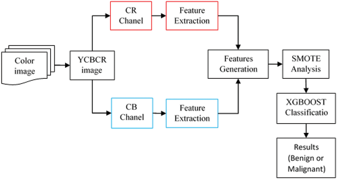
Figure 1: Workflow of proposed breast cancer classification method

3.1 Datasets

This section describes the data collecting and preprocessing methods used to train and assess the models employed in the machine learning pipeline. Table 1 summarizes the features of BreakHis 1.0. The BreakHis 1.0 database contains images of breast cancer tissue samples. The images are separated into two categories: normal and malignant. The magnifications used to capture these images range from 40X to 400X. The total number of images is 3,995, with 1,995 showing malignant growths and 2,000 showing noncancerous ones. Each image is a Portable Network Graphics (PNG) file of 7004603 pixels. The BreakHis dataset’s wide range of image sizes makes it perfect for teaching recognition models to scale.

Breast histopathology images from the BreakHis 1.0 dataset. The dataset includes 9,109 microscopic images of both healthy and malignant breast tissue. These images were captured at four magnifications (40X, 100X, 200X, and 400X) with two distinct staining procedures (hematoxylin, eosin, and picrosirius red). Studies have used the BreakHis 1.0 dataset to train and evaluate algorithms for breast cancer diagnosis and prognosis. Thus, we have developed deep learning models for automatically classifying breast histopathology images, which has greatly improved the progress of CAD systems [29]. Fig. 2 displays a few examples of the experimental database’s image content.

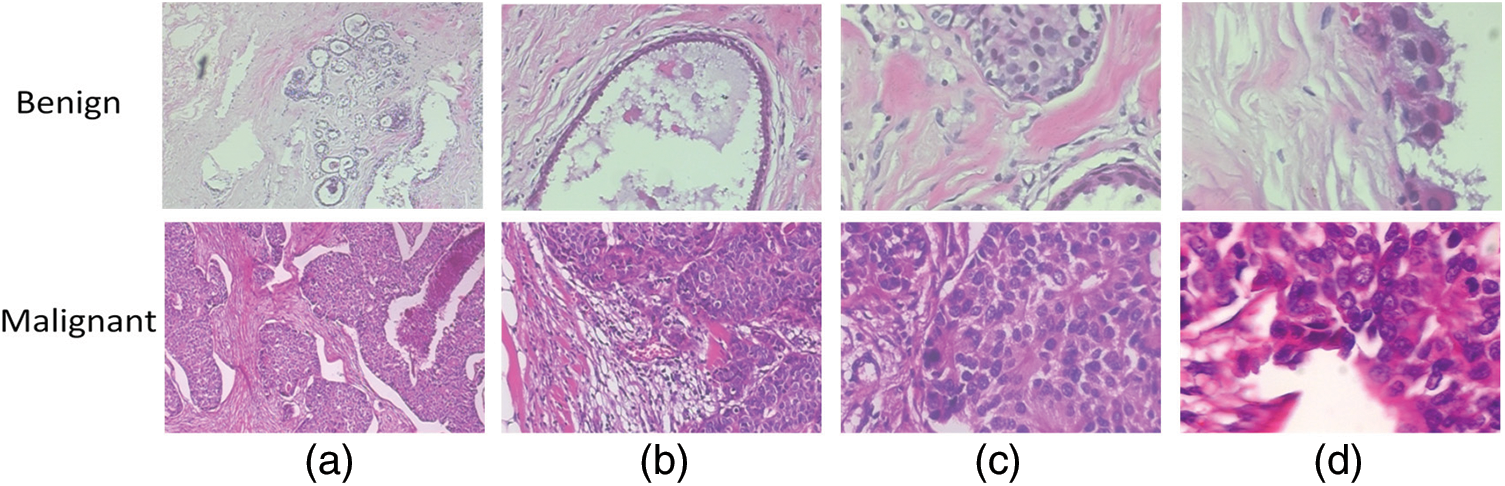
Figure 2: A breast cancer slide at four different magnifications: (a) 40X, (b) 100X, (c) 200X, and (d) 400X

The data needed to be rebalanced, and many different approaches were studied. Under-sampling would include decreasing normal slides to equal the number of cancer slides, but this would diminish the already limited amount of data from the majority class and, as a result, may eliminate beneficial features. If the minority class was oversampled using a method such as the synthetic minority over-sampling technique (SMOTE) [30], the output classes would be more balanced, and the model would have access to more useful information. However, this method is more computationally expensive than the technique currently used, class weights, a simpler technique. Class weighting gives more weight to the class under-represented in the training data when computing the loss function. Class weighting does not involve further manipulation of the training data, given its capacity to meaningfully extend the size of the training data set currently limited in BreakHis 1.0. Fig. 3 shows the results of resampling using SMOTE.

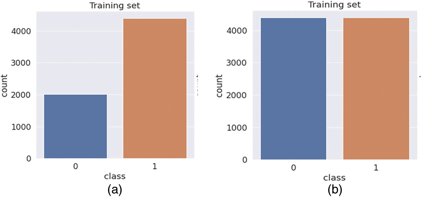
Figure 3: Bar chart showing the output class distribution between the benign and malignant classes within the training data. (a) Before Balancing (b) After Balancing

All datasets used for this inquiry were partitioned into K-fold cross-validation parts with their corresponding ratios. When using XGBOOST, training images are used to build a model, while testing images are utilized to evaluate the model and obtain information from the one that has been trained.

3.2 Preprocessing

Digital image processing yields subtly diverse outcomes when applied to images in various color modes. Converting an image from Red, Green, Blue (RGB) to Luminance, Chrominance (YCBCR) offers many benefits. For image and video compression, transmission, and processing, YCBCR is a color space that separates luminance (brightness) and chrominance (color). Converting an image from RGB to YCBCR reduces color redundancy, which improves image compression. In YCBCR, the luminance channel has the most visual information. Reducing chrominance resolution reduces file size without affecting image quality. YCBCR also handles human-device color perception discrepancies. Electronic gadgets see red, blue, and green equally, but humans see green more. YCBCR handles these variances by segregating luminance and chrominance information. So, the RGB image is converted to YCBCR using the OpenCV library in Python to separate all three components of YCBCR.

3.3 Feature Extraction

Signal processing, data compression, and image analysis are just a few of the many applications of the wavelet transform, a mathematical technique. It takes a signal and breaks it down into a family of wavelets, each of which is a scaled and translated version of the mother wavelet. The wavelet transform can be applied to signals in either continuous or discrete time. Discrete wavelet transforms (DWT) are frequently used for feature extraction and compression in image processing. The DWT breaks down an image into coefficients representing various degrees of detail and approximation. The image is convolved with a collection of filters known as the wavelet filters to extract these coefficients. The DWT can be expressed mathematically as follows:

Wj,k=∑n=0n−1⁡xnφj,k,n(1)

Vj+1,k=Wj,k=∑n=0n−1⁡xn∅j,k,n(2)

where φj,k,n and ∅j,k,n are wavelet and scaling functions, and xn is the original signal. At level j and index k, the wavelet and scaling coefficients are denoted by Wj,k and Vj+1,k.

Image analysis software widely uses texture features and the grey-level co-occurrences matrix (GLCM). Important details are laid out, and useful statistical interface formulas are also laid out [31]. The image’s pixel intensities are ranked by counting how many of each kind there are. An image set’s mean is calculated by:

M=(1m×n)∑0=xm1⁡∑0=yn1⁡f(x.y)(3)

The standard deviation may measure in-homogeneousness because it depicts the probability distribution of the observed population [32]. Standard deviations with larger values publicly reflect the high resolution of the boundaries of an image and are indicative of images with higher intensity levels. Using the described formula, it determined:

S.D(σ)=(1m×n)∑0=xm1⁡∑0=yn1⁡(f(x.y)−M)2(4)

A metric known as “skewness” [32] has been used to quantify the presence or absence of symmetry. Skewness, denoted by Sk(x), is defined as follows for the X probability distribution.

Sk(x)={1m×n}∑{F(x,y)−m}S.D3(5)

The term kurtosis [33] is used to characterize the curvature of the probability distributions of random variables. Kurt of variable x, also known as the kurtosis of a random variable, is defined as:

Kurt(x)={.1m×n}∑(F(x,y)−m)S.D4(6)

A metric known as energy has been applied to the study of visual similarities. The energy variable quantifies how many times the pixelated image may be replicated. The Horalicks’ definition of feature energy in the GLCMs. The second angular moment is another name for it, and its full name is as follows:

En=∑0=xm1⁡∑0=yn1⁡F2(x.y)(7)

By contrast, also known as the resolution of a pixel concerning its neighbors, it is a measurement used to assess the quality of an image.

Con=∑0=xm1⁡∑0=yn1⁡(x(y)2f(x.y))(8)

3.4 Classification

We rely on earlier studies to guide our classification method because feature extraction is more important to our work than building a superior classifier. Our research confirmed the widespread implementation of nonlinear XGBOOST for image classification and the successful attainment of high-quality detection outcomes. For this reason, XGBOOST is our top pick. The DART amplifier is being used. Training and testing are two of several steps in the categorization process. Fig. 1 illustrates a functional breakdown of the system’s workflow. During its formation, the classifier draws heavily on the texture features of the image databases. After wavelet-based feature extraction, we train a classification model with XGBOOST. Every image in the experimental datasets had features extracted for training data. The 10-fold cross-validation technique is employed for this purpose. In order to analyze the data, it was split up into k-segments. On every experimental dataset, the proposed model excels.

3.5 Experimental Setup

Python evaluated texture attributes, and XGBOOST classified counterfeit photos. Several machine-learning methods and extraction parameters were evaluated to enhance accuracy. XGBOOST classified images, and Python 3.11 preprocessed and extracted features. OpenCV and NumPy are popular image-reading and preprocessing libraries. Robotics, autonomous cars, and computer vision use these picture libraries. PyFeat extracts picture features using texture, shape, and color. These traits help machine learning systems classify and recognize items. XGBOOST and Scikit-learn offer decision trees, random forests, and support vector machines. SMOTE is used in machine learning to correct the class imbalance. SMOTE generates artificial minority class samples to balance the dataset and improve classification model accuracy. These Python packages process, extract, classify, and visualize pictures. Matplotlib and Seaborn ease picture analysis and categorization. The DART booster’s default settings use all training samples with a learning rate of 0.1, a maximum tree depth of 6, a subsample ratio of 1, a regularization term of 1, a gamma value of 0.0 (no minimum loss reduction required for splitting), a minimum child weight of 1, and no dropout. K-Fold cross-validation evaluates categorization models. XGBOOST’s cross-validated k-fold datasets were calculated using each fold’s testing set. A Jupyter Notebook with a seventh-generation Dell I7 CPU, 16 GB of RAM, and 1 TB of storage ran all tests.

3.6 Evaluation Measures

Many distinct measures, such as testing accuracy, precision, recall, F1-score, and AUC, are used to evaluate the classification process. When considering the proposed method, the assessment parameter utilized most of the time is accurate. So, in this study, the proposed approach is quantitatively evaluated using the following three parameters:

Accuracy=TP+TNTP+TN+FP+FN(9)

where Accuracy is the total number of correct guesses divided by the total number of correct forecasts, then multiplied by 100 to get a percentage, the percentage of correctly identified samples in the true positive rate is determined using.

Precision=TPTP+FP(10)

Recall=FPTP+FN(11)

In this model, true positive (TP) represents the number of diseases that were correctly recognized, false positive (FP) represents the number of conditions that were misclassified, and false negative represents the number of diseases that should have been discovered but were not (FN). The F1 score is a popular measure for accuracy and recall.

F1score=2×Precision×Recall(Precision+Recall)(12)

Cross-validation (CV) is a resampling methodology utilized to assess machine learning models in a constricted dataset while safeguarding the prediction models against overfitting. On the other hand, K-Fold CV embodies a technique where the given dataset is spliced into K segments or folds, where each fold serves as a testing set at some point. Consider the case of 10-fold cross-validation (K = 10), where the dataset is separated into ten folds, with the first fold testing the model in the first iteration and the remaining folds trained on the model. In the second iteration, the second fold serves as the testing set, whereas the rest function as the training set. This cyclic process repeats until each ten-fold is utilized as the testing set.

4  Results and Analysis

The results of a large-scale experiment to test the proposed method for categorizing breast cancer are presented here. We used the evaluation method mentioned in Section 3.6 to train and score the models. Data was compiled from a wide range of performance assessment tools. The tests were conducted in the following areas:

These areas were the focus of the experiments:

1.    The effectiveness of the proposed framework is measured by XGBOOST for two-class classification across different magnification datasets individually available in BreakHis 1.0.

2.    For two-class classification on the combined dataset, XGBOOST is used to evaluate the efficacy of the suggested framework. Cross-validation uses different assessment metrics to rate the proposed framework on the combined dataset for benign and malignant.

3.    Analysis of how the proposed method stacks up against other, more advanced approaches.

4.1 Evaluation of Proposed Method on 40X, 100X, 200X, and 400X Images from BreakHis 1.0

Table 2 summarizes ten rounds of cross-validation testing of a breast cancer classification model on a 40X magnified dataset. Wavelet transformation and textural features of histopathological images distinguish benign from malignant instances. The table below shows each fold’s benign and malignant classification percentage. The AUC statistic and the number of images utilized in each iteration are shown. All folds have good accuracy ratings of 96.35–99.27 percent. The model correctly classifies benign and malignant cases with good precision, recall, and F1 score values. Wavelet transformation and textural aspects of histopathology images may improve breast cancer classification accuracy and patient outcomes.

When evaluating machine learning models, cross-validation is frequently used. The dataset is partitioned into k folds, and the model is trained k times, with each fold serving as either the validation or training set. The model can be put to the test on new data through cross-validation. Model performance across each cross-validation fold is displayed in fold-wise confusion matrices. For each category, they show the proportion of correct classifications, incorrect classifications, and false negatives. Overfitting, class imbalance, and patterns in model performance can all be identified with this information. Based on the fold-wise confusion matrices presented in Fig. 4, the model achieves high-performance levels for both benign and malignant classes. Depending on the fold, performance may change due to differences in the number of images used per class. Blue boxes in the confusion matrix show samples that are correctly classified.

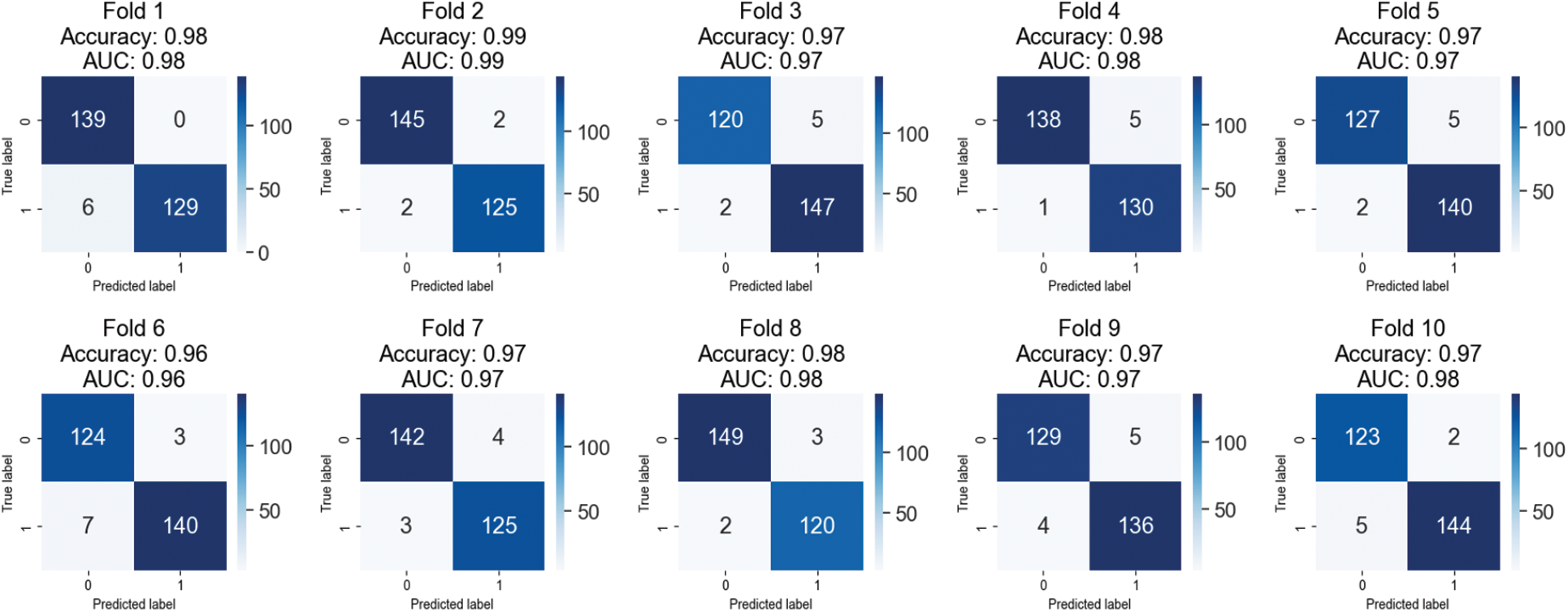
Figure 4: Confusion matrices of testing results on 40X magnified images of BreakHis 1.0

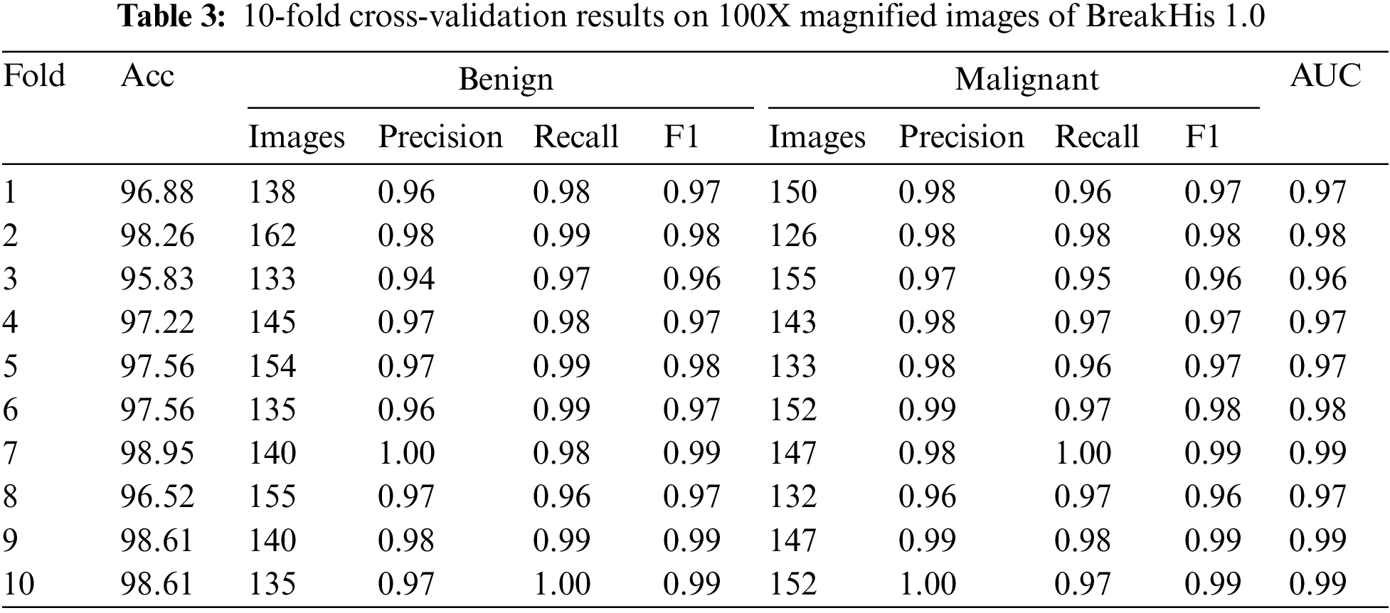
Table 3 displays the outcomes of a 10-fold cross-validation on the BreakHis 1.0 dataset using the proposed approach and a 100X magnification. The table separately lists the accuracy, precision, recall, and F1 score for each fold and benign and cancerous images. We also provide area under the curve (AUC) values for each fold, quantifying the model’s ability to differentiate between benign and cancerous images. The outcomes show that the automated approach is effective and accurate in spotting breast cancer. The high accuracy ratings (95.83–98.95%) demonstrate that the system can successfully categorize various images. The excellent precision, recall, and F1 score scores show how well the system can distinguish between benign and cancerous images. The AUC values demonstrate that the algorithm can distinguish between normal and cancerous images. These findings provide promising evidence for the potential utility of the automated approach in detecting invasive breast cancer.

The confusion matrices shown in Fig. 5 can be used to perform a fold-wise evaluation of a classification model. The model was trained and validated using many folds or data sets. The confusion matrices show how well the model does on each fold. The model’s accuracy and AUC (Area under the Curve) on that fold constitutes its total performance. True positives (TP), true negatives (TN), false positives (FP), and false negatives (FN) are added up for each fold and displayed in the confusion matrix. Metrics such as precision, recall, and F1score can be computed from this data to shed light on the model’s efficacy. The model has performed well with few false positives and negatives, and the accuracy and AUC values are sufficient for most folds. The model’s advantages and disadvantages need more investigation in any case.

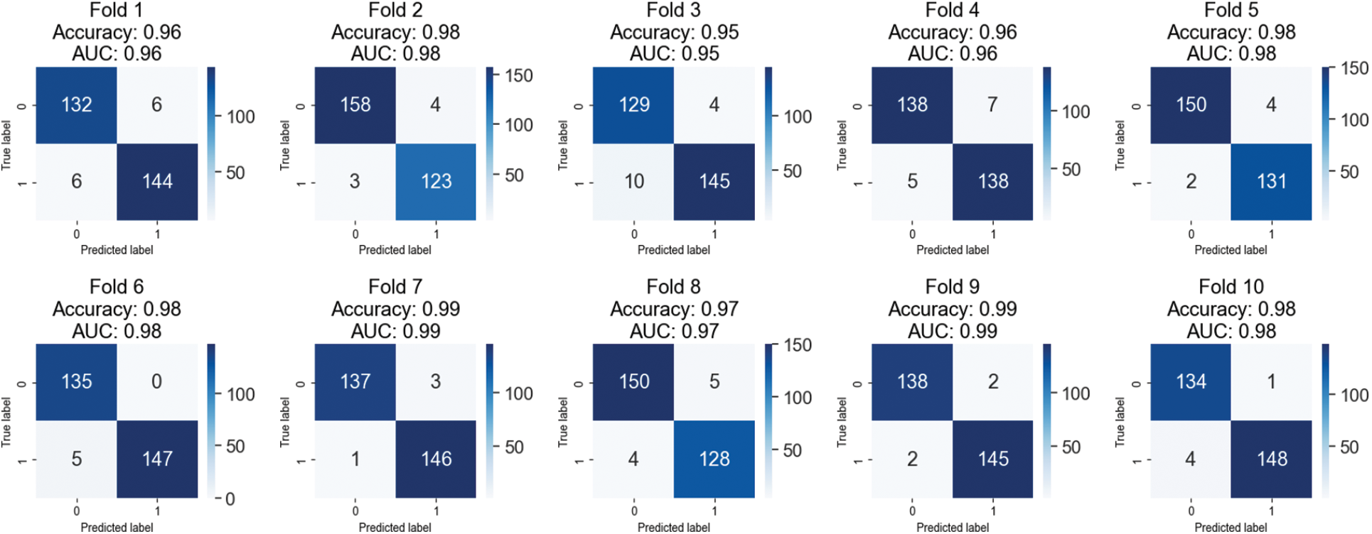
Figure 5: Confusion matrices of testing results on 100X magnified images of BreakHis 1.0

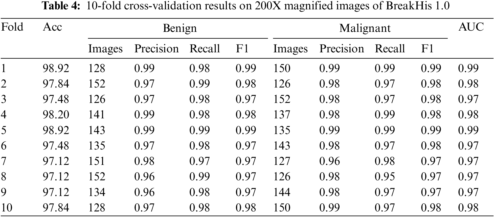
Table 4 displays the outcomes of a 10-fold cross-validation study conducted on images from the BreakHis 1.0 dataset that were magnified by a factor of 200. The cross-validation is represented by “folds,” or rows. Values for accuracy, precision, recall, F1 score, and area under the curve (AUC) are displayed in separate columns for benign and malignant images. Between 97.12% and 98.92%, the fold-wise accuracy is quite high. Both benign and cancerous images have precision values between 0.96 and 0.99. Both healthy and cancerous images have recall values between 0.97 and 0.99. The F1 score values are between 0.97 and 0.99 for healthy and cancerous images. The AUCs are between 0.97 and 0.99. The results show that the model is highly accurate and performs well when identifying benign and malignant breast histopathology images.

Ten iterations of cross-validation were run on a 200-fold-enhanced version of the BreakHis 1.0 dataset, and the findings are displayed in confusion matrices in Fig. 6. Each fold’s accuracy, AUC, and confusion matrix are shown independently. Members of a confusion matrix that fall on the diagonal reflect correctly diagnosed events (benign and malignant), whereas those that fall off the diagonal represent misclassified cases. The model has an adequate area under the curve (AUC). There is some variation in the number of misclassified samples between the different folds. Each additional fold results in a higher rate of false positives (three cases of benign disease misdiagnosed as malignant) and false negatives (five cases of malignant disease misdiagnosed as benign). Areas under the curve that are large are indicative of successful data classification. If there is a big discrepancy between the number of benign and malignant events in this dataset, the class imbalance may be troublesome even if AUC remains unchanged.

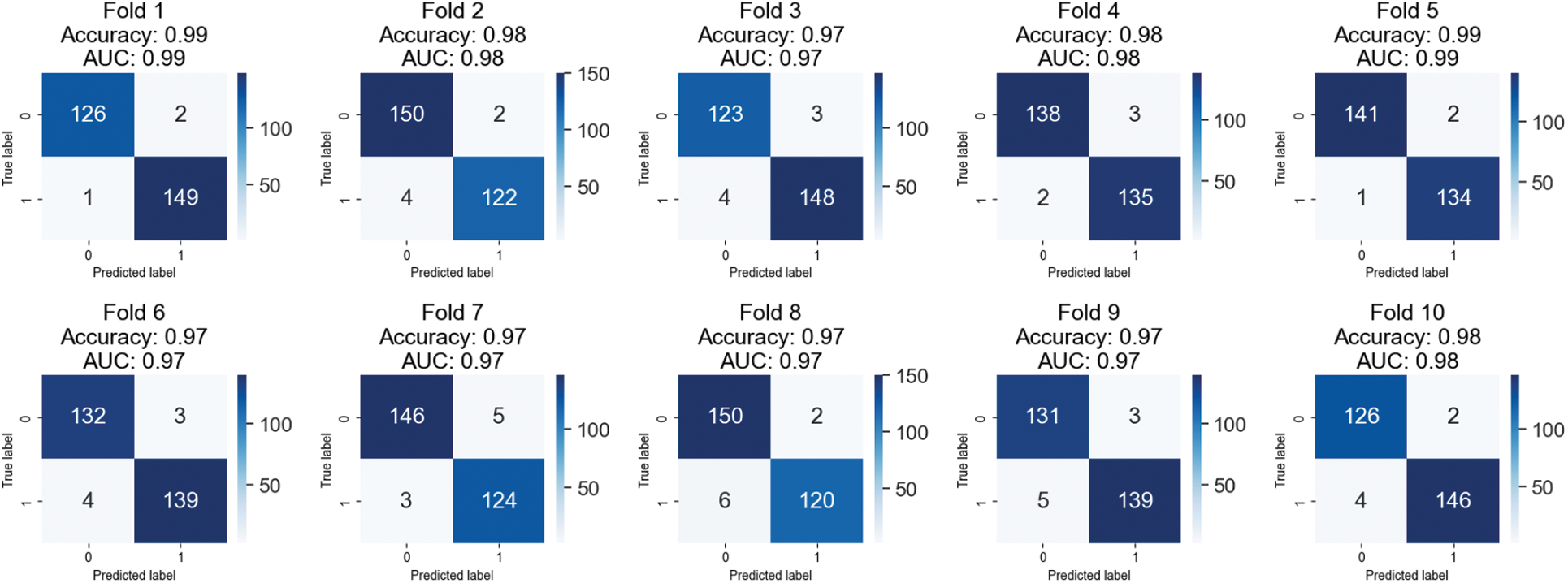
Figure 6: Confusion matrices of testing results on 200X magnified images of BreakHis 1.0

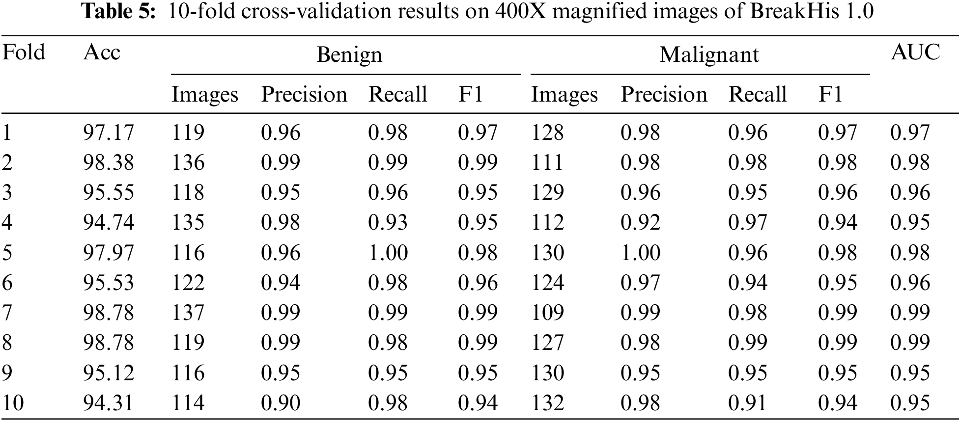
This research used XBOOST to correctly label benign and malignant breast cancer images in a dataset comprising both types of cancer. Table 5 displays the outcomes of a 10-fold cross-validation test conducted on 400X zooms of the BreakHis 1.0 dataset. The table shows each fold’s accuracy, precision, recall, F1 score, and AUC. The table shows that for most folds, the proposed method achieved good accuracy (between 94.31% and 98.78%). High precision and recall values show that the method accurately separates benign from malignant samples. The high area AUC scores, ranging from 0.94 to 0.99, further prove that the proposed technique is a success. Table 5 shows that the proposed approach is a potentially useful strategy for classifying breast cancer images, which can be implemented in clinical settings for early detection and diagnosis.

Fold-wise confusion matrices for the provided classification model are displayed in Fig. 7. The accuracy and AUC (area under the curve) values are presented for each fold, representing the model’s performance on a different portion of the data. Each confusion matrix is a 2 × 2 table, with the first row showing the number of false positives and the second showing the number of false negatives. Correctly classified samples are denoted by items on the diagonal (top left and bottom right), while misclassified samples are denoted by elements off the diagonal (top right and bottom left). The provided data suggests that the model performs better, with accuracy scores between 0.94 and 0.99 and AUC scores between 0.95 and 0.99 throughout the ten folds. It is worth noting that results may differ based on the dataset used. Therefore, additional investigation into the model’s efficacy may be necessary.

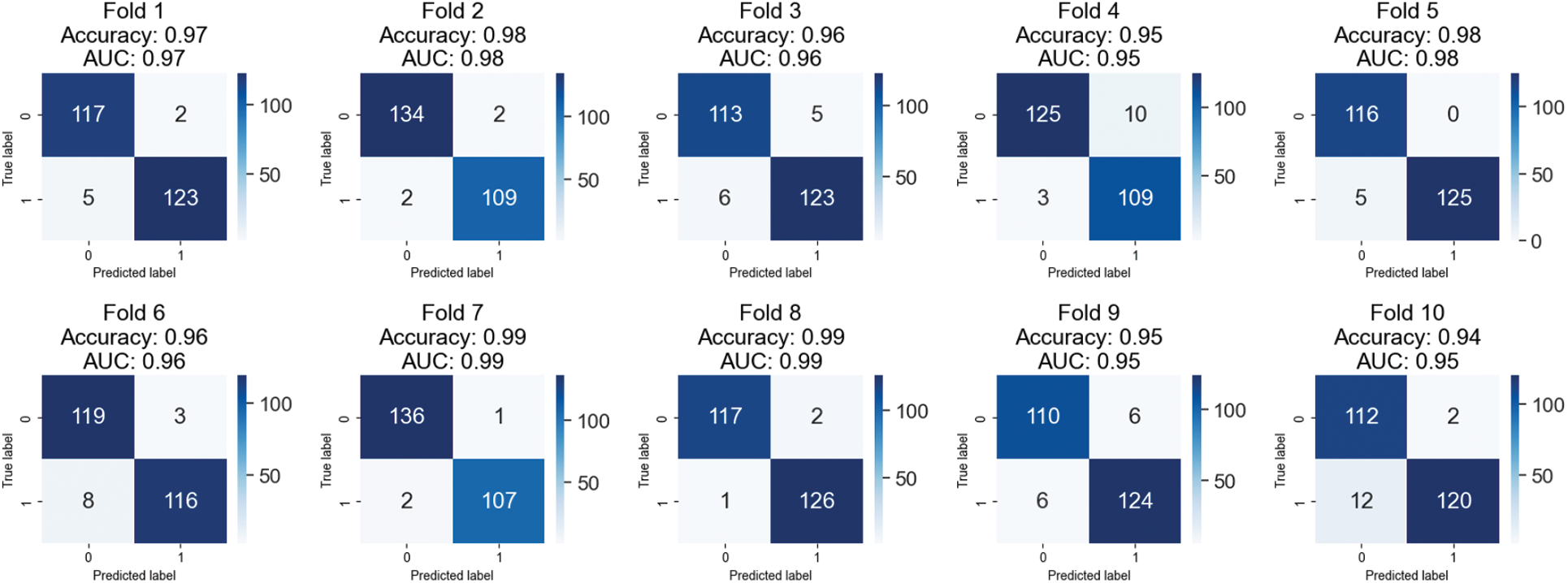
Figure 7: Confusion matrices of testing results on 400X magnified images of BreakHis 1.0

Tables 2 and 3, and Fig. 4 show that the proposed method can successfully identify breast cancer in histological images. Wavelet transformation and textured features of histopathology pictures were used in the suggested study to distinguish between benign and malignant breast cancer. High accuracy, precision, recall, and F1 score results in cross-validation tests show that the models can correctly label a sizable fraction of images. The AUC values also demonstrate that the models can distinguish between normal and cancerous visuals. These results provide preliminary support for the automated invasive breast cancer detection technique, implying that it may improve patient outcomes.

4.2 Performance Evaluation of Proposed Method on Combined Dataset

Table 6 summarizes the results of the BreakHis 1.0 dataset’s application of the XGBOOST algorithm to classify breast cancer patients. Ten-fold cross-validation results show that the model is quite accurate, with a mean of 97.84%. The model’s recall, F1, and accuracy were used to evaluate how well it distinguished between benign and malignant tumors. The F1 score, precision, and recall all stayed in the 0.96 to 0.99 range for the harmless category. The malignant class’s F1 score, recall, and precision were all between 0.97 and 0.99. These results show that the model can distinguish between benign and malignant tumors in breast cancer images. The area under the curve (AUC) was also used to evaluate the model’s performance in identifying benign from malignant tumors. The model has excellent discriminatory power with an AUC in the range of 0.97 and 0.99. The results indicate that the proposed method is a practical strategy for breast cancer categorization based on histological images.

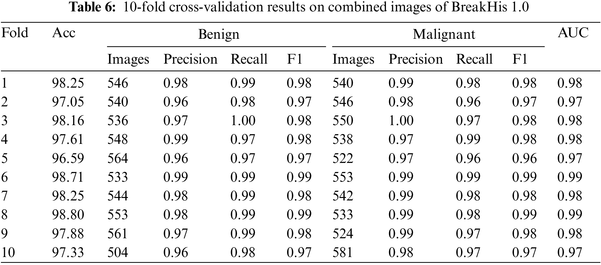
Fig. 8 displays the 10-fold cross-validation results for a breast cancer XGBOOST model’s classification accuracy. Several different dataset folds exist for generating independent training and validation datasets. After each cycle, we log the AUC and accuracy. The confusion matrix provides information about the percentages of correct and incorrect results for each fold. The model has a respectable accuracy of 0.94 to 0.99 across ten folds.

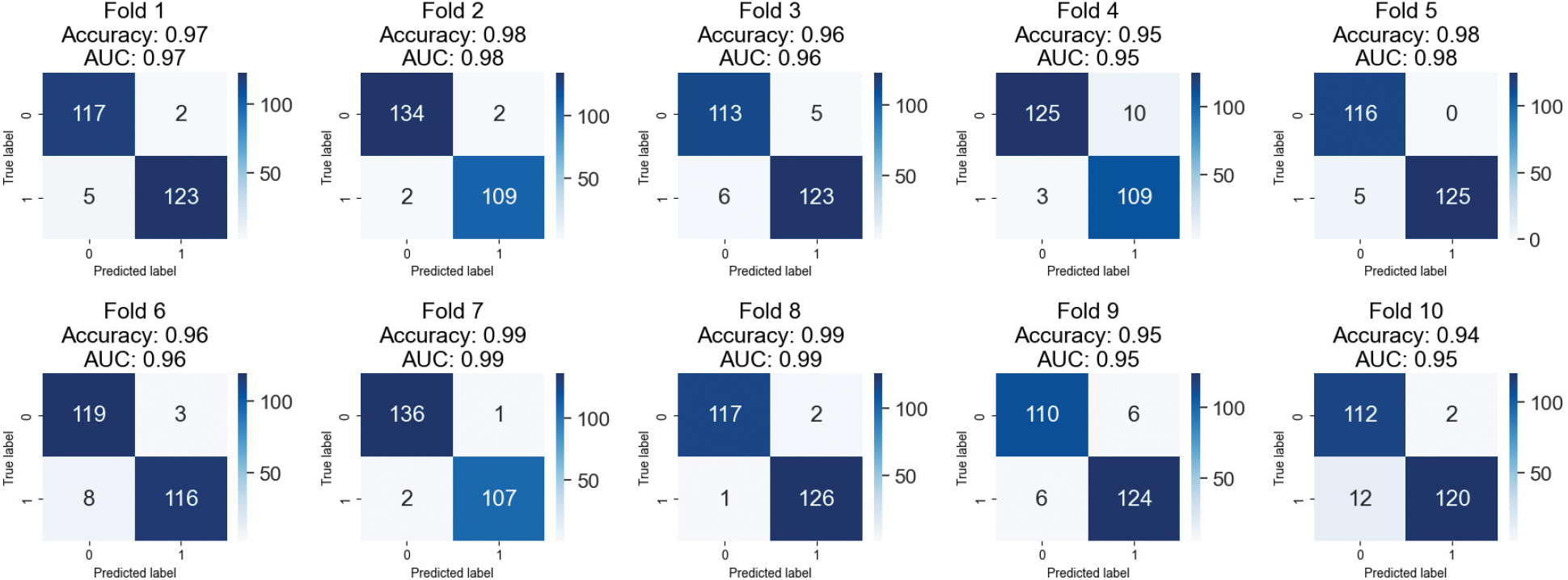
Figure 8: Confusion matrices of testing results on combined images of BreakHis 1.0

Furthermore, the AUC values are rather satisfactory, between 0.95 and 0.99. These findings indicate that the model may be able to distinguish between benign and aggressive breast tumors. The confusion matrices demonstrate that the model correctly classifies occurrences as good or bad. False positives and false negatives are possible, although only very rarely. When a model wrongly detects a benign instance as malignant, this is known as a false positive (FP), and when a model incorrectly identifies a malignant instance as benign, this is known as a false negative (FN). Clinical situations are inherently high-risk, making accounting for this type of error imperative. The proposed method appears to apply to classifying breast cancer. However, more research on larger datasets is required to verify their clinical feasibility.

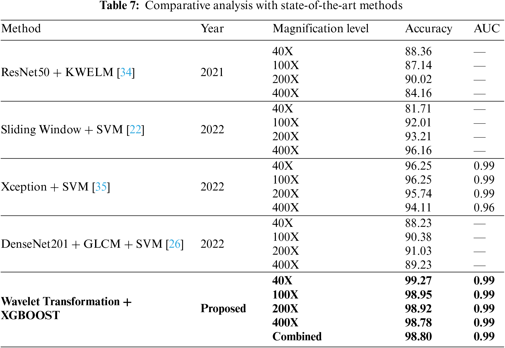
4.3 Comparative Analysis with State-of-Art Methods

Section 2 covers the many methods used to diagnose breast cancer. A few of them use machine learning and deep learning. Different models can be compared using the same data to see how well they perform. Our research included comparing our approach with others that produce comparable results. We compare the suggested method’s accuracy to that of state-of-the-art methods. Table 7 compares the accuracy of various techniques for detecting breast cancer at varying magnification levels. The proposed method is just one of many that can be used; other options are Sliding Window + SVM [13], ResNet50 + KWELM [28], Xception + SVM [29], and DenseNet201 + GLCM + SVM [17]. All measurements, including accuracy and area under the curve, suggest that the proposed strategy is superior. At 40X magnification, the proposed method obtains an accuracy of 99.27%, while at 100X magnification, it achieves an accuracy of 98.95%. Both at 200X and 400X, it gets a 98.92% accuracy rate. Xception plus SVM consistently beats other methods, regardless of zoom level. ResNet50 + KWELM performs moderately better from 40X to 100X but much worse from 100X to 400X. The proposed method shows potential as a robust instrument for detecting breast cancer due to its higher performance.

5  Conclusion

Recognizing malignant images is a vital study topic in the medical field. The purpose of this research is to employ wavelet transformation and texture features in the diagnosis of breast cancer. Our method eliminates the YCBCR channels from an image before extracting blocks of color data. The proposed method is resilient against transformations (rotation, scaling, and distortion) applied to the tumor region. However, we trained and tested our proposed technique on a larger collection of images to increase its efficacy. The classification was performed using the XGBOOST classifier, and feature extraction parameters were optimized for optimum accuracy. Maximum accuracy of 99.27% was reached on the 40X dataset, 98.95% on the 100X dataset, 98.92% on the 200X dataset, 98.78% on the 400X dataset, and 98.80% on the combined dataset using the suggested method. Our findings show that wavelet modification can be used successfully for cancer image recognition. There are, however, some restrictions that must be overcome. For instance, our dataset does not reflect the world as it is because of the biases introduced by Smote. In addition, our approach might need help with more advanced forms of image editing, such as sophisticated geometric transformations or semantic changes at a higher level. In conclusion, our research has aided in advancing wavelet-based methods for recognizing cancer images in medical imagery. To make our method more accurate and stable, we intend to continue investigating this topic by increasing the size of our dataset and investigating additional classification models. The goal is to create a system that can accurately and efficiently categorize multi-class cancer images in real-world settings.

Acknowledgement: None.

Funding Statement: This work was funded by Princess Nourah bint Abdulrahman University Researchers Supporting Project Number (PNURSP2023R236), Princess Nourah bint Abdulrahman University, Riyadh, Saudi Arabia.

Author Contributions: The authors confirm contribution to the paper as follows: study conception and design: A. Akram, M. Hamid, J. Rashid; data collection: A. Akram, F. Hajjej, N. Sarwar; analysis and interpretation of results: A. Arshad, J. Rashid, M. Hamid; draft manuscript preparation: A. Akram, J. Rashid, F. Hajjej, N. Sarwar, M. Hamid. All authors reviewed the results and approved the final version of the manuscript.

Availability of Data and Materials: Data will be provided on request. It is also publicly available.

Conflicts of Interest: The authors declare that they have no conflicts of interest to report regarding the present study.

References

1. C. Mattiuzzi and G. Lippi, “Cancer statistics: A comparison between World Health Organization (WHO) and global burden of disease (GBD),” European Journal of Public Health, vol. 30, no. 5, pp. 1026–1027, 2020. [Google Scholar] [PubMed]

2. P. Xie, K. Zuo, J. Liu, M. Chen, S. Zhao et al., “Interpretable diagnosis for whole-slide melanoma histology images using convolutional neural network,” Journal of Healthcare Engineering, vol. 2021, pp. 8396438, 2021. https://doi.org/10.1155/2021/8396438 [Google Scholar] [PubMed] [CrossRef]

3. A. Cruz-Roa, H. Gilmore, A. Basavanhally, M. Feldman, S. Ganesan et al., “Accurate and reproducible invasive breast cancer detection in whole-slide images: A deep learning approach for quantifying tumor extent,” Scientific Reports, vol. 7, no. 1, pp. 1–14, 2017. [Google Scholar]

4. J. Rashid, I. Khan, G. Ali, S. U. Rehman and F. Alturise, “Real-time multiple guava leaf disease detection from a single leaf using hybrid deep learning technique,” Computers, Materials & Continua, vol. 74, no. 1, pp. 1235–1257, 2023. [Google Scholar]

5. H. Chu, M. R. Saeed, J. Rashid, M. T. Mehmood, I. Ahmad et al., “Deep learning method to detect the road cracks and potholes for smart cities,” Computers, Materials & Continua, vol. 75, no. 1, pp. 1863–1881, 2023. [Google Scholar]

6. A. Akram, D. A. Jaffar, D. W. Iqbal, M. S. Ali, M. U. Tariq et al., “A robust and scale invariant method for image forgery classification using edge weighted local texture features,” Jilin Daxue Xuebao (Gongxueban)/Journal of Jilin University (Engineering and Technology Edition), vol. 41, no. 12, pp. 330–344, 2022. [Google Scholar]

7. A. Akram, S. Ramzan, A. Rasool, A. Jaffar, U. Furqan et al., “Image splicing detection using discriminative robust local binary pattern and support vector machine,” World Journal of Engineering, vol. 19, pp. 459–466, 2022. [Google Scholar]

8. X. Wang, Y. Peng, L. Lu, Z. Lu, M. Bagheri et al., “ChestX-ray8: Hospital-scale chest X-ray database and benchmarks on weakly-supervised classification and localization of common thorax diseases,” in Proc. of IEEE Conf. on Computer Vision and Pattern Recognition, Honolulu, HI, USA, Computer Vision Foundation, pp. 2097–2106, 2017. [Google Scholar]

9. D. C. Cireşan, A. Giusti, L. M. Gambardella and J. Schmidhuber, “Mitosis detection in breast cancer histology images with deep neural networks,” in Medical Image Computing and Computer-Assisted Intervention–MICCAI 2013, Nagoya, Japan, Springer, vol. 16, pp. 411–418, 2013. [Google Scholar]

10. Z. Hameed, S. Zahia, B. Garcia-Zapirain, J. Javier Aguirre and A. Maria Vanegas, “Breast cancer histopathology image classification using an ensemble of deep learning models,” Sensors, vol. 20, no. 16, pp. 43–73, 2020. [Google Scholar]

11. A. Rakhlin, A. Shvets, V. Iglovikov and A. A. Kalinin, “Deep convolutional neural networks for breast cancer histology image analysis,” in Proc. of Image Analysis and Recognition: 15th Int. Conf. ICIAR 2018, Varzim, Portugal, Springer, vol. 15, pp. 737–744, 2018. [Google Scholar]

12. V. S. Parekh and M. A. Jacobs, “Deep learning and radiomics in precision medicine,” Expert Review of Precision Medicine And Drug Development, vol. 4, no. 2, pp. 59–72, 2019. [Google Scholar] [PubMed]

13. K. Sirinukunwattana, S. E. A. Raza, Y. W. Tsang, D. R. Snead, I. A. Cree et al., “Locality sensitive deep learning for detection and classification of nuclei in routine colon cancer histology images,” IEEE Transactions on Medical Imaging, vol. 35, no. 5, pp. 1196–1206, 2016. [Google Scholar] [PubMed]

14. S. Tummala, J. Kim and S. Kadry, “BreaST-Net: Multi-class classification of breast cancer from histopathological images using ensemble of swin transformers,” Mathematics, vol. 10, no. 21, pp. 4109, 2022. [Google Scholar]

15. O. Stephen and M. Sain, “Using deep learning with bayesian-gaussian inspired convolutional neural architectural search for cancer recognition and classification from histopathological image frames,” Journal of Healthcare Engineering, vol. 2023, pp. 1–9, 2023. [Google Scholar]

16. V. C. S. Rao, P. Radhika, N. Polala and S. Kiran, “Logistic regression versus XGBoost: Machine learning for counterfeit news detection,” in 2021 Second Int. Conf. on Smart Technologies in Computing, Electrical and Electronics (ICSTCEE), Bengaluru, India, pp. 1–6, 2021. [Google Scholar]

17. J. Zhang, X. Wei, C. Che, Q. Zhang and X. Wei, “Breast cancer histopathological image classification based on convolutional neural networks,” Journal of Medical Imaging and Health Informatics, vol. 9, no. 4, pp. 735–743, 2019. [Google Scholar]

18. S. C. Wetstein, V. M. T. de Jong, N. Stathonikos, M. Opdam, G. M. H. E. Dackus et al., “Deep learning-based breast cancer grading and survival analysis on whole-slide histopathology images,” Scientific Reports, vol. 12, no. 1, pp. 15102, 2022. [Google Scholar] [PubMed]

19. M. A. Wakili, H. A. Shehu, M. H. Sharif, M. H. U. Sharif, A. Umar et al., “Classification of breast cancer histopathological images using DenseNet and transfer learning,” Computational Intelligence and Neuroscience, vol. 2022, no. 1, pp. 1–31, 2022. [Google Scholar]

20. R. R. Kadhim and M. Y. Kamil, “Evaluation of machine learning models for breast cancer diagnosis via histogram of oriented gradients method and histopathology images,” International Journal on Recent and Innovation Trends in Computing and Communication, vol. 10, no. 4, pp. 36–42, 2022. [Google Scholar]

21. Y. D. Zhang, S. C. Satapathy, D. S. Guttery, J. M. Górriz and S. H. Wang, “Improved breast cancer classification through combining graph convolutional network and convolutional neural network,” Information Processing & Management, vol. 58, no. 2, pp. 102439, 2021. [Google Scholar]

22. A. Alqudah and A. M. Alqudah, “Sliding window based support vector machine system for classification of breast cancer using histopathological microscopic images,” IETE Journal of Research, vol. 68, no. 1, pp. 59–67, 2022. [Google Scholar]

23. D. Clement, E. Agu, M. A. Suleiman, J. Obayemi, S. Adeshina et al., “Multi-class breast cancer histopathological image classification using multi-scale pooled image feature representation (MPIFR) and one-versus-one support vector machines,” Applied Sciences, vol. 13, no. 1, pp. 156–170, 2023. [Google Scholar]

24. H. Seo, L. Brand, L. S. Barco and H. Wang, “Scaling multi-instance support vector machine to breast cancer detection on the BreaKHis dataset,” Bioinformatics, vol. 38, no. 1, pp. i92–i100, 2022. [Google Scholar] [PubMed]

25. R. Saturi and P. Chand Parvataneni, “Histopathology breast cancer detection and classification using optimized superpixel clustering algorithm and support vector machine,” Journal of the Institution of Engineers (IndiaSeries B, vol. 103, no. 5, pp. 1589–1603, 2022. [Google Scholar]

26. Y. Hao, L. Zhang, S. Qiao, Y. Bai, R. Cheng et al., “Breast cancer histopathological images classification based on deep semantic features and gray level co-occurrence matrix,” PLoS One, vol. 17, no. 5, pp. e0267955, 2022. [Google Scholar] [PubMed]

27. M. U. Rehman, S. Akhtar, M. Zakwan and M. H. Mahmood, “Novel architecture with selected feature vector for effective classification of mitotic and non-mitotic cells in breast cancer histology images,” Biomedical Signal Processing and Control, vol. 71, no. 1, pp. 103212, 2022. [Google Scholar]

28. A. A. Joseph, M. Abdullahi, S. B. Junaidu, H. H. Ibrahim and H. Chiroma, “Improved multi-classification of breast cancer histopathological images using handcrafted features and deep neural network (dense layer),” Intelligent Systems with Applications, vol. 14, no. 1, pp. 200066, 2022. [Google Scholar]

29. F. A. Spanhol, L. S. Oliveira, C. Petitjean and L. Heutte, “Breast cancer histopathological image classification using convolutional neural networks,” in Proc. of 2016 Int. Joint Conf. on Neural Networks (IJCNN), Vancouver, BC, Canada, pp. 2560–2567, 2016. [Google Scholar]

30. N. V. Chawla, K. W. Bowyer, L. O. Hall and W. P. Kegelmeyer, “SMOTE: Synthetic minority over-sampling technique,” Journal of Artificial Intelligence Research, vol. 16, pp. 321–357, 2002. [Google Scholar]

31. P. Mohanaiah, P. Sathyanarayana and L. GuruKumar, “Image texture feature extraction using GLCM approach,” International Journal of Scientific and Research Publications, vol. 3, no. 5, pp. 1–5, 2013. [Google Scholar]

32. A. Mustaqeem, A. Javed and T. Fatima, “An efficient brain tumor detection algorithm using watershed & thresholding based segmentation,” International Journal of Image, Graphics and Signal Processing, vol. 4, no. 10, pp. 34, 2012. [Google Scholar]

33. M. Prastawa, E. Bullitt, S. Ho and G. Gerig, “A brain tumor segmentation framework based on outlier detection,” Medical Image Analysis, vol. 8, no. 3, pp. 275–283, 2004. [Google Scholar] [PubMed]

34. S. Saxena, S. Shukla and M. Gyanchandani, “Breast cancer histopathology image classification using kernelized weighted extreme learning machine,” International Journal of Imaging Systems and Technology, vol. 31, no. 1, pp. 168–179, 2021. [Google Scholar]

35. S. Sharma and S. Kumar, “The Xception model: A potential feature extractor in breast cancer histology images classification,” ICT Express, vol. 8, no. 1, pp. 101–108, 2022. [Google Scholar]