Optimization of CNC Turning Machining Parameters Based on Bp-DWMOPSO Algorithm

1  Introduction

With the development of computer technology, optimization algorithms are gradually applied in various fields. Frequently-used data modelling methods mainly include the Response Surface Methodology [1,2], Back Propagation Neural Network (BPNN) [3,4]. Support Vector Regression [5,6] and Gradient Boosted Regression Tree [7]. In order to better solve the optimization problem of CNC turning machining parameters, scholars at home and abroad have conducted a lot of research. Wang et al. proposed a multi-objective optimization method for CNC turning machining parameters based on the Response Surface Methodology and Artificial Bee Colony Algorithm, which has better distribution and convergence of optimization algorithms [8]. Wang et al. established a mathematical model of machining cost and CNC cutting machining efficiency, which was solved by the Hybrid Multi-Objective Particle Swarm Optimization (HMOPSO). They used the Analytical Hierarchy Process for the final decision on the optimal combination of cutting parameters [9]. Meanwhile, Deng et al. explored the applicability of deep reinforcement learning in machining parameter optimization problems and proposed a deep reinforcement learning-based optimization method for CNC Milling Process Parameters [10]. For materials such as aluminium 6063, Osoriopinzon et al. [11] constructed optimization functions using the Response Surface Methodology and Artificial neural networks to solve multi-objective optimization problems such as cutting forces, microstructure refinement and material removal rate, and finally used particle swarm algorithms for optimization solutions. Van [12] used BPNN to construct an optimization model of machining parameters with cutting forces, vibration and energy consumption and realized the multi-objective optimization by multi-objective particle swarm algorithm, which provides an effective solution for the parameter optimization of high-speed milling. Li et al. [13] used the response surface methodology to model the relationship between cutting forces and machining parameters for CNC machining. Based on this, they constructed a multi-objective optimization model which considered cutting force, R-value and surface roughness, and used an improved teaching optimization algorithm to solve the model. He et al. [14] simultaneously considered cutting force, machining time and energy consumption in the carbon steel machining process, established a correlation relation model between each objective and machining parameters through theoretical analysis and empirical formulas. They obtained the Pareto front of the problem by using a decomposition-based multi-objective evolutionary algorithm to find the optimal solution. In order to make the Particle Swarm Optimization (PSO) in the late iteration still have a chance to jump out of the local optimal solution, Wang et al. [15] used methods that can deal with the stopping and receding state particles and random fluctuating inertia weight. Geng et al. [16] designed a PSO algorithm based on an orthogonal experiment mechanism to improve the convergence speed of the algorithm. Wang et al. [17] studied the problem of falling material or unsmooth deep drawing of needle tooth molds in the machining process. They constructed a Bp neural network by using the relationship between the cutting-edge parameters, shear strength and cut-off displacement, and used the experimental results to verify the correctness and reliability of the predicted optimal tooth mold cutting-edge parameters. For the problem of excessive local deformation of the parts in the machining process of the annular thin-walled part, Han et al. [18] proposed an optimization method for milling parameters of annular thin-walled parts with an improved particle swarm algorithm.

In summary, the research direction of optimization of CNC turning machining parameters using optimization algorithms mainly focuses on the algorithm’s global search ability, stability and convergence speed, etc. In related research, there is a lack of research on the machining reliability of the optimized machining parameters, such as whether the optimized parameters can meet the machining accuracy and surface roughness (Ra). Therefore, this paper proposes a Bp Neural Network-Improved Multi-Objective Particle Swarm Algorithm. The difference between it and other algorithms is that the algorithm fully combines the advantages of the Bp neural network’s learning ability, strong generalization ability and particle swarm algorithm’s strong global search ability, which can improve the machining efficiency under the premise of ensuring the machining quality. Consequently, this algorithm is more suitable for the optimization of CNC turning machining parameters.

The research objective of this paper is to establish the relationship model between machining accuracy, surface roughness and machining parameters during the CNC turning machining process by using the powerful approximation ability and learning ability of the Bp neural network. Then, the improved multi-objective particle swarm algorithm is used to optimize the multi-objective function in order to obtain a set of optimal machining parameter combinations. And the obtained parameters can not only meet the requirements of machining accuracy and surface roughness in the machining process but also consider the optimization of other machining performance indicators, thus improving productivity, reducing costs, and ensuring that the quality and performance of machined parts meet the requirements.

The research in this paper has three main points: (1) this paper analyzes the problems of the traditional multi-objective particle swarm algorithm and introduces the Bp neural network algorithm and the Dynamic Weight Multi-Objective Particle Swarm Algorithm; (2) this paper proposes an optimization method of CNC turning machining parameters based on the improved particle algorithm; (3) a case study is used to verify the effectiveness of the method.

2  Algorithm Analysis

2.1 Selection of Optimization Algorithm

Multi-Objective Particle Swarm Optimization (MOPSO) is a heuristic optimization algorithm for solving multi-objective optimization problems. The basic idea of the algorithm is to find the optimal solution set by maintaining a population of particles and iteratively updating them continuously.

However, the algorithm cannot deal with classification and regression problems. When it is applied to solve the CNC turning parameter optimization problem, the resulting machining parameters cannot be directly applied in actual production machining, so it is necessary to judge whether the resulting machining accuracy and surface quality meet the requirements. The Bp neural network (algorithm) has strong adaptability and generalization ability, which is suitable for processing classification and regression problems. Therefore, this paper combines Bp neural network and MOPSO to solve the problem better and introduces the dynamic weighting strategy to improve the performance of the algorithm.

2.2 Bp Neural Network

Bp neural network, also known as Back Propagation Neural Network, is a frequently-used artificial neural network structure for solving classification and regression problems. The network consists of the input, the hidden and the output layers, where the hidden layer can be multiple layers [19]. The structure of a Bp neural network is shown in Fig. 1.

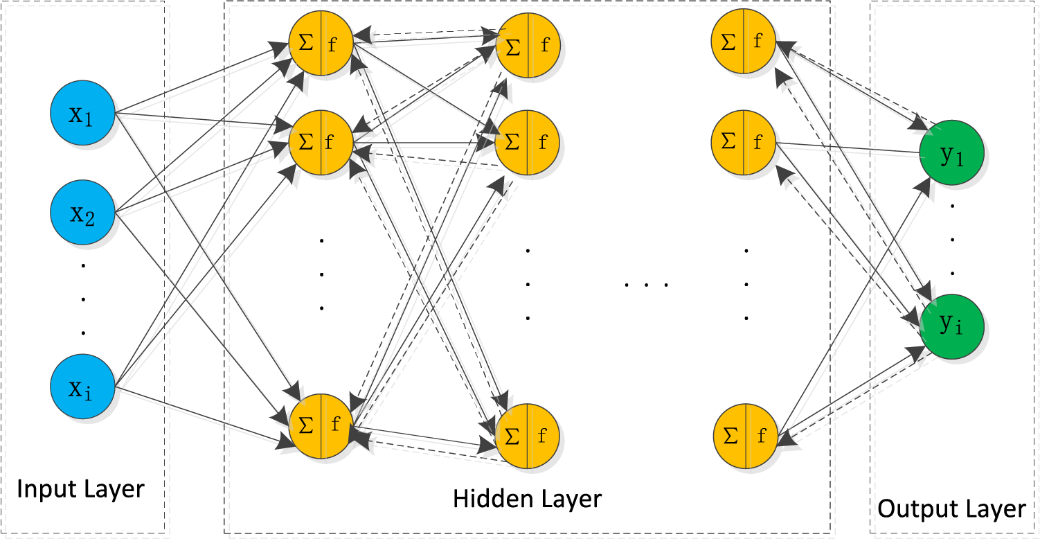
Figure 1: Bp neural network structure chart

The training process of the Bp neural network consists of two steps: forward propagation and backward propagation. In the structure shown in Fig. 1, each layer contains multiple neurons (nodes), and each neuron has an activation function. When the model is working, these neurons are first transmitted forward in the order of the input, hidden and output layers (in the direction of the solid line). After that, the error is transmitted in the reverse direction from the output layer to the hidden layer within the model, that is, the transmission represented by the dashed line in Fig. 1. The function of the transmission is to transmit the error between the actual output and the desired output and to continuously adjust the weights (w) and the bias (b) in the formula in order to achieve the reduction of the error. The specific formulas are as follows:

yi=φ(∑i=1nwji∗xi+bj)(1)

where: yi denotes the output of the jth neuron; xi denotes the ith input feature; wji denotes the connection weight between the ith input feature and the jth neuron; bj denotes the bias of the jth neuron; φ() denotes the activation function.

δj=φ'(netj)*∑kwkj*δk(2)

where: δj denotes the error of the jth neuron; netj denotes the input of the jth neuron; φ′() denotes the derivative of the activation function; wkj denotes the connection weight between the jth neuron and the kth neuron; δk denotes the error of the kth neuron.

Δwji=θ∗δj∗xi(3)

where: Δwji denotes the update of the connection weight between the ith input feature and the jth neuron; θ denotes the learning rate; δj denotes the error of the jth neuron; and xi denotes the value of the ith input feature.

2.3 Dynamic Weighted Multi-Objective Particle Swarm Algorithm

2.3.1 Principle of Dynamic Weighted Multi-Objective Particle Swarm Algorithm

As a swarm intelligence algorithm, the Dynamic Weighted Multi-Objective Particle Swarm Optimization (DWMOPSO) has the advantages of fast convergence and strong optimality search [20]. It searches for the optimal solution based on the Pareto superiority relation. The particle updates itself by tracking two “extremes”: the first extremum, called the individual extremum point, is the best solution found by the particle itself, which is denoted by Pbest, and the other extremum, called the global optimal solution, is the current optimal solution found by the whole population, which is denoted by Gbest. In MOPSO, each particle corresponds to its own Gbest, while the single-objective particle swarm algorithm shares one global extreme point for the whole particle swarm. Meanwhile, DWMOPSO improves the algorithm’s performance by dynamically adjusting the inertia weights. The principle of DWMOPSO is as follows:

1) Initialization: Initialize a particle swarm, including N particles. Each particle has a random position and velocity. The position and velocity is a vector, and the dimension of the vector is equal to the number of independent variables of the function. Each particle should record its current best position Pbest and best fitness pbest_val, as well as the current particle in the current particle in the Pareto optimal set.

2) Update the position and velocity: Each particle updates its velocity and position, according to the following equations:

vi(t+1)=w∗vi(t)+c1∗rand∗(Gbesti−xi(t))+c2∗rand∗(Pbesti−xi(t))(4)

xi(t+1)=xi(t)+vi(t+1)(5)

where: w is the inertia weight; c1 and c2 is the acceleration constant; rand is a random number in the range [0, 1]; Pbesti is the current best position of the particle i; Gbesti is the local optimal solution.

3) Dynamic weighting strategy: The dynamic weight controls the speed of particle movement and the probability of jumping out of the local optimal solution. In DWMOPSO, the inertia weight decreases as the number of iterations increases. As shown in Eq. (6):

w=ws−(ws−we)∗(iterniter)∧2(6)

where: we and ws are the upper and lower bounds of the dynamic weight; iter is the current number of iterations; niter is the maximum number of iterations.

2.3.2 Steps of the Dynamic Weight Multi-Objective Particle Swarm Algorithm

N randomly selected particles constitute a particle swarm, and each particle is a multidimensional vector. The flow chart of the DWMOPSO algorithm is shown in Fig. 2.

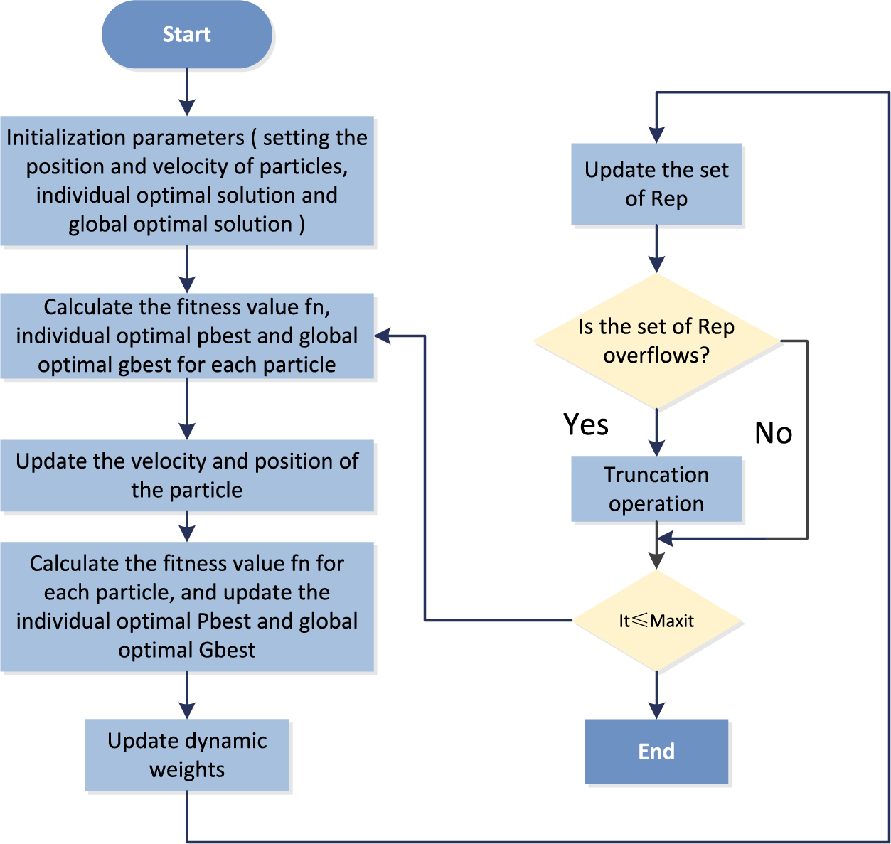
Figure 2: Flow chart of the dynamic weighted multi-objective particle swarm algorithm

Step 1: Initialize the algorithm and set the initialization parameters such as population number, the maximum number of iterations, velocity and displacement of particles, etc.

Step 2: Calculate the fitness value of each particle, and update individual optimal Pbest and global optimal Gbest according to the fitness of the particle.

Step 3: Update the velocity and position of the particle according to the individual optimal solution, global optimal solution, velocity, position and inertia weight of the current particle at the current position.

Step 4: Calculate the fitness value fitness of each particle and update the individual optimal Pbest and the global optimal Gbest.

Step 5: Based on the current iteration number iter, the total iteration number niter, the initial value of inertia weight ws and the final value of inertia weight we, calculate the current inertia weight w.

Step 6: Update the rep set; determine whether the rep set overflows; get the current non-dominated solution.

Step 7: If the number of iterations iter reaches the maximum number of iterations niter, the algorithm ends and outputs the final non-dominated solution set; otherwise, increase the number of iterations iter and return to Step 2.

3  Bp-DWMOPSO Algorithm

3.1 Introduction of Bp-DWMOPSO Algorithm

The Improved Multi-Objective Particle Swarm Algorithm (Bp-DWMOPSO) proposed in this paper is an improved algorithm based on the Bp neural network model and the Dynamic Weight Multi-Objective Particle Swarm Algorithm Model. The algorithm has strong generalization ability and interpretability and can achieve good results when applied to the optimization of CNC turning machining parameters.

3.2 Construction of Bp-DWMOPSO Algorithm

The structure diagram of the Bp-DWMOPSO algorithm is shown in Fig. 3.

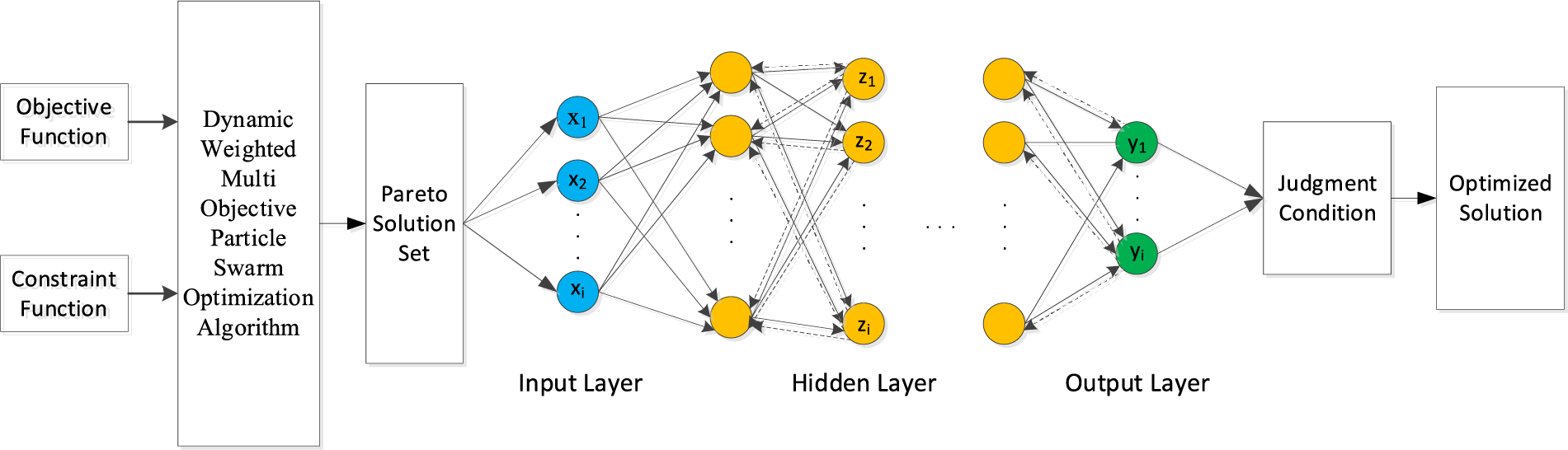
Figure 3: Structure chart of the Bp-DWMOPSO algorithm

As seen in Fig. 3, the Bp-DWMOPSO algorithm solves the problem in the following steps:

Step 1: According to the objective function and constraint function, the dynamic weight multi-objective particle algorithm solves the problem and derives the Pareto solution set.

Step 2: The solutions in the Pareto solution set are substituted into the Bp neural network model to derive the predicted values.

Step 3: After substituting the predicted values into the judgment function for comparison, the solutions that meet the requirements are output; otherwise they are removed.

The solution set screening formula is as follows:

xi=mpi,(i=1,2,…,n)(7)

yi=φ(∑i=1nwji∗xi+bj)(8)

f(y1,y2,…,yi)={1,yi≤y0,others,(i=1,2,…,n)(9)

where: mpi denotes the solution in the Pareto solution set; yi denotes the output of the jth neuron; xi denotes the ith input feature; wji denotes the connection weight between the ith input feature and the jth neuron; bj denotes the bias of the jth neuron; φ(x) denotes the activation function; f(x) denotes the judgment function, and when f(x)=1, output the solution; otherwise remove the solution.

3.2.1 Data Acquisition Methods

The construction of the Bp-DWMOPSO algorithm requires the acquisition of training data. There are various methods of data acquisition, such as orthogonal experiments, single-factor experiments, and multi-factor experiments. According to the characteristics of CNC turning machining parameters, this paper uses equal probability orthogonal experiments to obtain the required data, and this experimental method is a multi-factor multi-level experimental design method. The advantages of this experimental method: (1) It saves experimental cost and time and significantly reduces the number of experiments; (2) It has a balance between the levels of factors, thus reducing the influence of random errors; (3) It can reveal the mutual influence between different factors and discover the main and secondary influencing factors.

3.2.2 Data Preprocessing Methods

Data preprocessing is one of the key steps in optimization model building to ensure that the input data is suitable for the training and learning process of the algorithm. In this paper, the following steps are used to preprocess the data, and the flow of data preprocessing is shown in Fig. 4.

Figure 4: Flow chart of data preprocessing

Step 1: Data Cleaning: Before starting to build the optimization model, the raw data needs to be cleaned. This includes dealing with missing values, abnormal values and noisy data. This paper uses equal probability orthogonal experiments to collect data. This experimental method can effectively avoid the appearance of data such as missing values, abnormal values and noise data, so the collected data do not need to be cleaned and processed.

Step 2: Feature Selection: Feature selection is to choose the most relevant and valuable features from the raw data in order to reduce the data dimension and avoid overfitting. This paper uses the Pearson Correlation Coefficient Method for feature selection. The Pearson Correlation Coefficient expression formula is as follows:

r=1n−1∑i=1n(Xi−X¯σX)(Yi−Y¯σY)(10)

where: X¯ and σX are the standardized score, the sample mean and sample standard deviation for Sample Xi respectively; Y¯ and σY are the standardized score, sister mean and sample standard deviation for Sample Yi, respectively.

Step 3: Data Normalization: In the process of building the optimization model, the range and distribution of the input data may have an impact on the training effect of the model. Therefore, the input data are generally normalized to have similar scales and distributions. This paper uses the maximum-minimum normalization (Min-Max Scaling) method, and the expression is as follows:

Xscale=X−XminXmax−Xmin(11)

where: Xscale is the normalized data; X is the sample data value; Xmin is the sample data minimum; Xmax is the sample data maximum.

Step 4: Data Partition: Divide the data set into the training set, validation set and testing set. And the purpose of dividing the data set is to conduct model training, parameter tuning and performance evaluation.

3.2.3 Characteristic Parameters of the Model

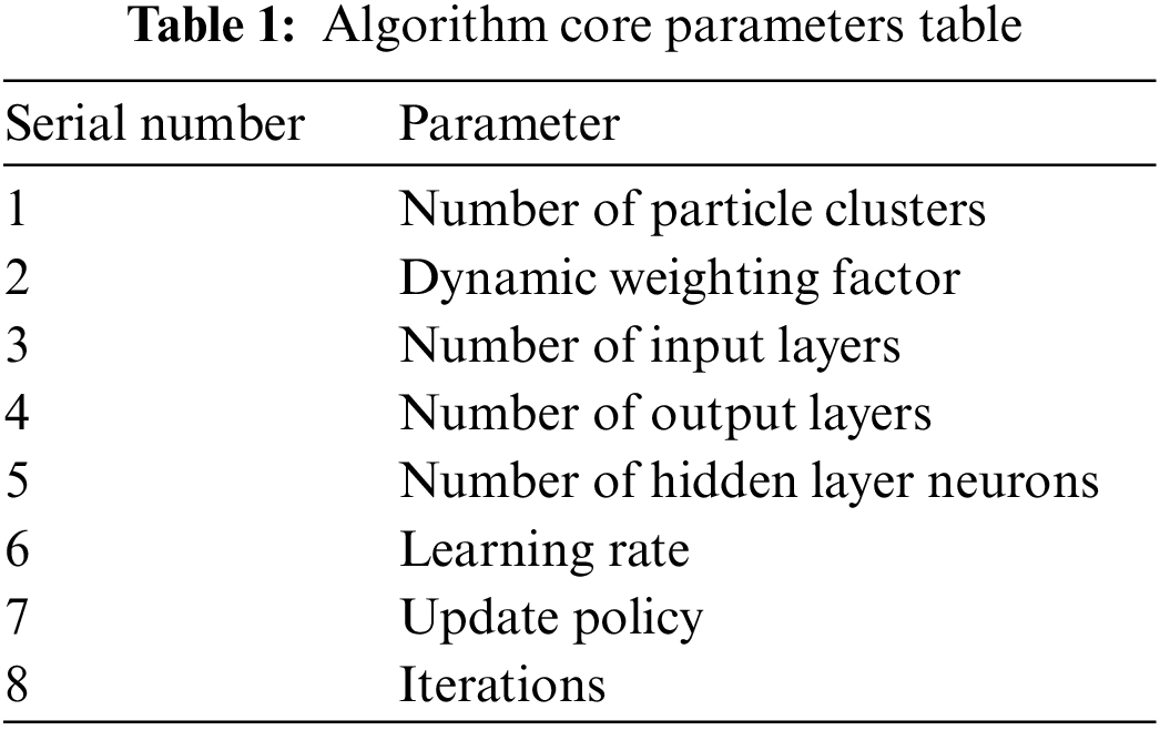
The parameters are one of the core components of the model, and they are critical to the performance and effectiveness of the algorithm. Different parameter values can lead to different algorithm performance. Therefore, the correct selection and adjustment of parameters have an important impact on the performance and effect of the algorithm. For the Bp-DWMOPSO algorithm proposed in this paper, the parameters shown in Table 1 are set as the core parameters of the algorithm to improve the performance of the algorithm, such as accuracy, stability and generalization ability.

3.2.4 Selection of Activation Function and Optimization Algorithm

In small sample prediction, overfitting is easy to occur due to the small number of training samples. Therefore, it is necessary to select an appropriate activation function to avoid overfitting and improve the model’s generalization ability. ReLU (Rectified Linear Unit) activation function is one of the most frequently-used activation functions in neural networks, which has the advantages of high computational efficiency, fast convergence and solving the gradient disappearance problem. This activation function is good at solving the problem of small sample prediction. Its function formula is as follows:

ReLU(x)={xx>00x≤0(12)

The training process of the model is implemented in Python programming language, and the training algorithm is the Adaptive Moment Estimation Optimization Algorithm. It is a frequently-used Stochastic Gradient Descent Optimization Algorithm that combines the advantages of the Momentum Method and RMSProp algorithm, with better adaptivity, stability and convergence speed. The updated formula of the adaptive moment estimation optimization algorithm is as follows:

θt+1=θtηu^t−εh^t(13)

where: h^t and u^t respectively denote the bias correction for the first-order moment estimate and second-order moment estimate of the gradient.

3.2.5 Model Evaluation Criteria

In this paper, mean square error (MSE), mean absolute percentage error (MAPE) and coefficient of determination (R2) are used as the prediction accuracy evaluation indexes of the Bp neural network model. The smaller the value of MSE and MAPE, the closer the prediction value is to the true value, and the closer R2 is to 1.0, the stronger the prediction accuracy of the model. The expressions of the three indexes are

MSE=1m∑i=1m(p(i)−y(i))2(14)

MAPE=1m∑i=1m|p(i)−y(i)y(i)|(15)

R2=∑i=1m(p(i)−y(i))2/∑i=1m(y−y(i))2(16)

where: p(i) and y(i) are respectively the predicted and the measured values of the ith test sample; y is the average of the measured value; m is the number of test samples.

3.2.6 Selection of the Number of Hidden Layers and the Number of Neurons

The number of hidden layers has a significant impact on the performance of the model. Generally speaking, increasing the number of hidden layers can make the network have stronger nonlinear representation ability and fit complex data better, thus improving the accuracy and generalization ability of the model. However, increasing the number of hidden layers also increases the complexity of the network and may lead to overfitting problems. The number of hidden layer neurons in Bp neural networks is related to the number of input parameters. Based on experience, the number of hidden layer neurons is generally greater than or equal to twice the number of input parameters. Test the fitting performance of Bp neural networks under different hidden layer numbers and compare their military errors in the training and test sets. In the testing process, the mean square error of the test set is used as the first criterion, and the mean square error of the training set is used as the second criterion to determine the most suitable number of hidden layers.

Similarly, on the premise of determining the number of hidden layers, the most suitable number of neurons is determined by testing the fitting effect of the Bp neural network with different numbers of neurons and comparing its mean square error in the training set and the test set, using the mean square error in the test set as the first criterion and the mean square error in the training set as the second criterion.

3.2.7 Mathematical Description of the Multi-Objective Optimization Problem

In general, the mathematical expression of the multi-objective optimization problem is

min f(xi)=[f1(xi),f2(xi),…,fn(xi)],g(xi)≤0(17)

where: f(xi) is the optimization objective; xi is the decision variable, xi ∈ Rn(Rn is the search space); g(xi) is the constraint.

In multi-objective optimization, the optimization objectives are often not optimal simultaneously, because improving one optimization objective usually leads to a decrease in the values of the other objectives. A solution in the solution space is said to be a non-inferior solution if it is not dominated by other solutions [21]. The ultimate goal of a multi-objective optimization problem is to find the set of Pareto solutions, that is, a set of complementarily dominated optimal solutions. For a multi-objective optimization problem with m objective functions, for any two solutions xi and xj, the solution xi dominates the solution xj if the following two conditions hold.

1) For all k∈[1,2,…,m], there is fk(xi)≤fk(xj);

2) There exists at least one k∈[1,2,…,m], such that fk(xi)<fk(xj);

where: fk(xi) denotes the function value of the solution xi on the kth objective function.

3.2.8 Objective Function

In CNC turning machining, spindle load (F) and material removal rate (Q) are two important indicators of machining quality and efficiency. Generally speaking, the higher the material removal rate, the higher the machining efficiency. However, a high material removal rate can also lead to a high tool spindle load, which will affect machining quality and machine life. Therefore, multiple indicators, such as spindle load and material removal rate, need to be integrated during the CNC turning process to develop a reasonable machining strategy to obtain ideal machining results and economic benefits.

Spindle load (F) is the force on the spindle during machining, mainly consisting of the cutting force and the axial force. The change of spindle load (F) not only reflects the size of the cutting force but also reflects the tool wear, machine condition and other information during the machining process, which has an important reference value. Its empirical formula [22] is as follows:

F=Fc×vf(18)

Fc=Kc×f×ap×vc(19)

where: Fc is the cutting force; Kc is the cutting force coefficient; the material selected in this paper is 45 steel and check the table to get Kc is 400 N/(mm*kgf); f is the cutting width; vc is the cutting speed; vf is the feed per revolution.; ap is the depth of cut.

The material removal rate (Q) is the volume of material cut by the cutting edge per unit time. The material removal rate (Q) is an important indicator of machining efficiency and economy, and its empirical formula [22] is as follows:

Q=vc×ap×vf(20)

where: vc is the cutting speed; ap is the depth of cut; vf is the feed per revolution.

3.2.9 Multi-Objective Optimization Model

In the actual turning process, in order to improve the machining efficiency of the machine tool, the larger the material removal rate (Q) is, the better, while taking into account the machine tool loss, tool wear and the stability of the machining system, the smaller the spindle load (F) is, the better. The established multi-objective optimization model is shown in Eqs. (21)–(24):

min F(X)(21)

max Q(X)(22)

X=(vc,vf,ap)(23)

s.t{vc min≤vc≤vcmaxvf min≤vf≤vfmaxap min≤ap≤apmax(24)

where: (vcmin,vcmax), (vfmin,vfmax), (apmin,apmax) are respectively the bounded range intervals of cutting speed, feed per revolution and backlash.

4  Case Study of Optimization of CNC Turning Parameters

4.1 Experimental Data Collection

This experiment selects CAK50135 machine tool as the processing equipment, 45 steel as the processing material, stainless steel specialized triangular CNC cylindrical turning blade as the processing tool and a liquid concentration of about 10% of the water-soluble coolant for cooling. This experiment takes φ28 mm × 100 mm blank as the experimental material and aims to machine it as the workpiece axis shown in Fig. 5, and the experimental equipment is shown in Fig. 6.

Figure 5: Dimensional chart of the machining workpiece shaft

Figure 6: Experimental processing equipment

This paper uses the digital micrometer, whose error accuracy is ±0.002 mm and resolution is 0.001 mm, produced by SHRN to measure the machining accuracy of the workpiece axis. Meanwhile, the JD220 roughness measuring instrument, produced by Beijing Jitai Keji Equipment Ltd. China, is used to measure the surface quality of the workpiece. This instrument has high precision and accuracy, and the error of its indicated value does not exceed 10%, and the indicated value accuracy is 0.01 um. The measurement equipment is shown in Fig. 7.

Figure 7: Experimental measurement equipment

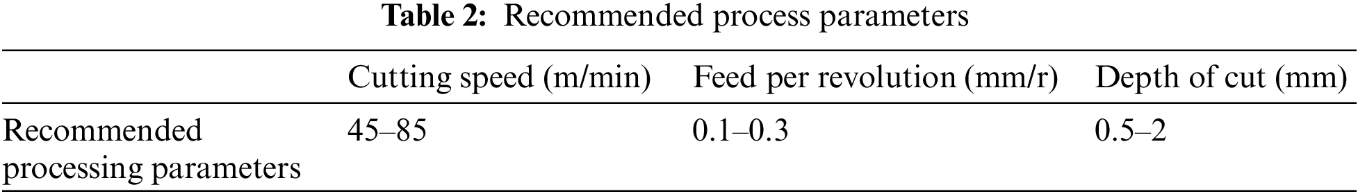
In actual production, the craftsman or operator usually selects the turning machining parameters based on the technical parameters of the machine tool and the range of machining parameters recommended by the turning tool manufacturer. In this paper, the above method will be used to select the turning machining parameters for the recommended machining parameters, and the recommended machining parameters are shown in Table 2.

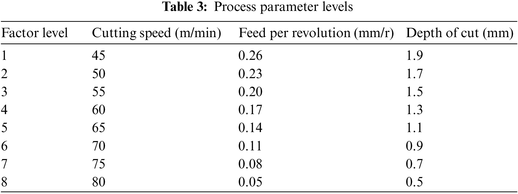
The values of the process parameters corresponding to each level in the equal probability orthogonal experimental design used in this paper are shown in Table 3.

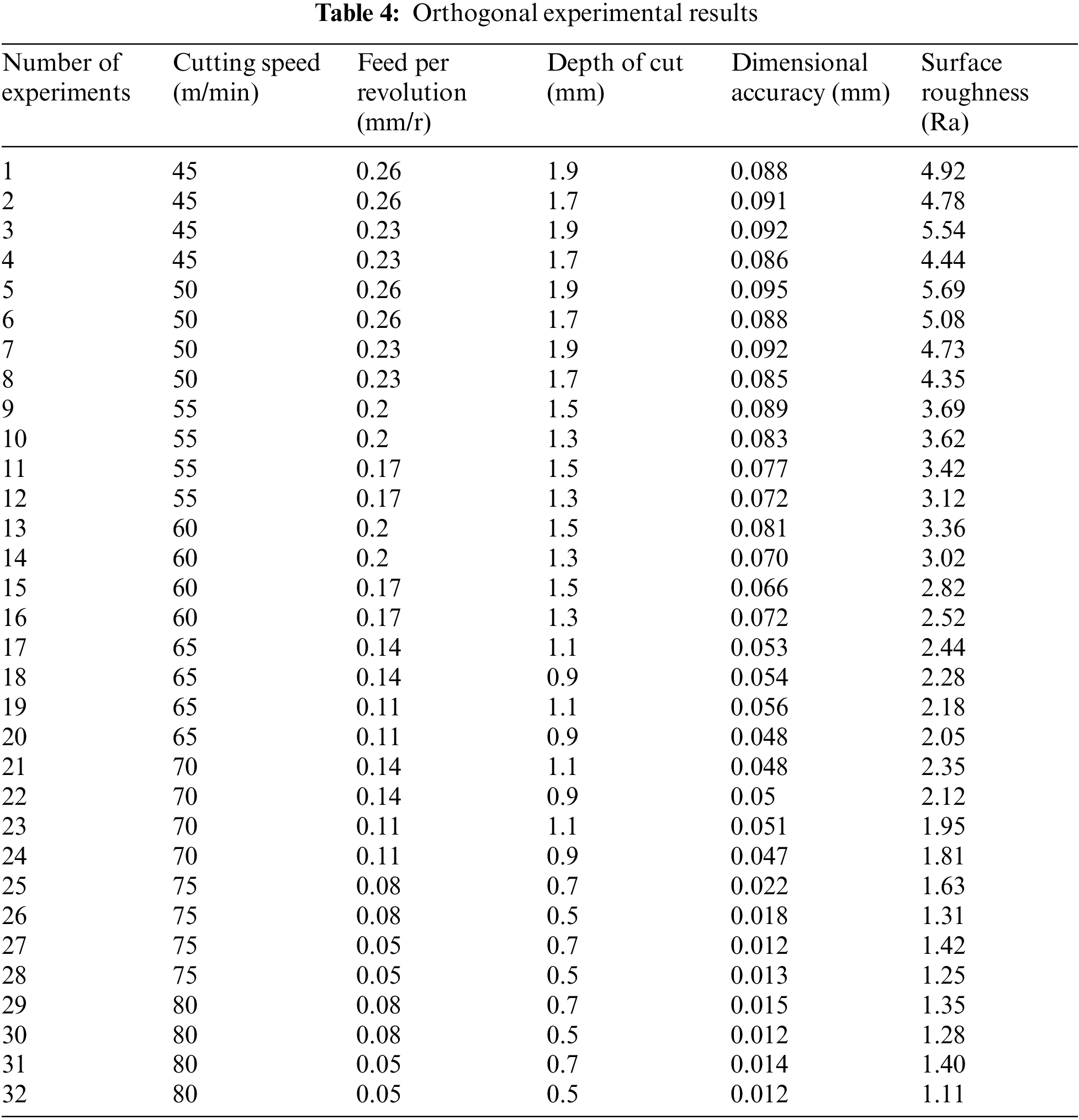
In this paper, a 3-factor 8-level equal-probability orthogonal experimental design with 32 experiments was used, that is, an L32 (8^3) orthogonal table was used. The process parameters, dimensional accuracy and surface roughness Ra for each group of experiments are shown in Table 4.

4.2 Determination of Model Structure and Parameters

4.2.1 Design of Model Structure

This paper establishes a neural network model NN1 with workpiece machining accuracy as the output and a neural network model NN2 with surface roughness Ra as the output. The input variables of both models are three key process parameters of turning machining: cutting speed (vc), feed per revolution (f) and depth of cut (ap). The model structure diagram is shown in Fig. 8. The 32 sets of data are randomly divided into two parts according to the ratio of 3:1, of which 22 sets of data are used as the training set data of the model and ten sets of data are used as the test set data of the model.

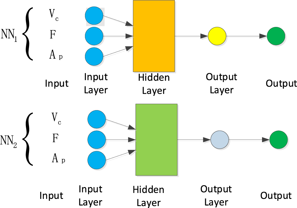
Figure 8: Two single-output neural network models, NN1 and NN2

4.2.2 Determination of the Number of the Hidden Layers

In order to determine the most suitable number of hidden layers, the Bp neural network models with different numbers of hidden layers are solved in this paper, and the results are shown in Figs. 9 and 10. From Figs. 9 and 10, it can be seen that the MSE of the test set is the lowest when the number of hidden layers is respectively 4 and 1 in the NN1 and NN2 network models. Although the MSE on the training set is lower when the number of hidden layers is 5 and 6, the MSE on the test set is higher, which indicates that too many hidden layers will make the model solution more complicated and thus, the phenomenon of overfitting will occur, leading to the weak generalization ability of the model. Therefore, in this paper, the number of hidden layers in the NN1 and NN2 network models is set to 4 and 1.

Figure 9: The influence of different hidden layers on MSE in NN1 network model

Figure 10: The influence of different hidden layers on MSE in NN2 network model

4.2.3 Number of the Hidden Layer Neurons

In Section 4.2.2 of this paper, the number of hidden layer layers in the NN1 and NN2 network models has been determined. However, in order to find a more suitable number of neurons for the hidden layer network, this paper has tested the effect of different numbers of neurons on the performance of the two network models. As can be seen from Figs. 11 and 12, in the NN1 model, when the number of neurons is 7, the MSE of the training and validation sets is the lowest. In the NN2 model, the MSE of both the training and validation sets is lowest when the number of neurons is 6. Therefore, the number of neurons in the hidden layer of the NN1 model is taken as 7, and the number of neurons in the hidden layer of the NN2 model is taken as 6.

Figure 11: The effect of different number of neurons on MSE in NN1 network model

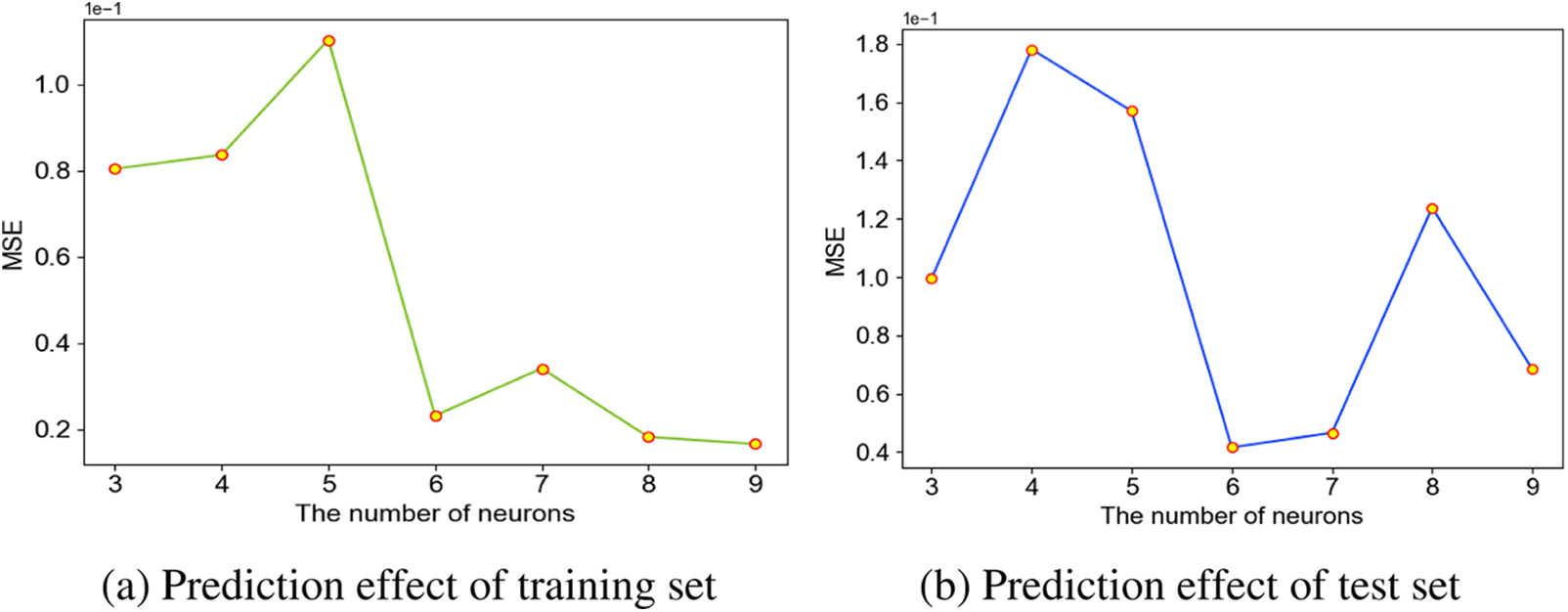
Figure 12: The effect of different number of neurons on MSE in NN2 network model

4.2.4 Model Prediction Results and Analysis

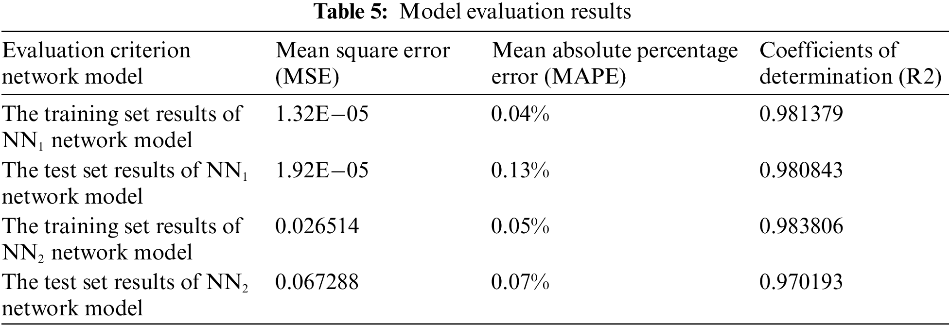
The regression performance of the models determines the accuracy of the prediction results. From the fitted curves Figs. 13 and 14 as well as Table 5, it can be seen that although there are some errors in the prediction results of the two models, the MSE and MAPE are low, while the R2 is high, which indicates that both models show good regression performance with high confidence.

Figure 13: NN1 network model training set and test set fitting results

Figure 14: NN2 network model training set and test set fitting results

4.2.5 Model Prediction Results and Analysis

The forecasting problem studied in this paper is a regression problem. In order to evaluate the accuracy of the prediction models, three model performance indicators—Mean Square Error (MSE), Mean Absolute Percentage Error (MAPE), and Determination Coefficient (R2), are used in this paper. The results of the model evaluation are shown in Table 5. From Table 5, it can be observed that although there are some errors in the prediction results of the two models, the Mean Square Error (MSE), Mean Absolute Percentage Error (MAPE) are both relatively small, and the determination coefficient (R2) is relatively high, which indicates that the two models have good performance in regression performance and have high confidence level.

4.2.6 Multi-Objective Function

In this case, the machining parameters in Table 1 are used as constraints. Meanwhile, to facilitate the observation of the graph, the optimization objective is transformed from maximizing the material removal rate to minimizing the reciprocal of the material removal rate (1/Q), and the multi-objective optimization model for this case is obtained after substitution into Eqs. (21)–(24) as shown in Eqs. (25)–(28).

min F(X)(25)

max 1Q(X)(26)

X=(vc,vf,ap)(27)

s.t{45≤vc≤850.1≤vf≤0.30.5≤ap≤2(28)

4.3 Optimization Results of the Bp-DWMOPSO Algorithm

The population initialization is set to 100; the maximum number of iterations is 50 [9]; the initial number of iterations is 0; the initial inertia weight is 0.4; and the final inertia weight is 0.9 [23]. The CNC turning machining parameter optimization problem is solved using the Bp-DWMOPSO algorithm, and the solved Pareto solution is shown in Fig. 14.

The traditional multi-objective particle swarm algorithm only solves the Pareto solution set according to the objective function requirements, as shown in Fig. 15(a). However, the Bp-DWMOPSO algorithm can satisfy both the objective function requirements and other performance indexes to solve the Pareto solution set, as shown in Fig. 15(b).

Figure 15: Comparison of Pareto solution sets for different algorithms

Although the number of solutions of the traditional multi-objective particle swarm algorithm is very large, many of the solutions do not necessarily satisfy the machining accuracy and surface roughness (Ra) requirements. The Pareto solution set obtained by the Bp-DWMOPSO algorithm not only meets the requirements of the objective function but also can meet the requirements of machining accuracy and surface roughness (Ra). And the results obtained are more in line with the actual machining and production requirements.

4.4 Decision Analysis by Analytical Hierarchy Process

This paper uses hierarchical analysis to select the optimal combination of cutting parameters among the six sets of machining parameter solutions obtained by the Bp-DWMOPSO method to obtain the optimal solution among the conflicting objectives of cutting maximum productivity and minimum production cost. The hierarchical analysis method uses level-by-level refinement and hierarchical comparison to determine the weights and finally synthesizes them according to the hierarchical structure to form the weights of each factor for the total objective [24].

In this paper, the six sets of solutions in Fig. 14 are used as the solution layer; the values obtained from the two objective functions are used as the criterion layer; the results of the identified optimal parameters are used as the objective layer. The pairwise comparison matrix of the solution layer to the criterion layer is:

F=(11111211/21411/2411/2531/21/41/41/5111/322211/31/3311/2321),1Q=(11/21/221221/21411/2411/2531/21/41/41/5111/322211/31/3311311)

The maximum eigenvalues are divided into 6.37 and 6.44. Take the weight vector W2 = [0.6, 0.4] T from the criterion layer to the target layer, whose consistency index CI is 0, respectively, and pass the consistency test. The eigenvectors corresponding to the maximum eigenvalues of F and 1/Q are found and normalized to obtain the weight vector W1 from the scheme layer to the criterion layer as:

w1=(0.280.280.470.480.470.490.110.110.290.340.620.58),w=w1×w2=(0.280.470.480.110.310.60)

Finally, according to the total ranking w of the hierarchy, the 6th group has the largest weight, and the obtained optimal parameters are shown in Table 6.

It can be seen that the selection of machining parameters has an important influence on the maximum production efficiency and the cost of CNC machining, and reasonable parameter selection has an important guiding significance for enterprise production.

5  Conclusion

As can be seen from the results of the turning machining case in Section 4, the Bp-DWMOPSO algorithm proposed in this paper fully combines the advantages of the Bp neural network’s learning ability, strong generalization ability and the particle swarm algorithm’s strong global search ability, which has achieved encouraging results. In this study, a reliable optimization model is established by collecting the data through equal probability orthogonal experiments and processing the data through the Bp-DWMOPSO algorithm. Eventually, the machining parameters are successfully optimized so that the requirements of machining accuracy and surface roughness can be met during the CNC turning machining process while taking into account the optimization of other key machining performance indexes. This not only significantly improves productivity and reduces cost but also ensures the quality and performance of the machined parts.

The results of this research show that with the help of the Bp neural network and the improved multi-objective particle swarm algorithm, more excellent results can be achieved in the field of CNC turning machining. This method can not only be widely used in the existing machining process but also provides a useful reference for the research of other similar multi-objective optimization problems.

Acknowledgement: Thank you to Shaofei Li and Yang Wang for their technical and equipment support.

Funding Statement: The authors received no specific funding for this study.

Author Contributions: Study conception and design: Jiang Li, Jiutao Zhao; data collection: Jiutao Zhao, Laizheng Zhu; analysis and interpretation of results: Qinhui Liu, Jiutao Zhao; draft manuscript preparation: Jinyi Guo, Weijiu Zhang. All authors reviewed the results and approved the final version of the manuscript.

Availability of Data and Materials: The data in this article are all from on-site actual processing, and the data results refer to Tables 3 and 4 in the article. If you have any other questions, you can send an email to 1245885036@qq.com Email for communication and discussion.

Conflicts of Interest: The authors declare that they have no conflicts of interest to report regarding the present study.

References

1. N. K. Sahu and A. B. Andhare, “Multi-objective optimization for improving machinability of Ti-6Al-4V using RSM and advanced algorithms,” Journal of Computational Design and Engineering, vol. 6, no. 1, pp. 1–12, 2019. [Google Scholar]

2. S. K. Shihab, J. Gattmah and H. M. Kadhim, “Experimental investigation of surface integrity and multi-objective optimization of end milling for hybrid Al7075 matrix composites,” Silicon, vol. 13, no. 5, pp. 1403–1419, 2020. [Google Scholar]

3. H. B. Xie and Z. J. Wang, “Study of cutting forces using FE, ANOVA, and BPNN in elliptical vibration cutting of titanium alloy Ti-6Al4V,” The International Journal of Advanced Manufacturing Technology, vol. 105, no. 12, pp. 5105–5120, 2019. [Google Scholar]

4. D. H. Tien, Q. T. Duc, T. N. Van, N. T. Nguyen, T. D. Duc et al., “Online monitoring and multi-objective optimization of technological parameters in highspeed milling process,” The International Journal of Advanced Manufacturing Technology, vol. 112, no. 9–10, pp. 2461–2483, 2021. [Google Scholar]

5. J. B. Li, Y. Y. Wu, P. Y. Li, X. F. Zheng, J. A. Xu et al., “TBM tunneling parameters prediction based on locally linear embedding and support vector regression,” Journal of Zhejiang University (Engineering Science), vol. 55, no. 8, pp. 1426–1435, 2021. [Google Scholar]

6. C. Y. Chen, J. Lu, K. Chen, Y. J. Li, J. Y. Ma et al., “Research on analytical model and DDQN-SVR prediction model of turning surface roughness,” Journal of Mechanical Engineering, vol. 57, no. 13, pp. 262–272, 2021. [Google Scholar]

7. C. Gong, T. Hu and Y. Ye, “Dynamic multi-objective optimization strategy of milling parameters based on digital twin,” Computer Integrated Manufacturing Systems, vol. 27, no. 2, pp. 478–486, 2021. [Google Scholar]

8. Q. L. Wang, P. Wei and X. H. Duan, “Multi-objective optimization of computer numerical control turning process parameters based on response surface method and artificial bee colony algorithm,” Industrial Engineering and Management, vol. 27, no. 3, pp. 117–126, 2022. https://doi.org/10.19495/j.cnki.1007-5429.2022.03.013 [Google Scholar] [CrossRef]

9. C. Wang, Y. Yang, H. B. Yuan and S. H. Wang, “NC cutting parameters multi-objective optimization based on hybrid particle swarm algorithm,” Modern Manufacturing Engineering, no. 3, pp. 77–82, 2017. https://doi.org/10.16731/j.cnki.1671-3133.2017.03.013 [Google Scholar] [CrossRef]

10. Q. L. Deng, J. Lu, Y. H. Chen, X. P. Liao, J. Y. Ma et al., “Optimization method of CNC milling parameters based on deep reinforcement learning,” Journal of Zhejiang University (Engineering Science), vol. 56, no. 11, pp. 2145–2155, 2022. [Google Scholar]

11. J. C. Osoriopinzon, S. Abolghasem, A. Maranon and J. P. Casasrodriguez, “Cutting parameter optimization of Al-6063-O using numerical simulations and particle swarm optimization,” The International Journal of Advanced Manufacturing Technology, vol. 111, no. 9–10, pp. 2507–2532, 2020. [Google Scholar]

12. H. P. Van, “Application of singularity vibration for minimum energy consumption in high-speed milling,” International Journal of Modern Physics B, vol. 35, no. 14n16, pp. 2140008, 2021. https://doi.org/10.1142/S0217979221400087 [Google Scholar] [CrossRef]

13. B. Li, X. T. Tian and M. Zhang, “Modeling and multi-objective optimization of cutting parameters in the high-speed milling using RSM and improved TLBO algorithm,” The International Journal of Advanced Manufacturing Technology, vol. 111, no. 7–8, pp. 2323–2335, 2020. [Google Scholar]

14. K. He, R. Tang and M. Jin, “Pareto fronts of machining parameters for trade-off among energy consumption, cutting force and processing time,” International Journal of Production Economics, vol. 185, pp. 113–127, 2017. [Google Scholar]

15. X. T. Wang and D. X. Cao, “Multi-strategy particle swarm optimization algorithm based on evolution ability,” Computer Engineering and Applications, vol. 59, no. 5, pp. 78–86, 2023. [Google Scholar]

16. W. B. Geng and Z. A. Zhou, “Research on improved particle swarm optimization for BLDCM speed control system,” Control Engineering of China, vol. 26, no. 9, pp. 1636–1641, 2019. [Google Scholar]

17. J. Wang, W. Li, J. Xu, Z. M. Wang and T. H. Wang, “Optimization on parameter of mask tooth mold by BP neural network,” Forging & Stamping Technology, vol. 48, no. 4, pp. 218–228, 2023. [Google Scholar]

18. J. Han, W. D. Shen, B. Y. Dong, S. Shao and N. N. Pang, “Optimization of milling parameters for annular thin walled parts based on improved particle swarm optimization,” Manufacturing Technology & Machine Tool, no. 6, pp. 133–138, 2023. [Google Scholar]

19. J. Sun, Y. R. Zheng, Z. M. Liu, J. Zhang, X. M. Xu et al., “Production process optimization of fresh Halloumi cheese based on BP neural network and genetic algorithm,” Food and Fermentation Industries, pp. 1–11, 2023. https://doi.org/10.13995/j.cnki.11-1802/ts.034871 [Google Scholar] [CrossRef]

20. C. A. C. Coello, G. T. Pulido and M. S. Lechuga, “Handling multiple objectives with particle swarm optimization,” IEEE Transactions on Evolutionary Computation, vol. 8, no. 3, pp. 256–279, 2004. [Google Scholar]

21. J. Q. Zhao, “Evolutionary multi objective optimization algorithms for learning and application,” P.H. dissertation, Xidian University, China, 2017. [Google Scholar]

22. Y. F. Zhang, Q. X. Zhu, H. R. Hou, G. L. Fu, H. G. Gu et al., “Cutting amount, cutting layer, material removal rate, basic concepts of cutting process,” in Metal Cutting Handbook, 4th ed., vol. 18, pp. 19–50, Shanghai, China: Shanghai Science & Technical Publishers, 2011. [Google Scholar]

23. Y. Bi, “Research on multi-objective problem based on particle swarm optimization,” M.S. dissertation, Harbin Engineering University, China, 2019. [Google Scholar]

24. S. Zeng, Z. Liu and J. Jiang, “Green remanufacturing comprehensive assessment method and its application of electromechanical products based on Fuzzy AHP,” Modern Manufacturing Engineering, no. 7, pp. 1–6, 2012. https://doi.org/10.16731/j.cnki.1671-3133.2012.07.029 [Google Scholar] [CrossRef]