
 Submit a Paper
 Propose a Special lssue
 Open Access
ARTICLE
Soil NOx Emission Prediction via Recurrent Neural Networks
1 Department of Mechanical Engineering, Iowa Technology Institute, University of Iowa, Iowa City, IA 52242, USA
2 Department of Chemical and Biochemical Engineering, Iowa Technology Institute, University of Iowa, Iowa City, IA 52242, USA
* Corresponding Author: Shaoping Xiao. Email:
Computers, Materials & Continua 2023, 77(1), 285-297. https://doi.org/10.32604/cmc.2023.044366
Received 28 July 2023; Accepted 15 September 2023; Issue published 31 October 2023
 View Full Text
 Download PDF
Abstract
This paper presents designing sequence-to-sequence recurrent neural network (RNN) architectures for a novel study to predict soil NOx emissions, driven by the imperative of understanding and mitigating environmental impact. The study utilizes data collected by the Environmental Protection Agency (EPA) to develop two distinct RNN predictive models: one built upon the long-short term memory (LSTM) and the other utilizing the gated recurrent unit (GRU). These models are fed with a combination of historical and anticipated air temperature, air moisture, and NOx emissions as inputs to forecast future NOx emissions. Both LSTM and GRU models can capture the intricate pulse patterns inherent in soil NOx emissions. Notably, the GRU model emerges as the superior performer, surpassing the LSTM model in predictive accuracy while demonstrating efficiency by necessitating less training time. Intriguingly, the investigation into varying input features reveals that relying solely on past NOx emissions as input yields satisfactory performance, highlighting the dominant influence of this factor. The study also delves into the impact of altering input series lengths and training data sizes, yielding insights into optimal configurations for enhanced model performance. Importantly, the findings promise to advance our grasp of soil NOx emission dynamics, with implications for environmental management strategies. Looking ahead, the anticipated availability of additional measurements is poised to bolster machine-learning model efficacy. Furthermore, the future study will explore physical-based RNNs, a promising avenue for deeper insights into soil NOx emission prediction.Keywords
Nomenclature
| GHG | Greenhouse gas |
| NOx | Nitrogen oxide |
| ANN | Artificial neural network |
| RNN | Recurrent neural network |
| DL | Deep learning |
| LSTM | Long short-term memory |
| GRU | Gated recurrent unit |
| MAE | Mean absolute error |
| RMSE | Root-mean-square deviation |
| R2 | Coefficient of determination |
| Symbol | |
| cell state | |
| cell input activation vector | |
| forget gate’s activation vecto | |
| hidden state | |
| reset gate vector | |
| time step | |
| input vector | |
| candidate activation vector | |
| update gate vector | |
| sigmoid function | |
| hyperbolic tangent function | |
The primary greenhouse gases (GHG), including CO2, N2O, O3, and CH4, can directly contribute to warming the earth’s atmosphere. Additionally, several other gases, especially nitrogen oxide (NOx = NO + NO2), can indirectly affect atmospheric warming because NOx emission contributes to the formation of tropospheric ozone (O3), a greenhouse gas. It has been shown that the increase of tropospheric O3 is the third-largest indirect radiative forcing of climate change [1]. On the other hand, NOx is an essential form of N trace gas that can be released from soils [2], especially fertilized soils. “Smart” agriculture is expected to minimize NOx emission for GHG mitigation while maximizing crop productivity under the constraints of NOx budget and energy consumption. Therefore, it is crucial to predict soil NOx emissions.
Several works have been done to model and estimate soil NOx emissions based on satellite observations and chemistry transport models (CTMs). Yienger et al. [3] developed a widely used algorithm to calculate global soil NOx emission in a temperature- and precipitation-dependent empirical model. Also, they considered synoptic-scale modeling of NOx “pulsing” caused by the wetting of dry soil and a biome-dependent scheme to estimate canopy recapture of NOx. Hudman et al. [4] presented a parameterization of soil NOx emissions and implemented this mechanistic model within a global chemical transport model (GEOS-Chem). In another work, Rasool et al. [5,6] developed a community multiscale air quality (CMAQ) model, introducing a mechanistic, process-oriented representation of soil emissions of N species. In addition, Wang et al. [7] improved soil NOx emission estimation using a new observation-based temperature response that led to better CTM simulation to match NOx observations.
Machine learning (ML), including supervised learning and reinforcement learning (RL), has boosted data-driven research in many domains, including materials science [8] and robotics. Verma et al. [9] proposed a fabricated heat exchanger using corrugated and non-corrugated pipes and estimated the heat transfer performance. They also modeled an artificial neural network (ANN) for predicting heat coefficient, Nusselt number, and Reynolds number.
Some data-driven models for estimating industrial NOx emissions have been reported. Xie et al. [10] studied low NOx emission control in power plants. They proposed a sequence-to-sequence dynamic prediction model to predict a future sequence of NOx emission from a selective catalytic reduction (SCR) system in the next time horizon. In another work, Yin et al. [11] developed a predictive model to predict the NOx emission concentration at the outlet of boilers under different operating conditions, including steady-state and transient-state conditions. Recently, Wang et al. [12] utilized datasets from the distributed control system of a coal-fired power plant and developed a hybrid model for accurate and reliable NOx concentration prediction. They employed complete empirical ensemble mode decomposition adaptive noise (CEEMDAN) to decompose the original historical data into a set of constitutive sequences. Then, a recurrent neural network (RNN) model was applied to predict each component separately before integrating the results for the final prediction.
Since NOx emission data is time series data, employing RNNs [13] in the prediction models as a data-driven approach is common. However, a naïve RNN suffers from issues of exploding and vanishing gradients. If the neural network’s weights are updated too quickly (i.e., exploding), a slight change in inputs may lead to high output variation. In contrast, if the weights are updated too slowly (i.e., vanishing), it may stop the network from learning anything new. An improved RNN, called long-short term memory (LSTM), was designed to resolve these issues [14] by learning long-term dependencies between the network’s input and output. In other words, an LSTM could remember both long-term and short-term patterns in the data. Therefore, the works mentioned above [10–12] in predicting industrial NOx emissions mostly utilized LSTMs for estimating industrial NOx emissions. On the other hand, Cho et al. [15] proposed a gated recurrent unit (GRU), maintaining the advantages of LSTM but with fewer gates, which could be trained faster.
While the studies mentioned earlier have predominantly concentrated on industrial NOx emissions, it is important to note that soil NOx emissions exhibit distinct patterns compared to their industrial counterparts. These patterns are characterized by observable NOx emission pulses [2]. The complexity of these patterns might present challenges for conventional RNNs to recognize effectively. This paper takes a pioneering step by introducing the concept of sequence-to-sequence RNN architectures, aiming to predict soil NOx emissions. This initiative is driven by the pivotal objective of understanding and mitigating the environmental impacts associated with such emissions. Remarkably, this study marks the first-ever attempt to leverage the potential of deep learning (DL) techniques for accurately predicting soil NOx emissions.
In addition to employing LSTM, we have developed and examined a novel neural network architecture that incorporates GRU cells with attention mechanisms [16]. It is worth noting that the proposed neural networks utilize an encoder-decoder model [10], where the encoder captures the information of all input elements into a fixed-length context vector. At the same time, the decoder learns contextual dependencies from the previous cells in the sequence. Therefore, this approach enhances the model’s understating of contextual information by allowing the decoder to assign weights to the context vector.
This paper is organized as follows: Section 2 describes the studied dataset and pre-processing. Section 3 describes LSTM and GRU and presents RNN architectures with the attention mechanism. The results are discussed in Section 4 with the studies of various input features, input series lengths, and training data sizes, followed by the conclusions and future works.
The data set we use in this study has been collected in Iowa by the Environmental Protection Agency (EPA). The EPA deploys around 360,000 sensors in the United States to monitor air quality, including criteria gases, particulates, meteorological, toxins, ozone precursors, and lead. Iowa has three monitoring locations: the city of Des Moines, the city of Davenport, and a forest located at 40°41’42.3” N, 92°00’22.7” W. It shall be noted that an essential factor in NOx emission is the soil nitrogen content. However, the soil nitrogen content can be significantly varied because of using nitrogen fertilizer, which depends on the agricultural management and farmer’s expertise. Therefore, we choose the data from the forest to avoid interference from human factors.
Each data sample consists of the following features: Latitude, Longitude, Date GMT, Time GMT, Sample Measurements, and Units of Measure. The measurements include air temperature (Fahrenheit), air moisture (percent relative humidity or RH) NOx emission, CO emission, O3 emission, and SO2 emission (parts per billion). While the dataset comprises numerous attributes, this study selectively narrows down the features to be utilized based on the available measurements. Notably, soil NOx emissions are prominently influenced by factors such as soil properties, soil temperature, and soil moisture [7]. Unfortunately, the current dataset lacks these specific details. Given that air temperature and moisture measurements can be correlated with soil temperature and humidity, our study opts to employ these two variables in conjunction with NOx emissions as the primary features.
The data has been collected every 60 min, i.e., one hour, since 1980. We select the data from January 2020 to September 2022 in this study. However, some data samples are missing due to sensor malfunctions. We try to use averaging or data imputation to replace the missing data, but they smear the NOx emission pulses. Since the whole data set is large enough, we drop the missing data and only keep the data consecutive for long periods to generate data sequences. Consequently, we have a total of 24096 data samples. Furthermore, we use data from 2020 to 2021, January to June 2022, and July to September 2022 as the training, validation, and testing datasets, respectively. Fig. 1 shows the testing set that has a total of 2116 data samples. It can be seen that there exist pulses that have been commonly observed in soil NOx emissions [2].
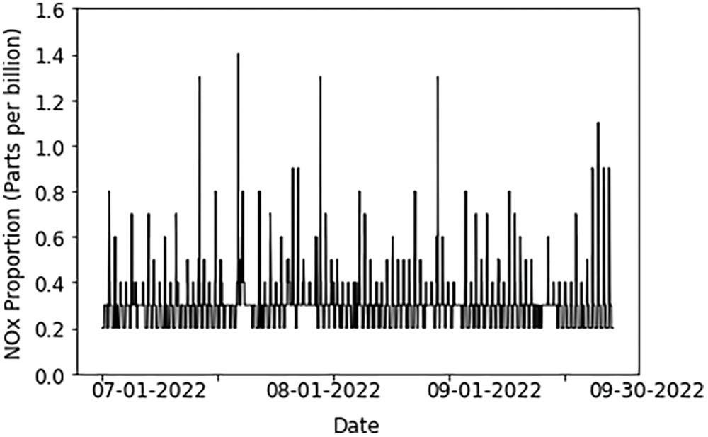
Figure 1: Testing data from July to September 2022
Recurrent Neural Networks are widely used in DL [16] to process sequential or time-series data. However, the naïve RNN has difficulty in capturing long-term dependencies [17] because the gradients tend to either vanish or explode during model training. Two main RNN variants, LSTM and GRU, have been developed to address this issue.
Long-short term memory was proposed initially by Hochreiter et al. [14] in 1997. Compared with the naïve RNN model, the LSTM model introduces a cell state calculated from the previous cell state and the current forget and input gates. Generally, an LSTM cell takes the input vector
where
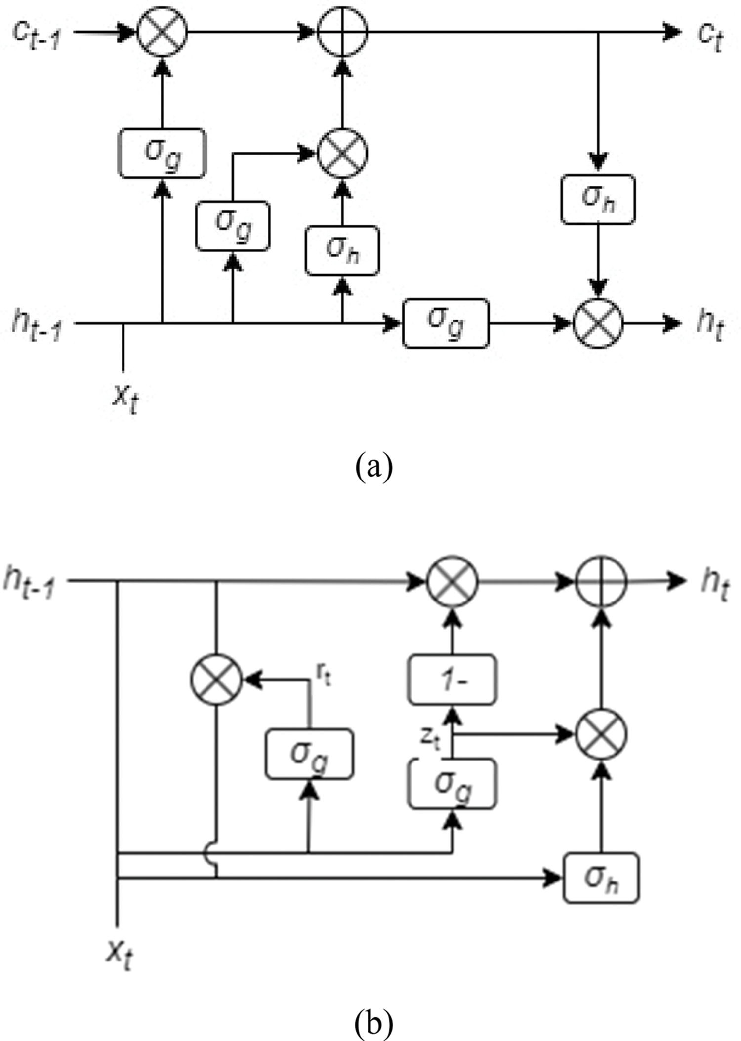
Figure 2: Basic structure of (a) a LSTM cell and (b) a GRU cell
The concept of GRU was proposed by Cho et al. [15] in 2014. Fig. 2b illustrates the network architecture of a GRU cell. Similar to LSTM, GRU also controls the information flow by “gates”. However, a GRU cell has one less gate than an LSTM cell, and it decomposes a gating signal into two components: a reset gate and an update gate. Since a GRU cell has only one forget gate without the output gate, it has fewer parameters and is more straightforward to implement than LSTM. In addition, it is easy to converge with limited data.
According to the principle of GRU, a typical mathematical model to process a data sequence can be presented below:
where
The RNN encoder-decoder is also used in this study. The encoder encodes the source time-series sequence to a fixed-length vector, and the decoder maps the vector back to the target time-series sequence [18]. The role of an encoder in the process is to handle the input sequence and condense its information into a singular vector, commonly referred to as the “context vector”. Specifically, the encoder operates repeatedly through the input sequence(s), adjusting its hidden state at each stage based on the current input and the preceding hidden state. Once the entire sequence has been processed, the final hidden state of the RNN encoder is utilized as the context vector, which intends to encapsulate the input sequence’s information.
The decoder takes the context vector generated by the encoder(s) and transforms it into the target sequence. The initial hidden state of the decoder is set to be the context vector from the encoder. The decoder then generates the output sequence in a step-by-step manner, in which each step takes the previous hidden state, i.e., the previously generated output [15], as the input.
3.4 Model Architecture and Training
Initially, we considered three input features in the DL models, including past and future air temperature, past and future air moisture, and past NOx emissions, to predict future NOx emissions. In order to reduce the interference of the NOx pulse on the prediction accuracy of the model, we used four days of data as a training unit to forecast the coming NOx data in the next six hours. Therefore, the temperature and moisture sequences consist of 96 past timesteps and 6 future timesteps, and the input NOx emission sequence encompasses 96 past timesteps. The output sequence, i.e., the forecasted future NOx emission sequence, has 6 timesteps. It shall be noted that the timestep is one hour in this study.
The architecture of our model is depicted in Fig. 3. The generated DL models consist of a single hidden layer with 32 neurons (or units) representing the memory cells in the LSTM or GRU structure. It shall be noted that we utilize grid search to find the optimal neural network. Some other neural networks with more hidden layers and neurons can achieve similar performance but longer training times. Since the lengths of temperature and moisture sequences differ from the length of the NOx emission sequence in the input, the models include two encoders and one decoder, as described in Section 3.3. We also implement an attention mechanism [19]. The reason for using attention is that it allows the models to focus on different parts of the input for each step of the output sequence, thereby improving their ability to capture dependencies between inputs and outputs. We also investigate the performance of DL models that use past NOx emissions as the only input feature. In such an instance, the encoders and decoders are not necessary.
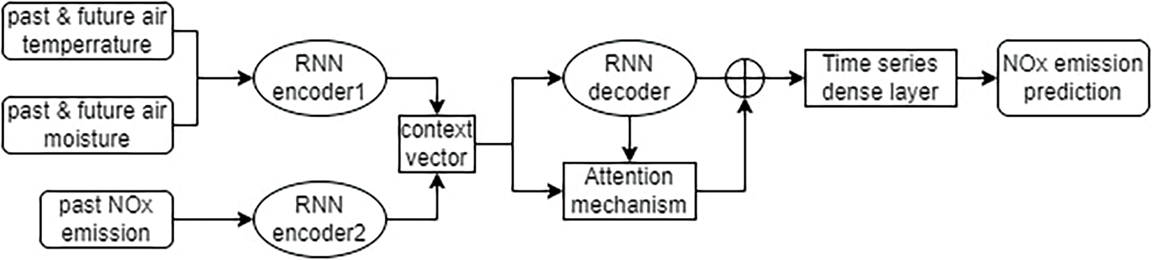
Figure 3: The sequence-to-sequence-attension model architecture
We utilize the Keras library in conjunction with the Adam optimizer to train neural networks using a learning rate of 0.002 and a batch size of 128. The training processes are conducted over 1000 epochs. In this study, we conduct the model training and testing using Python as the programming language, hosted on a machine equipped with an Intel Core i7-12700 K processor, NVIDIA GeForce RTX 3070 Ti graphics card, and 32 GB RAM.
In this section, we assess the performance of GRU and LSTM on the testing dataset and select the model with better performance as our major experimental model. Then, we investigate the performance of DL models using different input features and sequence lengths. We also study the impact of training dataset size on the DL model performance. The mean absolute error (MAE), the root-mean-square deviation (RMSE), and the coefficient of determination (R2) are used to evaluate the model performance as different look-back values. The smaller the MAE and RMSE values, the more accurate the forecast result is. On the other hand, R2 = 1 means the perfect fitting.
It shall be noted that future temperature and moisture must be predicted for the testing data before evaluating model performances. Taking temperature prediction as an example, a simple LSTM model is employed to take the temperature within the past 96 h as the input and predict the temperature in the next 6 h. The predicted temperatures of the part of the testing data (from July 01, 2022 to July 31, 2022) are compared to the actual ones in Fig. 4. We also use support vector machines for air temperature and moisture predictions, and the models perform similarly well.
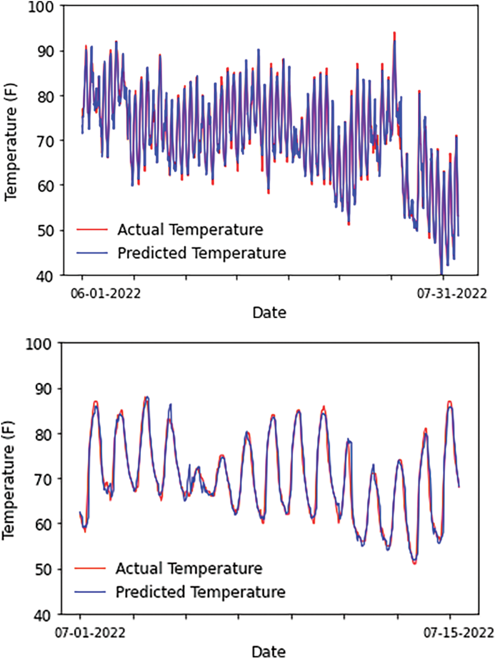
Figure 4: The prediction of temperatures as part of the testing dataset. The top panel shows two months of the results, while the bottom panel provides a zoom-in view of two weeks
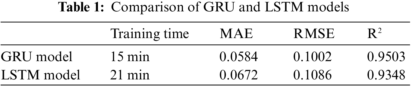
After predicting the future temperature and moisture, we train LSTM and GUR models to predict NOx emission. Fig. 5 illustrates the prediction from the GRU model, compared to the actual output of the testing dataset. It can be seen that the GRU model can efficiently recognize the NOx emission patterns, especially predicting the NOx emission pulses. The LSTM model also demonstrates good performance, but the results are worse than the ones of the GRU models. After comparing the training time and the MAE, RMSE, and R2 results, as shown in Table 1, we decide to use the GRU model for other studies in this paper.
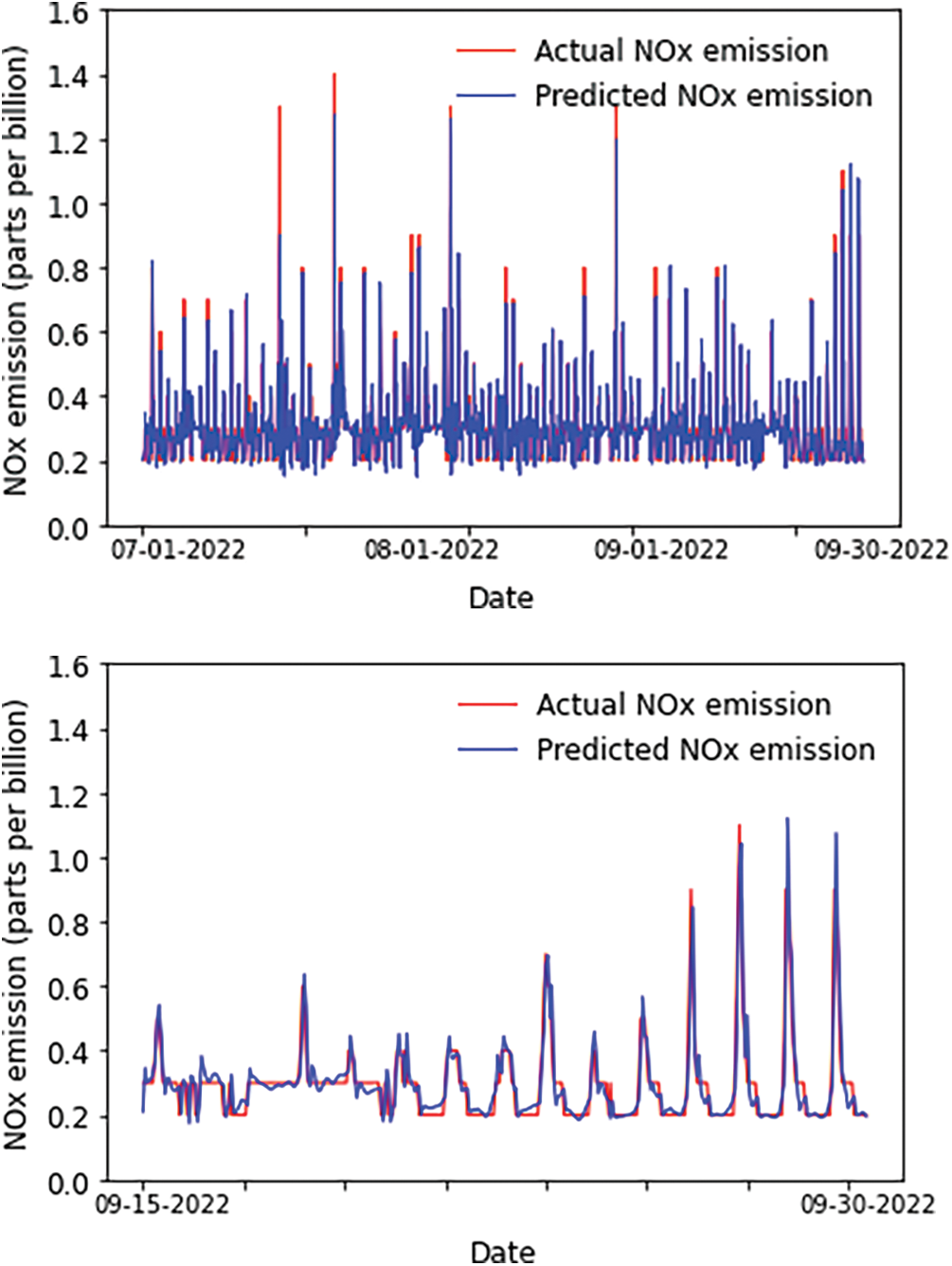
Figure 5: The prediction of NOx emission in the testing dataset using the GRU sequence-to-sequence attention model
The original model uses past and future air temperatures, past and future air moisture, and past NOx emissions as input features. The lengths of input air temperature and moisture sequences are 102 h, including the past 96 h (i.e., four days) and the future 6 h. Correspondingly, the length of the input NOx emission sequence is 96 h from the past four days only. In addition, the original model forecasted NOx emission in the next 6 h. We also employ the same GRU model to predict NOx emission for the next 24 h. The MAE, RMSE, and R2 are 0.0522, 0.1053, and 0.90, respectively, similar to the results in Table 1.
We extend the original model to two variants using different input features. The first model uses air temperature and moisture only, while the second model takes past NOx emission as the only input. Both models do not use encoders because the input features have the same sequence length. We also vary the input sequence length considering the past 3 days (i.e., 72 timesteps or hours) and the past 7 days (i.e., 168 timesteps or hours) to investigate model performances. The same testing dataset described above is utilized, and the comparisons are listed in Table 2. Here, we present the NOx emission predictions generated by the DL model using air temperature and moisture as the sole inputs, as depicted in Fig. 6. The comparison involves the actual outputs of the testing data recorded between September 15 and 30, 2022. While the emission pattern is largely recognizable, it is important to note that there are significant errors in predicting the magnitudes of NOx emission pulses. On the other hand, Table 2 also shows that the NOx emission history plays an essential role in NOx emission predictions. Even taking NOx emission history as the only input, the model performances are acceptable, compared to the original model, and much better than the DL models that use air temperature and moisture as the inputs.
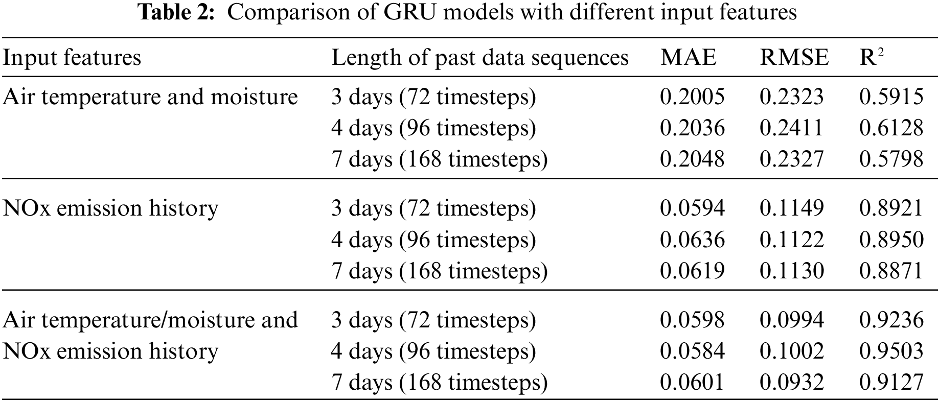
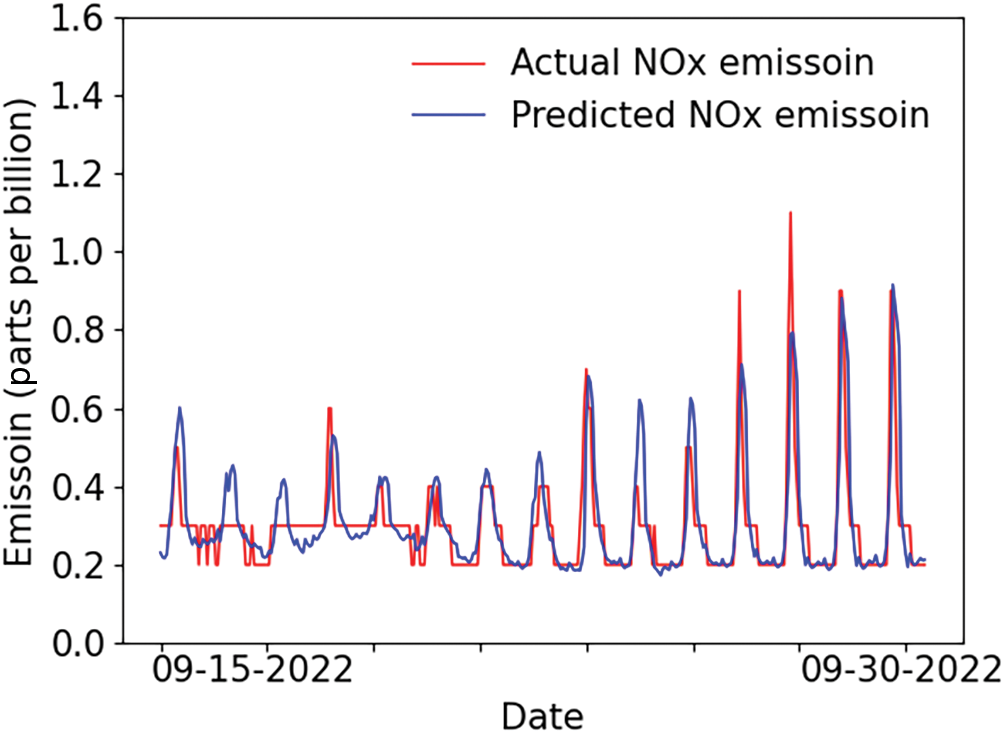
Figure 6: The prediction of NOx emission in the testing dataset using air temperature and moisture as the only inputs
Initially, we use the data of 2020 and 2021, i.e., 24 months, as the training set. In this study, we also investigate the size effect of the training set on model performance. Two different data sizes are utilized for the training sets: 12 months (the year 2021 only) and 6 months (June to December 2021). The validation and testing sets remain the same, as described in Section 3. After training, the DL models are employed to predict NOx emission in the next 6 h in the testing set, and the results (MAE, RMSE, and R2) are calculated in Table 3. The R2 score of the DL model, trained using 12 months of data, notably reaches a high value of 0.8269. The predictive capability of this DL model is visually evident in Fig. 7, where it demonstrates accurate forecasting of NOx emission pulses, akin to the original model showcased in Fig. 5. As a result, we can confidently infer that employing a 12-month dataset for training yields satisfactory outcomes.
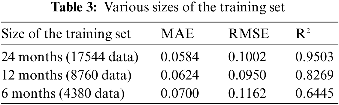
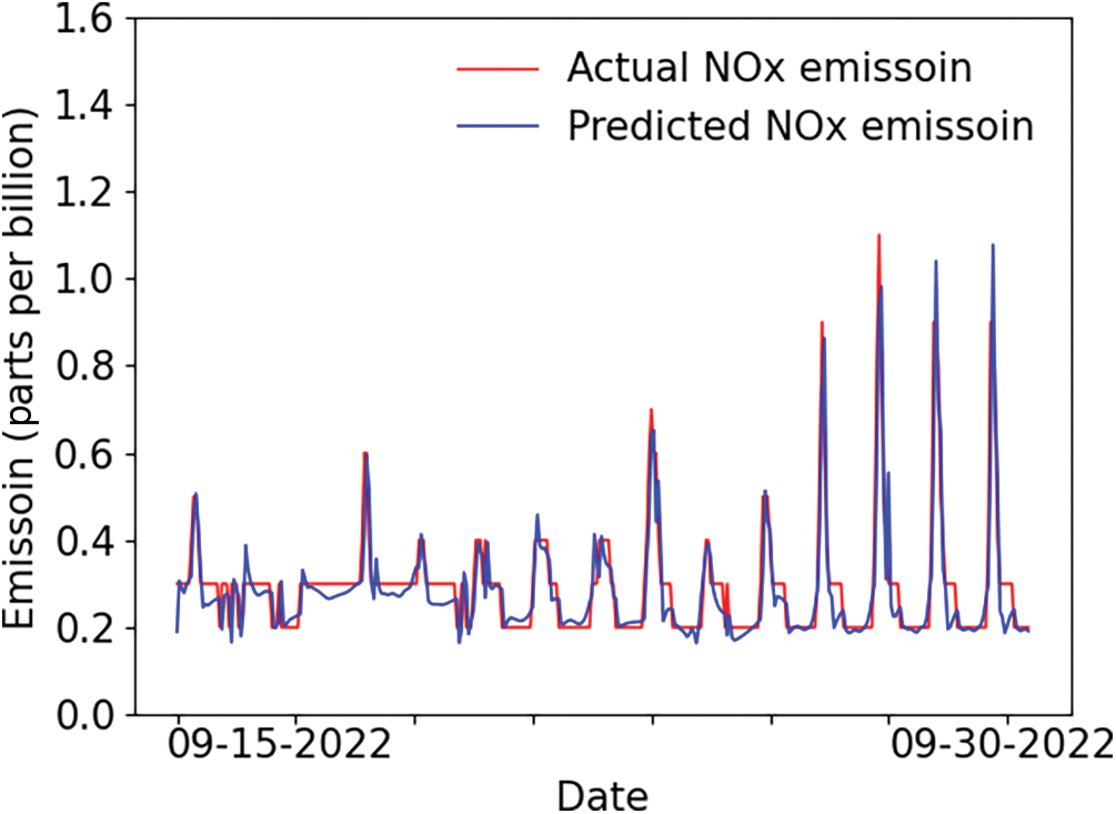
Figure 7: The prediction of NOx emission in the testing dataset using 12 months of data for training
In this paper, we have introduced sequence-to-sequence attention neural network architectures tailored for soil NOx emission prediction. Through a thorough comparison between the GRU and LSTM models, we have demonstrated that the GRU model consistently outperforms the LSTM counterpart in terms of forecasting accuracy. Moreover, our investigations into different input features and various dataset sizes have yielded valuable insights. Notably, we have found that the model can achieve commendable accuracy when trained on a 12-month data subset. A significant observation from our research is the dominant role of NOx emission history in predicting future emissions. Our DL model, which exclusively relies on past NOx emission records as input, has produced credible predictions, even in the absence of air temperature and moisture data. This underscores the pivotal importance of historical emission trends in shaping the accuracy of our predictions.
In our ongoing research, we will endeavor to expand our dataset to encompass fertilized soil data, recognizing the pivotal role of nitrogen content in influencing NOx emissions. While our present study has suggested that air temperature and moisture exhibit less significance as input features compared to NOx emission history, we remain committed to delving deeper into the influence of soil temperature and moisture. This exploration will be undertaken as new data sources become available, potentially enriching our understanding of these factors.
Our future efforts will also involve incorporating data related to irrigation and precipitation. We believe that this supplementary information can significantly enhance our model’s predictive capabilities, particularly in capturing NOx emission pulses with heightened precision and accuracy. As we expand the number of available features, we will adopt feature selection strategies such as leveraging Pearson correlation coefficients to ascertain the degree of inter-feature correlation [20]. Moreover, we are excited about the prospect of crafting a hybrid model that merges the strengths of chemical transport models with data-driven approaches like physics-informed neural networks. This innovative fusion offers an alternative avenue to improve our predictive accuracy. By integrating these enhancements and novel techniques, we anticipate the development of a more refined predictive model for soil NOx emissions, with a heightened focus on capturing intricated NOx pulse patterns.
Acknowledgement: Not applicable.
Funding Statement: The authors received support from the University of Iowa Jumpstarting Tomorrow Community Feasibility Grants and OVPR Interdisciplinary Scholars Program for this study. Z. Wang and S. Xiao received support from the U.S. Department of Education (E.D. #P116S210005). Q. Wang and J. Wang acknowledge the support from NASA Atmospheric Composition Modeling and Analysis Program (ACMAP, Grant #: 80NSSC19K0950).
Author Contributions: Study conception and design: Z. Wang, S. Xiao, Q. Wang, J. Wang; data collection: Z. Wang; analysis and interpretation of results: Z. Wang, S. Xiao, C. Reuben, J. Wang; draft manuscript preparation: Z. Wang, S. Xiao, J. Wang. All authors reviewed the results and approved the final version of the manuscript.
Availability of Data and Materials: The dataset used in this study can be downloaded from the following link: https://aqs.epa.gov/aqsweb/airdata/download_files.html.
Conflicts of Interest: The authors declare that they have no conflicts of interest to report regarding the present study.
References
1. G. Schaufler, B. Kitzler, A. Schindlbacher, U. Skiba, M. A. Sutton et al., “Greenhouse gas emissions from European soils under different land use: Effects of soil moisture and temperature,” European Journal of Soil Science, vol. 61, no. 5, pp. 683–696, 2010. [Google Scholar]
2. P. Y. Oikawa, C. Ge, J. Wang, J. R. Eberwein, L. L. Liang et al., “Unusually high soil nitrogen oxide emissions influence air quality in a high-temperature agricultural region,” Nature Communications, vol. 6, no. 1, pp. 1–10, 2015. [Google Scholar]
3. J. J. Yienger and H. Levy, “Empirical model of global soil-biogenic NOχ emissions,” Journal of Geophysical Research: Atmospheres, vol. 100, no. D6, pp. 11447–11464, 1995. [Google Scholar]
4. R. C. Hudman, N. E. Moore, A. K. Mebust, R. V. Martin, A. R. Russell et al., “Steps towards a mechanistic model of global soil nitric oxide emissions: Implementation and space based-constraints,” Atmospheric Chemistry and Physics, vol. 12, no. 16, pp. 7779–7795, 2012. [Google Scholar]
5. Q. Z. Rasool, R. Zhang, B. Lash, D. S. Cohan, E. J. Cooter et al., “Enhanced representation of soil NO emissions in the community multiscale air quality (CMAQ) model version 5.0.2,” Geoscientific Model Development, vol. 9, no. 9, pp. 3177–3197, 2016. [Google Scholar]
6. Q. Z. Rasool, J. O. Bash and D. S. Cohan, “Mechanistic representation of soil nitrogen emissions in the community multiscale air quality (CMAQ) model v 5.1,” Geoscientific Model Development, vol. 12, no. 2, pp. 849–878, 2019. [Google Scholar]
7. Y. Wang, C. Ge, L. Castro Garcia, G. D. Jenerette, P. Y. Oikawa et al., “Improved modelling of soil NOx emissions in a high temperature agricultural region: Role of background emissions on NO2 trend over the US,” Environmental Research Letters, vol. 16, no. 8, pp. 84061, 2021. [Google Scholar]
8. Y. Zhao, “Understanding and design of metallic alloys guided by phase-field simulations,” npj Computational Materials, vol. 9, pp. 94, 2023. [Google Scholar]
9. T. N. Verma, P. Nashine, D. V. Singh, T. S. Singh and D. Panwar, “ANN: Prediction of an experimental heat transfer analysis of concentric tube heat exchanger with corrugated inner tubes,” Applied Thermal Engineering, vol. 120, pp. 1359–4311, 2017. [Google Scholar]
10. P. Xie, M. Gao, H. Zhang, Y. Niu and X. Wang, “Dynamic modeling for NOx emission sequence prediction of SCR system outlet based on sequence to sequence long short-term memory network,” Energy, vol. 190, pp. 116482, 2020. [Google Scholar]
11. G. Yin, Q. Li, Z. Zhao, L. Li, L. Yao et al., “Dynamic NOx emission prediction based on composite models adapt to different operating conditions of coal-fired utility boilers,” Environmental Science and Pollution Research, vol. 29, no. 9, pp. 13541–13554, 2022. [Google Scholar] [PubMed]
12. X. Wang, W. Liu, Y. Wang and G. Yang, “A hybrid NOx emission prediction model based on CEEMDAN and AM-LSTM,” Fuel, vol. 310, pp. 122486, 2022. [Google Scholar]
13. J. Schmidhuber, “Deep learning in neural networks: An overview,” Neural Networks, vol. 61, pp. 85–117, 2015. [Google Scholar] [PubMed]
14. S. Hochreiter and J. Schmidhuber, “Long short-term memory,” Neural Computation, vol. 9, no. 8, pp. 1735–1780, 1997. [Google Scholar] [PubMed]
15. K. Cho, B. van Merriënboer, C. Gulcehre, D. Bahdanau, F. Bougares et al., “Learning phrase representations using RNN encoder-decoder for statistical machine translation,” in Proc. of 2014 Conf. on Empirical Methods in Natural Language Processing, Doha, Qatar, pp. 1724–1734, 2014. [Google Scholar]
16. Y. Lecun, Y. Bengio and G. Hinton, “Deep learning,” Nature, vol. 521, no. 7553, pp. 436–444, 2015. [Google Scholar] [PubMed]
17. Y. Bengio, P. Simard and P. Frasconi, “Learning long-term dependencies with gradient descent is difficult,” IEEE Transactions on Neural Networks, vol. 5, no. 2, pp. 157–166, 1994. [Google Scholar] [PubMed]
18. I. Sutskever, O. Vinyals and Q. V. Le, “Sequence to sequence learning with neural networks,” in NIPS’14: Proc. of the 27th Int. Conf. on Neural Information Processing Systems, Montreal, Canada, pp. 3104–3112, 2014. [Google Scholar]
19. D. Bahdanau, K. H. Cho and Y. Bengio, “Neural machine translation by jointly learning to align and translate,” in Proc. of the 3rd Int. Conf. on Learning Representations, San Diego, CA, USA, 2015. [Google Scholar]
20. Q. Guo, X. Xu, X. Pei, Z. Duan, P. Liaw et al., “Predict the phase formation of high extropy alloys by compositions,” Journal of Materials Research and Technology, vol. 22, pp. 3331–3339, 2023. [Google Scholar]
Cite This Article
 Copyright © 2023 The Author(s). Published by Tech Science Press.
This work is licensed under a Creative Commons Attribution 4.0 International License , which permits unrestricted use, distribution, and reproduction in any medium, provided the original work is properly cited.
 Downloads
 Citation Tools