Electroencephalography (EEG) Based Neonatal Sleep Staging and Detection Using Various Classification Algorithms

1  Introduction

Sleep is an anatomical action that is usually found in all species of animal. Approximately one third of a person’s life is dedicated to sleep [1]. A healthy life requires sleep, as sleep deprivation leads to severe medical complications, such as cognitive impairment and death. Sleep is a naturally reverting state of the brain and body. It is characterized by diversified consciousness, comparatively inhibited sensory activity, lessened muscle activity and interference with almost all voluntary muscles, and reduced interactions with the surroundings. Neonates consume their time mostly relaxing in a sleep condition.

Now the question arises that why sleep is important to a baby’s development? Eliot et al. in 1999 proposed that in one second a baby makes up to 1.8 million new neuronal connections in the brain, and what a baby feels, sees, hears, and smells determines which of these connections will remain [2]. Thiedke et al. in 2001 researched that infants spend most of their time asleep and that a notable proportion of sleep is in the processing Rapid eye movement (REM) stage [3]. The authors in [4,5] suggested that sleep is necessary during the early development of a baby’s brain and body. Clinically, the main symbol of brain evolution in infants is Sleep-Wake Cycle (SWC) [6,7]. SWC basically demonstrates 24-h everyday sleep-wake pattern. It consists of normally 16 h of wakefulness in the daytime and the remaining 8 h of sleep at night-time [6,7]. In particular, neonatal sleep should be preserved and encouraged in a neonatal intensive care unit (NICU). Infants can suffer from many sleep-related serious problems, including Sleep Apnea, Infantile Spasms, Blindness, Irregular sleep-wake cycle, non-24-h sleep-wake cycle, Down syndrome, and Nighttime Sleep Disturbances [8]. Neonatal sleep staging is also important to reduce the risk of sleep-related infant deaths which are tragic and devastating outcomes during sleep [9]. These deaths are categorized into two main types: Infant Death Syndrome (SIDS): SIDS is the sudden, unpredictable death of a neonate aged less than one year, often while sleeping, and its exact cause is unknown. Accidental Suffocation or Strangulation in Bed (ASSB): This occurs when something in the sleep environment blocks an infant’s airway during sleep. It is the most common cause of death for infants under one year. Polysomnography (PSG) is basically a sleep study and a thorough test used to detect sleep and sleep problems [10]. The polysomnography method records brain waves, heart rate, respiration, oxygen level in the blood, and eye and leg movements during sleep. The electrical activity in the brain is evaluated by using an Electroencephalogram (EEG) and the process is called Electroencephalography. With the help of electrical impulses, brain cells communicate with each other. Brain wave patterns are tracked and recorded by an EEG. In the past, researchers have illustrated the practicability of automatic sleep classification algorithms with PSG signals, out of which EEG is contemplated as the most authentic signal for both mature people [11–13] and neonates [14–16].

There exist conflicting EEG patterns for infants and mature people. A comparison of the EEG patterns of adults and infants will reveal that infant’s EEG patterns have smaller amplitudes. Within the first three years of an infant’s life, different maturity changes happen [17]. So, for automated neonatal sleep classification, several algorithms have been developed that are based on EEG. Most of the already existing algorithms designed for EEG-based neonatal sleep staging do not distinguish ‘wake’ as a distinct state. While other algorithms classify sleep stages according to different characteristics of EEG signals, including Low Voltage Irregular (LVI), Active Sleep II (AS II), High Voltage Slow (HVS) and Trace Alternant (TA)/Trace Discontinue (TD) [16,18–20]. The process of brain maturation starts during AS and wakes.

Main contributions: The main aim of this research is to design such an algorithm that basically avoids the jumbling of multiple sleep stages by categorizing wake and sleep as totally different stages and improving the accuracy of [21]. Therefore in this paper, autoML-based 18 different algorithms: Random Forest, Adaboost Random Forest, Decision Tree (DT), Adaboost DT, Support Vector Machine (SVM), Adaboost SVM, Gaussian Naive Bayes (GNB), Quadratic Discriminant Analysis (QDA), Linear Discriminant Analysis (LDA), KNeighbours (KN), Ensemble Extra Tree Classifier (ETC), ETC with GridSearchCV, Multi-Layer Perceptron (MLP), Voting Classifier (Logistic Regression (LR), DT Classifier, Support Vector Classifier (SVC)), Stacking Classifier (KN, LR, MLP, Random Forest), Gradient Boosting (GB), Extreme Gradient Boosting (XGB), and LR are presented for the categorization of sleep-wake. Among these 18 different AutoML-based algorithms, this study also aimed to identify the algorithm that achieved the highest accuracy. This research is basically comprised of three parts: (1) feature extraction (3) autoML based hyperparameter tuning and (2) classification of sleep and wake. Total twelve numbers of features were extracted from multichannel EEG data. Then one by one all estimators were applied for training and testing. Furthermore, a comparison is made between the proposed methodology and reference [21] through the use of the same dataset, resulting in an improvement in accuracy and kappa.

The rest of the article is arranged as follows: Section 2 presents the related work. Methodology is proposed in Section 3. The classification results using the proposed methods are reported in Section 4 and discussed in Section 5. The conclusion of the research is presented in Section 6. Furthermore, Section 7 includes future recommendations.

2  Related Work

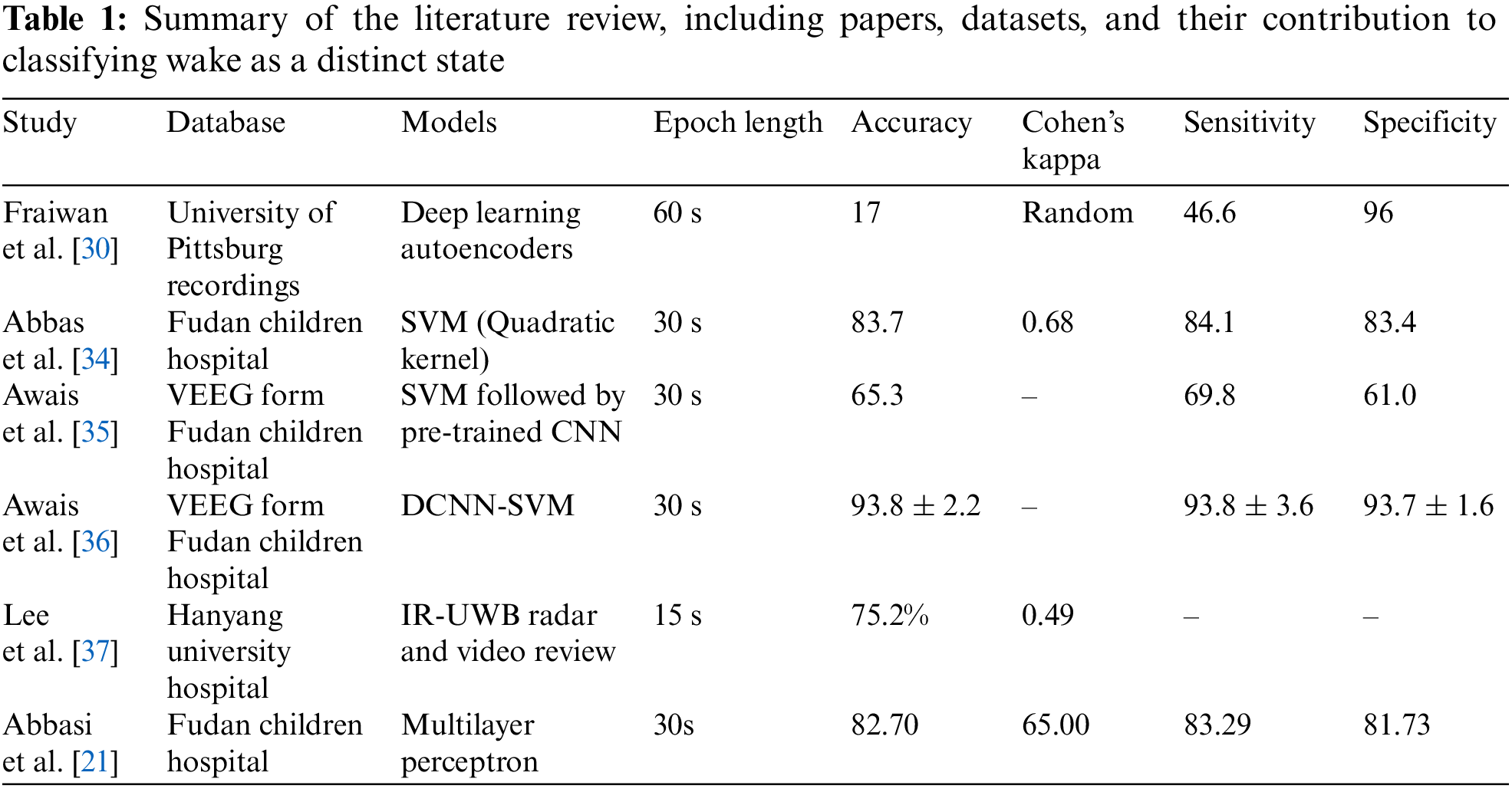
The first application of EEG, based on the study of human sleep behavior, was made in 1937 by Loomis et al. [22]. Loomis’s new research has resulted in numerous algorithms for classification of adult sleep using deep and machine learning [14–16,23–30]. Using least squares support vector machine (LS-SVM) classifiers, De et al. proposed an advanced model to estimate the neonate’s Postmenstrual Age (PMA) during Quiet Sleep (QS) and to classify sleep stages [28]. Cluster-based Adaptive Sleep Staging (CLASS) was designed by Dereymaeker et al. for automatic QS detection and to highlight its role in brain maturation [14]. Based on EEG data, the authors in [15] developed a SVM algorithm that tracks neonatal sleep states and identifies QS with an efficiency of 85%. On the basis of multi-channel EEG recordings, Pillay et al. developed a model to automatically classify neonate’s sleep using HMM (Hidden Markov Models) and GMM (Gaussian Mixture Models). They found HMMs superior to GMMs, with a Cohen’s Kappa of 0.62. Later, they used an algorithm based on a Convolutional Neural Network (CNN) to classify 2 and 4 states of sleep [29]. For classifying QS with an enhanced Sinc-based CNN based on EEG data, another study achieved a mean Kappa of 0.77 ± 0.01 (with 8-channel EEG) and 0.75 ± 0.01 (with one bipolar channel EEG) [31]. Using publicly available single-channel EEG datasets, Rui et al. classified neonates’ sleep patterns into Wake, N1, N2, N3, and REM [32]. Classification was performed using the MRASleepNet module. Hangyu et al. designed MS-HNN in 2023 for the automatic classification of newborns’ sleep using two, four, and eight channels [33]. In order to extract more features from sleep signals involving temporal information, they employed multiscale convolutional neural networks (MSCNN), squeeze-and-excitation blocks (SE) and temporal information learning (TIL). However, none of the algorithms above included the waking state as a separate state in infants. Table 1 summarizes the literature review, including papers, datasets, and their contribution to classifying wake as a distinct state.

3  Methodology

The complete description of the designed AutoML-based estimators is presented in this section. Fig. 1 illustrates the step-wise flowchart of the proposed methodology. The method can be further elaborated in the following steps.

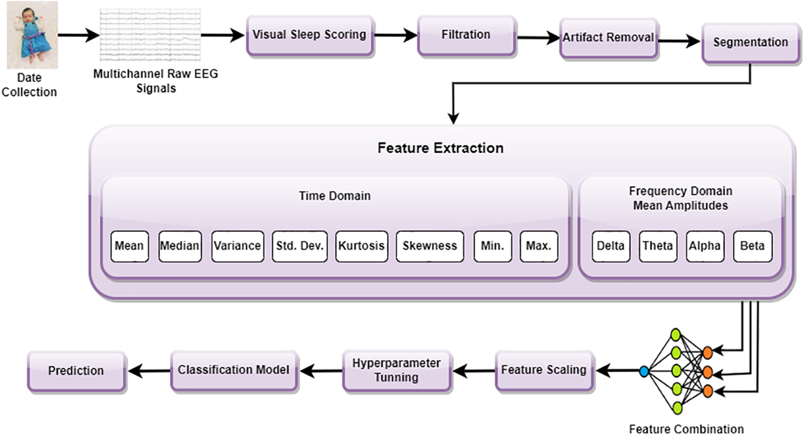
Figure 1: Step-wise flowchart of the proposed methodology

3.1 Dataset

EEG was recorded from 19 infants in the NICU at a Children’s Hospital of Fudan University (CHFU), China. The Research Ethics Committee of the CHFU approved the study (Approval No. (2017) 89). Generally, a neonate was kept under observation for 2 h and data was recorded. At least one sleep cycle was observed during these 2 h. A complete 10–20 electrode installation system includes: “FP1–2”, “F3–4”, “F7–8”, “C3–4”, “P3–4”, “T3–4”, “T5–6”, “O1–2”, and “Cz” (17 electrodes). Depending on where the electrode is placed on the brain, a letter will indicate what lobe or location is being assessed. Pre-frontal, frontal, temporal, parietal, occipital, and center, respectively, are represented by the letters FP, F, T, P, O, and C. From 19 EEG recordings, 15 contain all the electrodes specified, except for “T5–6”, “F7–8” and “O1–2” (11 electrodes). For the remaining four recordings, “T5–6”, “F7–8”, “Cz” and “O1–2” were not recorded, resulting in 10 electrodes being included [21]. The multichannel EEG was obtained using the NicoletOne EEG system. Fig. 2 shows the electrode locations for the 10 electrodes used in this study based on the 10–20 system. Note that NZ indicates the nose’s root and IZ indicates protuberance.

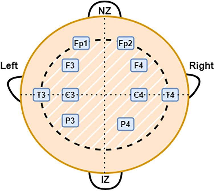
Figure 2: Electrode locations for the 10 electrodes used in this study based on the 10–20 system

3.2 Visual Sleep Scoring

In this stage, two professionally trained doctors visually annotated the EEG segments into three main categories, i.e., sleep, wake, and artifacts. One of the doctors labeled segments by defining sleep, wake, and artifactual regions and was referred to as a primary rater (PR). The second doctor (secondary rater (SR)) verified the first doctor’s annotation and also annotated the regions where PR was not agreed on. Non-cerebral characteristics and EEG were utilized during the identification of sleep and wake stages. Moreover, during the annotation process, the doctor also kept the videos from the NICU in consideration.

3.3 Pre-Processing

EEG recordings were processed at 500 Hz, which is the actual recording frequency. In order to remove noise and artifacts from these EEG recordings, they were pre-processed. During the pre-processing phase, the following steps are carried out:

1.    Firstly, in the EEG-lab, a FIR (Finite Impulse Response) filter was used to filter EEG recordings with frequencies between 0.3 and 35 Hz. There are relatively few artifacts and noise in this frequency range, which captures most sleep-related EEG activity. In addition to falling within the bandwidth of most EEG electrodes and amplifiers, it has become the de facto standard for sleep classification using EEG.

2.    Now the filtered multi-channel EEG signals are segmented into 30 s epochs [38].

3.    A label is assigned to each epoch after segmentation.

4.    EEG recordings were contaminated with artifacts and noise during the recording and processing phases. On the basis of annotations made by well-trained doctors (PR and SR), artifacts are also removed. Thus, after pre-processing, 3535 segments are left for testing and training. This study uses 70% of the data for training and 30% for testing the model.

3.4 Feature Extraction

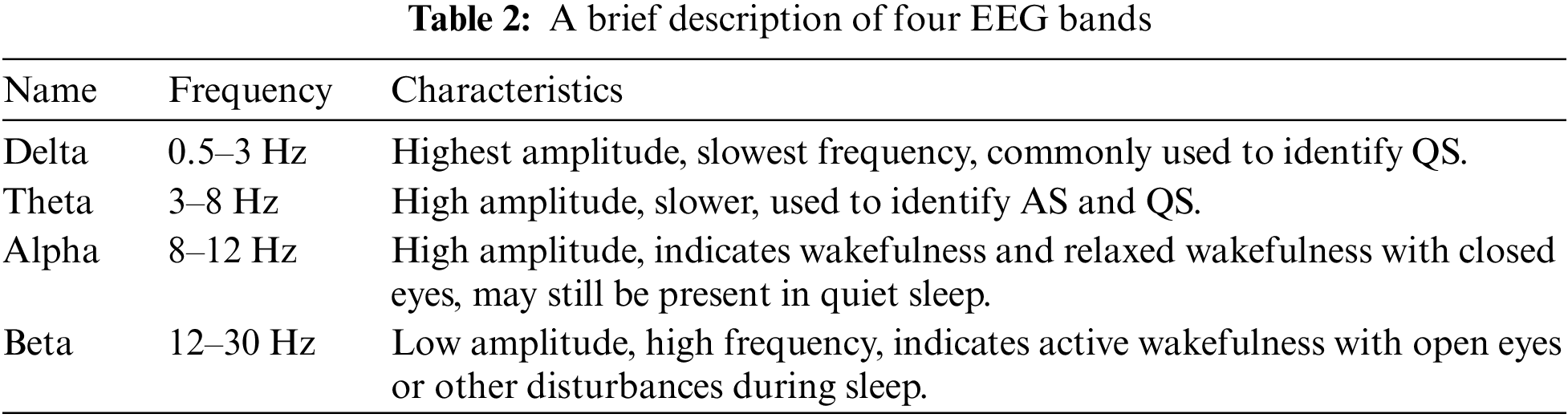
In this step, 8 time-domain and 4 frequency-domain attributes are extracted from each EEG signal. These 12 features are combined together to generate an input vector of size 108. Fast Fourier Transform (FFT) is utilized to extract the frequency domain features of the EEG channels. Then the mean frequencies are extracted from all bands, i.e., Delta (0.5–3 Hz), Theta (3–8 Hz), Alpha (8–12 Hz), and Beta (12–30 Hz). Table 2 provides a brief description of these four EEG bands. Each EEG channel’s time and frequency domain features are listed in Fig. 1.

3.5 Hyper-Parameter Tuning

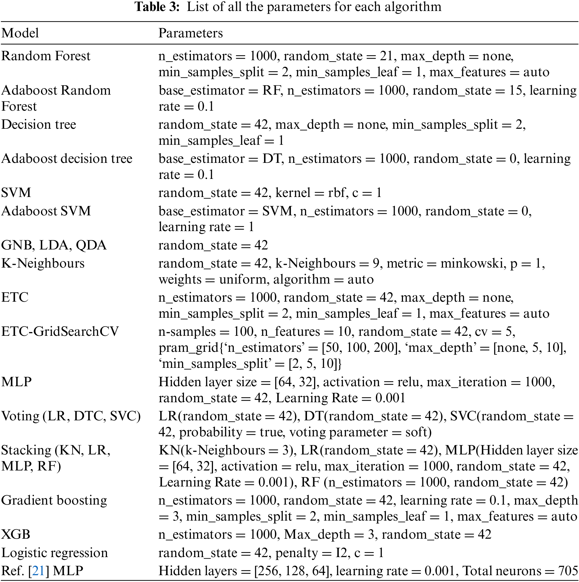
To use a machine learning model for different problems, hyperparameter optimization is required [39]. Choosing the best hyper-parameters will always improve the performance of a model. Many automatic optimization techniques are available, such as AutoML hyper-parameter tuning, RandomizedSearchCV, and GridSearchCV. While RandomizedSearchCV and GridSearchCV require users to specify a range of parameters for testing, autoML hyper-parameter tuning is time-saving and automatically selects the most appropriate values. Through the use of grid search or Bayesian optimization strategies, AutoML tunes hyperparameters, selects search strategies, and evaluates multiple models using performance metrics. A dynamic search space is updated based on results, a criterion is applied to terminate the search, and the best configuration is selected for the best performance of the model. By automating these processes, one can reduce manual effort, improve configurations, and enhance the performance of machine learning models. Therefore, autoML hyper parameter tuning is used. In this study, the AutoMLSearch class from the EvalML library was used to tune hyperparameters. As part of the analysis, the whole data was split into testing and training. AutoMLSearch was initialized with training data, a hyperparameter search was conducted, the best pipeline was selected based on performance, the pipeline was evaluated on the test set, and the results were stored. As a result of this automated process, hyperparameters were explored efficiently and optimal configurations were identified for each algorithm. Each of the 18 algorithms used in this study and MLP employed in [21] has its own set of parameters, which are listed in Table 3. n_estimators represent the number of trees in the forest, whereas random_state controls the randomness in the machine learning model and it can only take positive integral values, but not negative integral values.

3.6 Random Forest

Random Forest is a powerful learning algorithm. This algorithm is applied as an ensemble technique, due to the fact that it makes the final decision based on the results of all the decision trees combined [40]. Besides being flexible and easy to use, it can be used for both classification and regression [41]. Due to the fact that Random Forest takes the average of all predicted results and cancels partiality, there is no overfitting problem. In addition, it handles missing values. In order to select the most contributing features for classification, it will provide relative feature importance. The feature importance in each decision tree is calculated as [42]:

fic=∑nic∑ni(1)

where, fic is feature importance for the column in the particular decision tree, nic is the node impurity of the particular column, and ni total node impurity in the whole decision tree. Node impurity measures how well a tree splits the data. In this case, the nic is:

nic=(nic,left)(nleft)+(nic,right)(nright)ni(2)

where nleft is the number of samples in the left child nodes and nright is the number of samples in the right child nodes [43]. As a result, the ni can be calculated as follows:

ni=∑c∈Cnic(3)

At node i, C represents the columns that are being split. Now, the value of fic from Eq. (1) can be normalized between 0 and 1 by dividing it by the sum of all feature importance values.

normfic=fic∑fic(4)

Now, the final importance of features from all Random Forest trees can be obtained by dividing the normalized feature importance value by the total number of trees in the designed Random Forest model.

RFfic=∑normficT(5)

where T is the total number of trees. So, the more trees a Random Forest has, the stronger a forest is. Random Forest will first select some random samples from the dataset provided, then construct a decision tree for each sample. After each decision tree has been evaluated, it will give predicted results. At the end, it will select the results with the most votes to make a final prediction. Fig. 3 illustrates the general working mechanism of the Random Forest classifier on a data set. By setting random_state to 21 and using 1000 n_estimators in this particular research, an AutoMl-based Random Forest estimator is applied to EEG data. Its accuracy and kappa are 84.78% and 69.63%, respectively, which are the maximum accuracy and kappa for the categorization of sleep-wake stages.

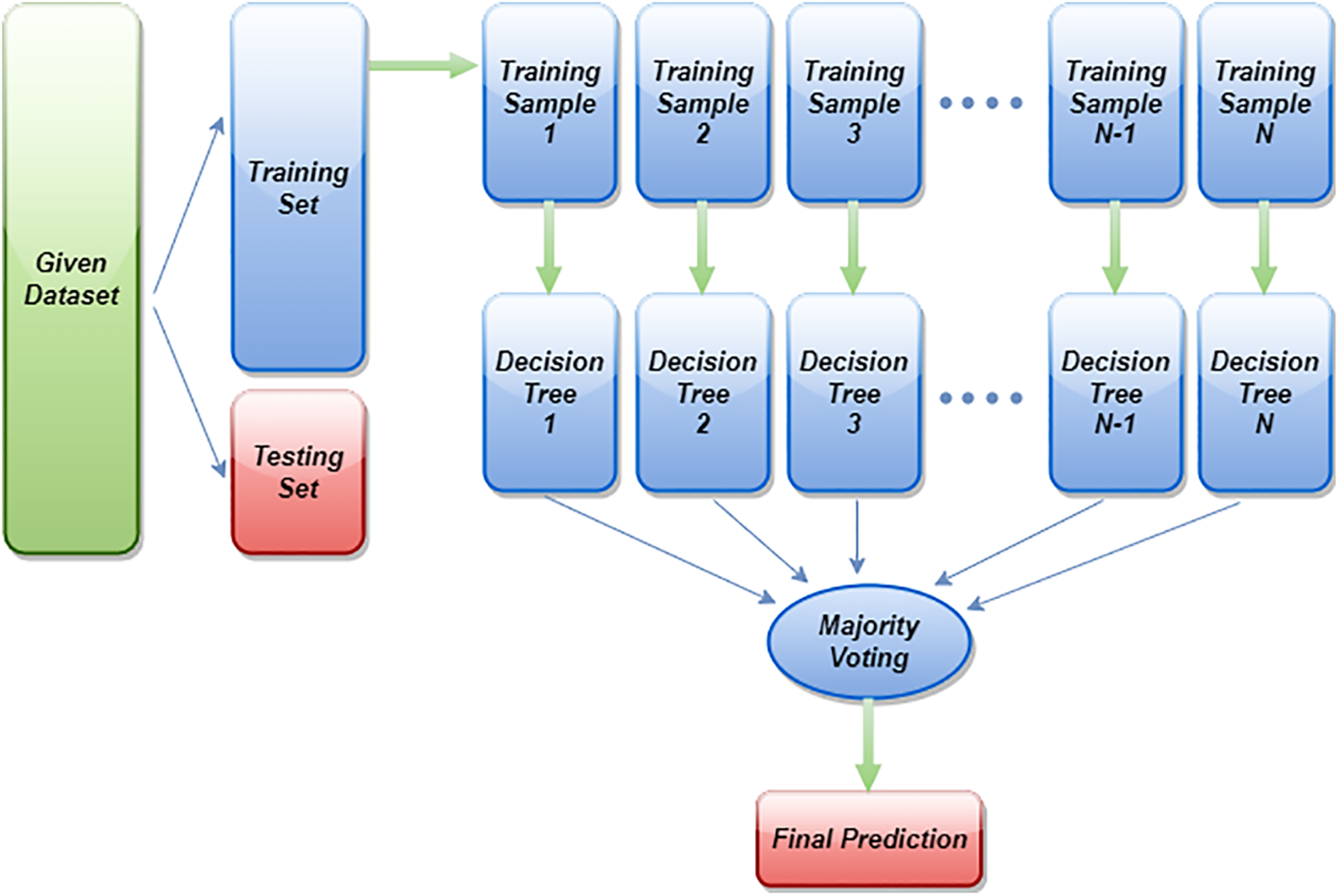
Figure 3: General diagram of Random Forest classifier implementation on a dataset

3.7 Adaboost Algorithm

Adaboost trains and deploys a set of trees in series, that is why called the ensemble method. It works on boosting principles, in which data samples that were misclassified by a previous weak classifier are reclassified by the new weak classifier. All the weak classifiers are connected in series to produce a strong classifier at the end. Basically, Adaboost combines a number of decision trees in the boosting process. These decision trees are called stumps. When the first decision tree/model is trained and deployed, the record which is falsely classified over the first model will be given more priority [44]. Only these records will be sent as input to the second model. Now the second tree will be trained in such a way that it will strictly observe the weaknesses in the previous tree. Now the weights of the previously miss-classified samples will be boosted in such a way that the next tree keeps the focus on correctly classifying the previously miss-classified data samples. The process will continue until a strong classifier is generated. One can increase the classification accuracy by adding in series the weak classifiers. However, this may result in severe overfitting [45]. Fig. 4 illustrates the general working mechanism of the Adaboost classifier on a data set of two classes and two features. As one can see from Fig. 4, that weak learner 2 enhances the results of weak learner 1 and results in a strong learner that has the decision boundaries of both learners. The Adaboost algorithm works by assigning some weights to the data points [44].

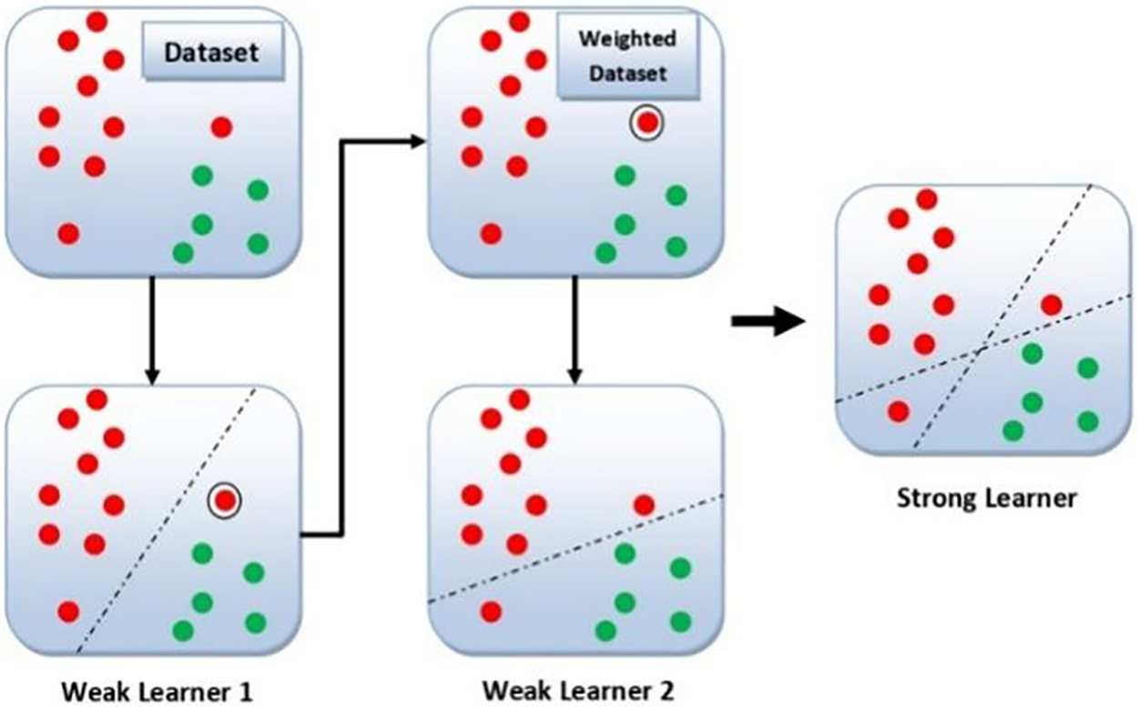
Figure 4: General diagram of Adaboost classifier

W(xn,yn)=1N(6)

where N represents the total number of data points and n=1,2,3,…,N. The next step is to determine which stump classifies the data in a good way. The tree with the lowest Gini index must be selected [40]. After that, the stump’s performance and total error must be calculated as follows [40]:

Performance=12×loge⁡1−TotalErrorTotalError(7)

The total error must be between 0 and 1, where 1 represents a horrible stump and 0 shows a perfect stump, respectively. Now, to calculate the updated weights of data points, the following formula could be used [40]:

Newweight=Oldweight×e(Performance)(8)

If the data is correctly classified, the value of performance will be negative otherwise it will be positive. Now, the weights must be updated and normalized accordingly. All these steps must be repeated until a low training error is obtained. So, an autoML-based Adaboost Random Forest estimator is applied to EEG data by setting the value of random_state as 15 and using 1000 n_estimators. As a base_estimator, a Random Forest classifier with 2000 n_estimators was used. For the categorization of sleep-wake stages, its accuracy and kappa came out as 84.59% and 69.24%, respectively. Since this research was designed to achieve accurate classification of neonatal sleep and wake using EEG data, the emphasis was placed on Random Forest and Adaboost Random Forest due to their outclass performance in terms of accuracy and all other performance parameters. However, a brief explanation of all other 16 algorithms is given below.

Decision Tree: A decision tree is made up of nodes representing features, branches representing rules, and leaves representing the outcome. The purpose of decision trees is to optimize the information gained or minimize impurities by recursively splitting the data according to the most advantageous feature. The classification is based on a single decision tree in this combination. Adaboost DT: In Adaboost DT, DT is used as a base estimator. As each tree is trained, its mistakes are corrected, producing a sequence of decision trees. Final predictions are based on aggregating all prediction trees, with more accurate trees being given a higher weight. SVM: This classifying algorithm divides features into classes by determining an optimized hyperplane. It aims to minimize classification errors while maximizing the margin between classes. Data is mapped into higher-dimensional spaces by kernel functions, so that linear separations can be achieved. Adaboost SVM: Adaboost SVM uses SVM as a base estimator. The next SVM corrects the mistakes of the previous SVM as it creates a sequence of SVMs. SVMs are combined into a final prediction, with more accurate SVMs given greater weight. GNB: Naive Bayes is a classification algorithm based on Bayes’ theorem, which assumes features are independent. In GNB, continuous features are assumed to follow a Gaussian distribution. Given the observed features, the class conditional probability is calculated and predictions are based on the likelihood of each class achieving that outcome. QDA: QDA uses quadratic decision boundaries as its basis for classifying data. For each class, a quadratic function is used to estimate the class-conditional probability densities. By calculating posterior probabilities, QDA predicts which class will have the highest probability given the observed features. LDA: LDA assumes that each class has a Gaussian distribution. Probability densities and prior probabilities are estimated for each class condition. Using LDA, the most probable class under each set of features is determined based on the posterior probability of the class given those features. KN: In KN, the k nearest training samples are taken into account when making predictions from a feature space. Majority voting among the k nearest neighbors determines the label for the class. ETC: Similar to Random Forest, Extra Trees are also ensemble learning methods. By creating multiple splits using random numbers, multiple decision trees are built, and the split with the lowest number of impurities is selected. A majority vote or an average of all predictions makes the final prediction. ETC with GridSearchCV: ETC with GridSearchCV optimizes hyperparameters and improves performance of ETC. MLP: MLP neural networks transform inputs into desired outputs through a series of non-linear transformations, identifying optimal weights and biases along the way. To minimize the error between predicted and actual outputs, backpropagation is used to adjust the weights and biases during training. Voting Classifier: The proposed Voting Classifier combines the predictions of multiple classifiers, including LR, DT, and SVC, using a voting strategy (e.g., majority voting or weighted voting). The final prediction is made based on the combined decisions of all classifiers. Stacking Classifier: The proposed stacking classifier utilizes multiple classifiers, including KN, LRR, MLP, and Random Forest, using a meta-classifier. Predicting the final outcome of a classifier is done through input features which were derived from the base classifiers. These classifiers were trained on training data prior to the metaclassifier was created. GB: Gradient boosting integrates multiple weak learners (e.g., decision trees) in a stepwise fashion. In this method, weak learners are trained to correct the previous learner’s mistakes. In order to get the final prediction, the predictions of all the weak learners are combined, and the predictions of the most accurate learners are given a higher weight. XGB: XGB, or XGBoost, is a gradient boosting method optimized for large datasets. Through a regularized model, the algorithm reduces overfitting and uses a more efficient tree construction algorithm, improving upon traditional gradient boosting. LR: In LR, features are mapped to a probability of belonging to a class based on a linear classification algorithm. A logistic function is used to convert the linear output into probabilities after estimating the coefficients of the linear equation using maximum likelihood estimation. The list of parameters for all algorithms used in this study is already presented in Table 3.

4  Results

The proposed scheme is tested and evaluated via different performance matrices such as confusion matrix, accuracy, Cohen’s kappa, recall, precision, Mathew’s correlation coefficient, F1-score, specificity, sensitivity, ROC (Receiver Operating Characteristic) curve and precision-recall curve. Mathematically, these values of accuracy [42], Cohen’s kappa [46], recall [47], precision [47], Mathew’s correlation coefficient [46], F1-score [44], sensitivity [28,45], and specificity [28,45] are computed as follows:

Acc=(TP+TN)(TP+TN+FP+FN)(9)

Kappa=2(TP.TN−FP.FN)(TP+FP).(FP+TN)+(TP+FN).(FN+TN)(10)

Rec=TP(TP+FN)(11)

Pre=TP(TP+FP)(12)

MCC=(TP.TN−FP.FN)(TP+FP)(TP+FN)(TN+FP)(TN+FN)(13)

F1−sco=2×Pre×RecPre+Rec(14)

Sen=TP(TP+FN)(15)

Spe=TN(TN+FP)(16)

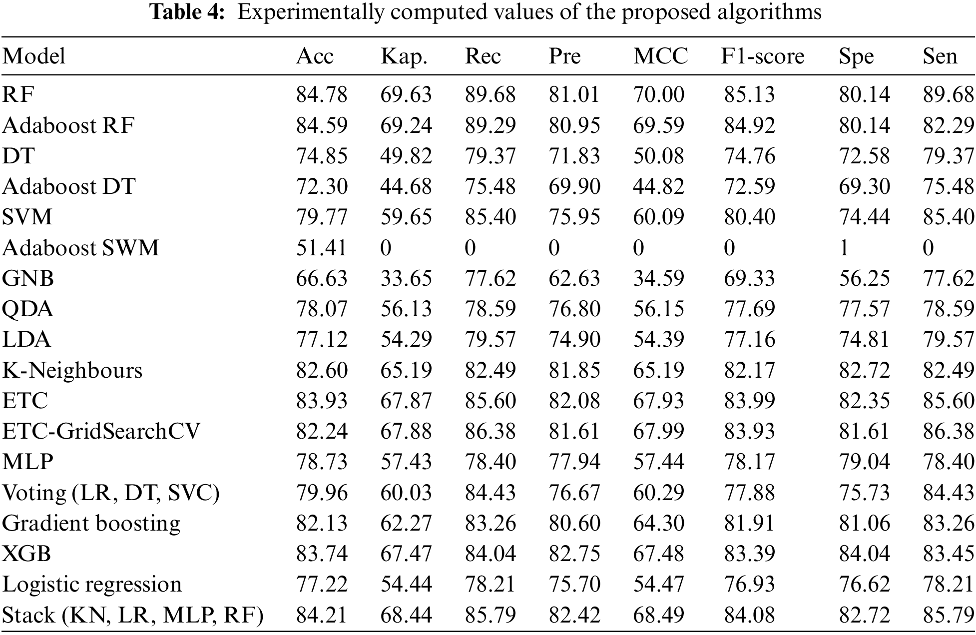
The experimentally computed values of all the above-mentioned performance matrices for all the proposed algorithms are shown in Table 4.

4.1 Confusion Matrix

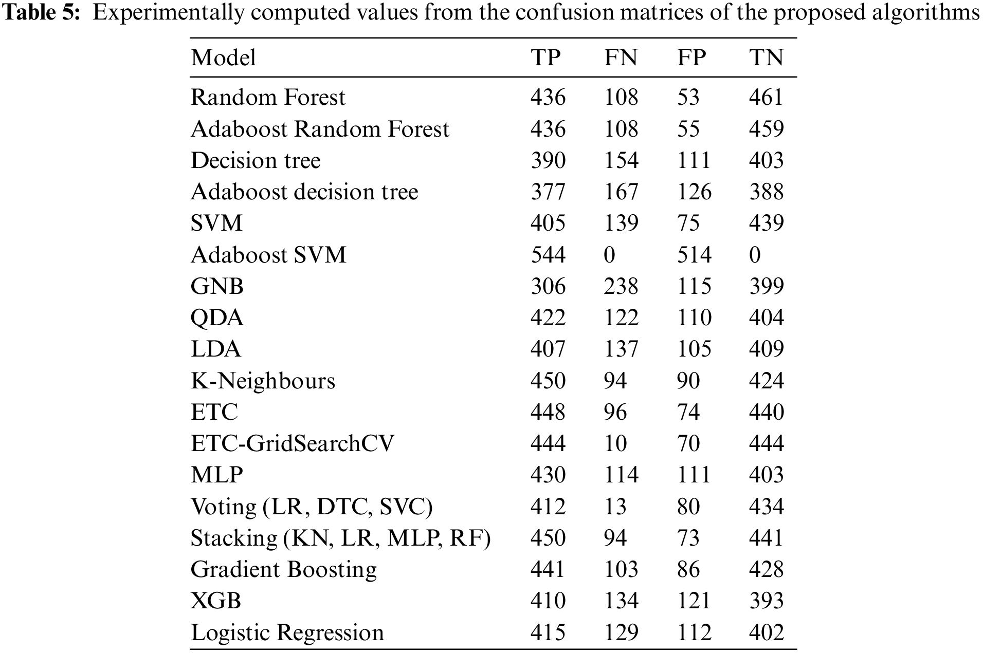
Classification models are evaluated using a confusion matrix. This matrix shows predictive and actual classification information. The binary class confusion matrix is shown in Fig. 5a. In Fig. 5a, TP represents true positives (sleep predicted as sleep), TN represents true negatives (wake predicted as wake), FP represents false positives (sleep predicted as wake), and FN represents false negatives (wake predicted as sleep). Confusion matrix for AutoML-based Random Forest classifier is illustrated in Fig. 5b. Table 5 shows the values of TP, FN, FP, and TN from the confusion matrices of all applied models.

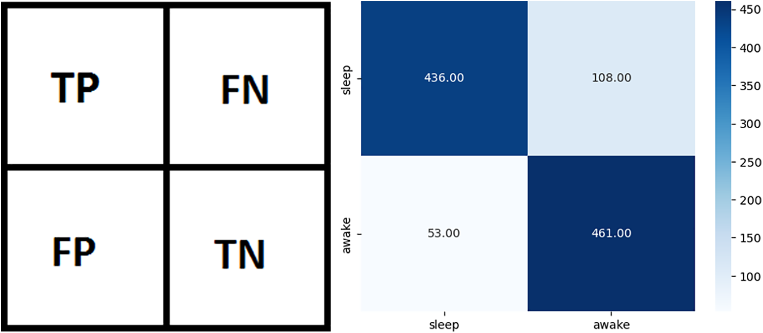
Figure 5: Confusion matrices (a) General binary classification confusion matrix, (b) Confusion matrix for AutoML-based Random Forest classifier

4.2 ROC Curve

A ROC curve shows a model’s performance at every classification threshold. In the ROC curve, two parameters are plotted: TPR (True Positive Rate) and FPR (False Positive Rate). Where TPR is same as recall and it is already defined in Eq. (11) and FPR is defined as:

FPR=FP(FP+TN)(17)

The closer the ROC curve is to the top left corner, the better the model is at categorizing the data. In ROC graphs, AUC is the Area Under the Curve, with values ranging from 0 to 1. Excellent models have AUC near 1, which indicates good separation capability. Models with an AUC near 0 have the lowest degree of separation, so their AUC is the lowest. An AUC of 0.5 means a model is unable to separate classes at all. Fig. 6a shows a ROC curve for an AutoML-based Random Forest classifier.

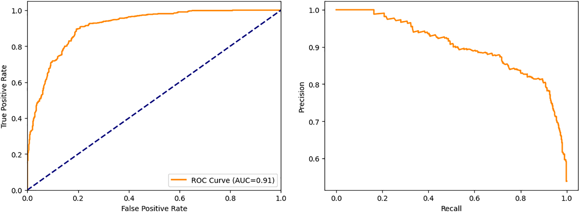
Figure 6: Performance curves (a) ROC curve for autoML-based random forest classifier, (b) Precision-recall curve for AutoML-based Random Forest classifier

4.3 Precision-Recall Curve

For different thresholds, the precision-recall curve shows how precision varies with recall. Classifiers with high precision and recall have a large area under the curve and always hug the upper right corner of the graph. Fig. 6b shows a precision-recall curve for an AutoML-based Random Forest classifier.

In general, ROC curves and precision-recall curves deal with class imbalance in different ways. Precision-recall curves are insensitive to class imbalance and measure how well a classifier accurately predicts a positive class. While ROC curves are sensitive to class imbalance and measure how well a classifier distinguishes between two classes. In addition, the ROC curve allows threshold selection that balances the false positive and true positive rate trade-offs. In Fig. 7, the ROC and Precision-recall curves for all the classifiers are compared.

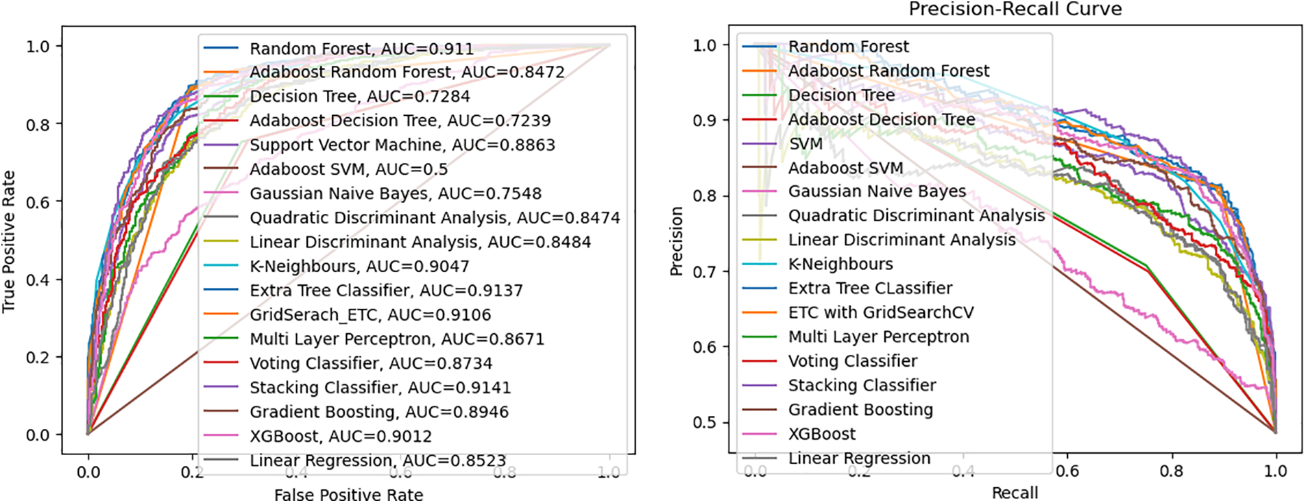
Figure 7: Performance curves (a) A comparison of the ROC curves for all classifiers, (b) A comparison of the precision-recall curves for all classifiers

5  Discussions

There are several algorithms for EEG-based automatic neonatal sleep staging, but most researchers have not defined wake as a distinct state. In most cases, wake and AS I combined to form an LVI stage. This causes the two sleep stages to be intermixed. Previously, a multilayer perceptron neural network was designed for the classification of sleep and wake as distinct states, achieving an accuracy of 82.53% [21]. This study aimed to improve accuracy and kappa of [21] by using the same dataset and proposing 18 different classification models. Firstly, EEG recordings were obtained from 19 infants in the NICU at a CHFU, China. The data is obtained from neonates with post-menstrual age 37 ± 05 weeks. Firstly, in the EEG-lab, a FIR filter was used to filter recordings with frequencies between 0.3 and 35 Hz. After filtering, the multi-channel EEG signals were segmented into 30 s epochs and each epoch was assigned a label. Finally, artifacts are removed based on annotations by doctors (PR and SR). Thus, after pre-processing, 3535 segments are left for testing and training. A total of 12 features were extracted, of which 8 were in the time domain and 4 in the frequency domain. An input vector of size 108 will be created by combining the 12 features from each of the 9 EEG channels. The most significant features were in the frequency domain. Four frequency bands (delta, theta, alpha, and beta) were extracted using FFT, and mean amplitudes of each band were determined. Feature scaling was applied after feature extraction. After feature scaling, an automatic optimization technique such as AutoML hyperparameter tuning is used to improve the performance of models. As an input, all autoML-based classifiers take a vector of size 108 consisting of the joint attributes of nine channels. 30% of the total EEG data is used for testing these classifiers and the remaining 70% is used for training purposes. Moreover, every algorithm was trained and tested with the same data.

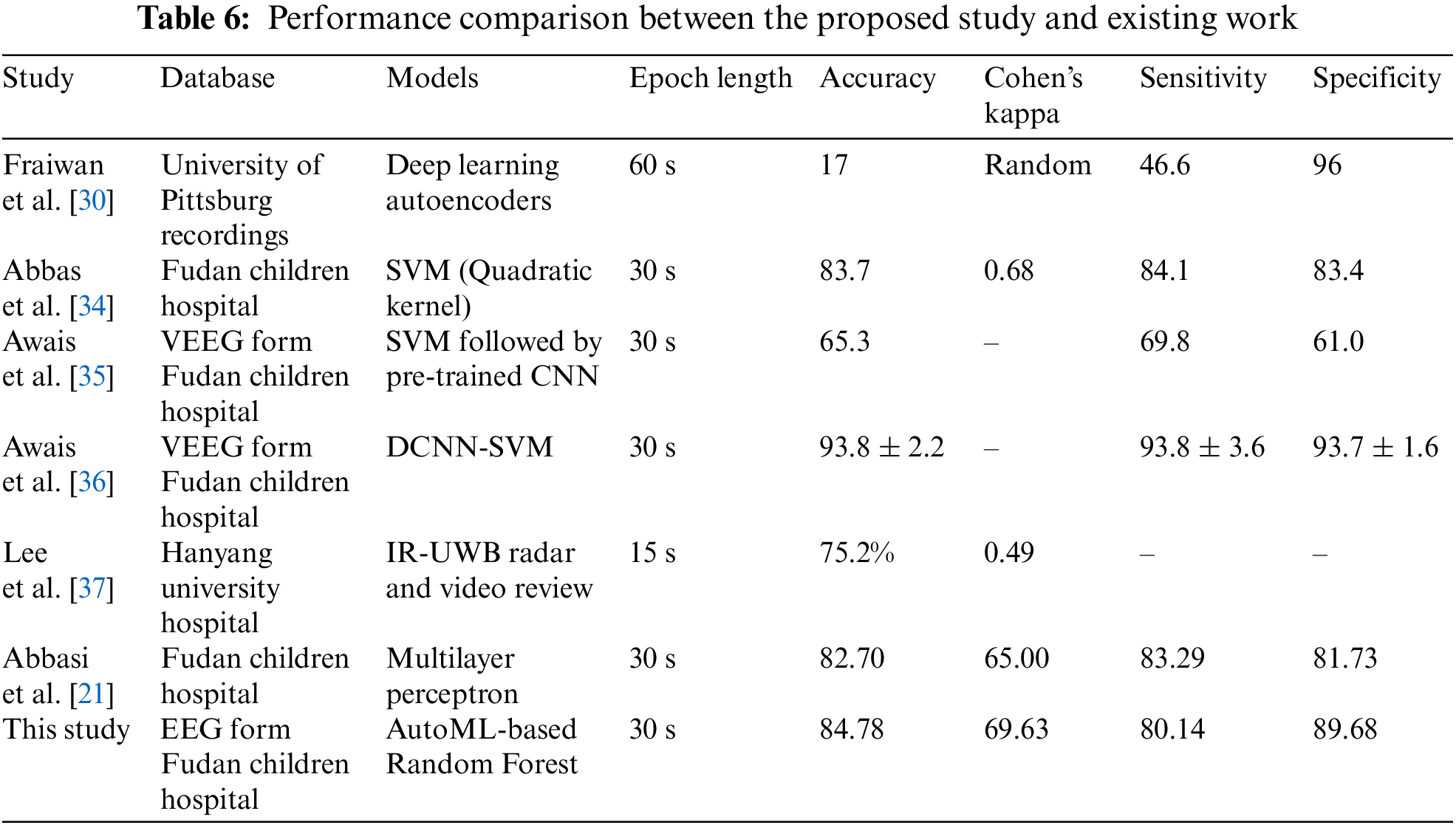
This study applied 18 different machine learning algorithms and tested their performance. Since this research was designed to achieve accurate classification of neonatal sleep and wake using EEG data, the emphasis was placed on Random Forest and Adaboost Random Forest due to their outclass performance in terms of accuracy and all other performance parameters. Each of the 18 algorithms used in this study and MLP employed in [21] has its own set of hyper-parameters, which are listed in Table 3. The experimentally calculated results are demonstrated in Table 4. These results are computed based on a binary class, i.e., sleep or wake. Thus, from Table 4, one can see that for the autoML-based Random Forest the accuracy and kappa are 84.78% and 69.63% respectively, which are the maximum accuracy and kappa for sleep-wake categorization. In addition, the accuracy and kappa values of the autoML-based Adaboost Random Forest and stacking classifier have also been improved. In the autoML-based Adaboost Random Forest model, accuracy and kappa were 84.59% and 69.24%, respectively; in the stacking classifier, accuracy and kappa were 84.21% and 68.44%. The accuracy and kappa for [21] was 82.7% and 65%, respectively. Confusion matrix for autoML-based Random Forest is illustrated in Fig. 5b. While for the other algorithms, the values of confusion matrices are listed in Table 5. It is clear from Table 5 that the computed values for TP and TN in the case of autoML-based Random Forest are very large as compared to all other applied algorithms. Moreover, Fig. 6a shows the ROC curve for an autoML-based Random Forest classifier. This model is better at categorizing data since the ROC curve is closer to the top left corner. It is also noteworthy that the AUC value of the model is 0.91, which indicates that it is capable of good separation. A plot of precision-recall is shown in Fig. 6b. Because the curve is closer to the right corner and the area under the curve is also high, it can be concluded that this classifier has high precision and recall, which makes it better at classification. The proposed autoML-based Random Forest classifier is also performing outclass in terms of recall, precision, MCC, F1-score, sensitivity, and specificity. The experimentally computed recall, precision, MCC, F1-score, sensitivity, and specificity values for autoML-based Random Forest are 89.68%, 81.01%, 70%, 85.13%, 80.14%, and 89.68%, respectively. Furthermore, for [21], the values of sleep F1-score, wake F1-score, sensitivity, and specificity are 81.45%, 82.55%, 83.29%, and 81.73%, respectively. Table 6 gives a Performance comparison between the proposed study and existing work on the same dataset. It can be seen from Table 6, that the authors in [36] achieved more accuracy because they used video EEG data not aEEG data. However, infant’s faces and voices can be found in EEG video data, raising privacy concerns. Thus, based on all the above discussion and proofs, the autoML-based Random Forest performed outclasses in terms of accuracy, kappa and other performance parameters and therefore, outclasses all other algorithms.

This study’s main limitation is that only 19 subjects were used, which is a very small sample size. The performance and effectiveness of the algorithm may be improved by using a larger dataset. Moreover, artifacts were manually removed at the prepossessing stage in this study. A future study can design a model that automatically removes these artifacts. This will enable the proposed method to be used practically in the NICU. It would also be possible to categorize more sleep stages, such as Active Sleep (AS), Quiet Sleep (QS), and Wake. Similarly, to enhance performance, more data can be utilized.

6  Conclusion

In this study, multi-channel EEG data and autoML-based 18 different estimators are utilized to classify neonate's sleep-wake states. Each of these estimators takes a vector of size 108 as input, containing the joint attributes of nine channels. For training and testing of the proposed approach, 3525 30-s segments of EEG recordings from 19 infants were used. The data is obtained from neonates at post-menstrual age 37 ± 05 weeks. Random Forest, Adaboost Random Forest, DT, Adaboost Decision Tree, SVM, Adaboost SVM, GNB, QDA, LDA, KNeighbours, Ensemble ETC, ETC with GridSearchCV, MLP, Voting Classifier (LR, DT Classifier, SVC), Stacking Classifier (KNeighbours, LR, MLP, Random Forest), GB, XGB, LR, and reference [21] were applied to the same dataset and their results are compared. Compared to the study in [21], which classified sleep and wake stages using MLP neural networks, this study achieved higher accuracy. A maximum accuracy of 84.78% and kappa of 69.63% is achieved for autoML-based Random Forest. The study shows that multi-channel EEG signals can be successfully classified by autoML-based approaches for neonatal sleep-wake classification and can help healthcare providers in the early identification and treatment of sleep-related issues in neonates.

7  Future Recommendations

In the future, the accuracy could be improved as well as the ability to classify further sleep states i.e., Active Sleep (AS), Quite Sleep (QS), and Wake. To enhance the performance of the proposed methodology, more data can be utilized. Moreover, in the prepossessing stage, the artifacts were manually removed, but in future, an automatic removal model can be designed to remove these artifacts.

Acknowledgement: Not applicable.

Funding Statement: This research work is funded by Chinese Government Scholarship. The findings and conclusions of this article are solely the responsibility of the authors and do not represent the official views of the Chinese Government Scholarship.

Author Contributions: Study conception and design: Hafza; data collection: Saadullah; analysis and interpretation of results: Hafza, Wei, Muhammad; draft manuscript preparation: Hafza, Saadullah. All authors reviewed the results and approved the final version of the manuscript.

Availability of Data and Materials: The dataset analyzed during the current study is not publicly available due to lack of permission from children’s hospital affiliated with Fudan University but codes are available from the corresponding author on reasonable request.

Ethics Approval: Authors would like to inform you that the neonate picture in Fig. 1 is the first author's own daughter. She has given her consent to use the picture for publication.

Conflicts of Interest: The authors declare that they have no conflicts of interest to report regarding the present study.

References

1. T. L. Baker, “Introduction to sleep and sleep disorders,” Medical Clinics of North America, vol. 69, no. 6, pp. 1123–1152, 1985. [Google Scholar] [PubMed]

2. L. Eliot, “ What’s going on in there,” in How the Brain and Mind Develop in the First Five Years of Life, vol. 294, no. 5, 1999. https://www.researchgate.net/publication/31862386 (accessed on 24/04/2023). [Google Scholar]

3. C. C. Thiedke, “Sleep disorders and sleep problems in childhood,” American Family Physician, vol. 63, no. 2, pp. 277, 2001. [Google Scholar] [PubMed]

4. M. El-Sheikh and A. Sadeh, “I. sleep and development: Introduction to the monograph,” Monographs of the Society for Research in Child Development, vol. 80, no. 1, pp. 1–14, 2015. [Google Scholar] [PubMed]

5. T. T. Dang-Vu, M. Desseilles, P. Peigneux and P. Maquet, “A role for sleep in brain plasticity,” Pediatric Rehabilitation, vol. 9, no. 2, pp. 98–118, 2006. [Google Scholar] [PubMed]

6. S. N. Graven and J. V. Browne, “Sleep and brain development: The critical role of sleep in fetal and early neonatal brain development,” Newborn and Infant Nursing Reviews, vol. 8, no. 4, pp. 173–179, 2008. [Google Scholar]

7. S. M. Ludington-Hoe, M. W. Johnson, K. Morgan, T. Lewis, J. Gutman et al., “Neurophysiologic assessment of neonatal sleep organization: Preliminary results of a randomized, controlled trial of skin contact with preterm infants,” Pediatrics, vol. 117, no. 5, pp. e909–e923, 2006. [Google Scholar] [PubMed]

8. M. H. Kohrman and P. R. Carney, “Sleep-related disorders in neurologic disease during childhood,” Pediatric Neurology, vol. 23, no. 2, pp. 107–113, 2000. [Google Scholar] [PubMed]

9. K. C. Voos, A. Terreros, P. Larimore, M. K. Leick-Rude and N. Park, “Implementing safe sleep practices in a neonatal intensive care unit,” The Journal of Maternal-Fetal & Neonatal Medicine, vol. 28, no. 14, pp. 1637–1640, 2015. [Google Scholar]

10. W. H. Spriggs, Essentials of Polysomnography: A Training Guide and Reference for Sleep Technicians. Burlington, MA, USA: Jones & Bartlett, 2014. [Google Scholar]

11. A. R. Hassan and M. I. H. Bhuiyan, “An automated method for sleep staging from EEG signals using normal inverse gaussian parameters and adaptive boosting,” Neurocomputing, vol. 219, pp. 76–87, 2017. [Google Scholar]

12. A. R. Hassan and M. I. H. Bhuiyan, “A decision support system for automatic sleep staging from EEG signals using tunable Q-factor wavelet transform and spectral features,” Journal of Neuroscience Methods, vol. 271, pp. 107–118, 2016. [Google Scholar] [PubMed]

13. S. Biswal, J. Kulas, H. Sun, B. Goparaju, M. B. Westover et al., “Sleepnet: Automated sleep staging system via deep learning,” arXiv preprint arXiv:1707.08262, 2017. [Google Scholar]

14. A. Dereymaeker, K. Pillay, J. Vervisch, S. Van Huffel, G. Naulaers et al., “An automated quiet sleep detection approach in preterm infants as a gateway to assess brain maturation,” International Journal of Neural Systems, vol. 27, no. 6, pp. 1750023, 2017. [Google Scholar] [PubMed]

15. N. Koolen, L. Oberdorfer, Z. Rona, V. Giordano, T. Werther et al., “Automated classification of neonatal sleep states using EGG,” Clinical Neurophysiology, vol. 128, no. 6, pp. 1100–1108, 2017. [Google Scholar] [PubMed]

16. K. Pillay, A. Dereymaeker, K. Jansen, G. Naulaers, S. Van Huffel et al., “Automated EEG sleep staging in the term-age baby using a generative modelling approach,” Journal of Neural Engineering, vol. 15, no. 3, pp. 036004, 2018. [Google Scholar] [PubMed]

17. L. Marcuse, M. Schneider, K. Mortati, K. Donnelly, V. Arnedo et al., “Quantitative analysis of the EEG posteriordominant rhythm in healthy adolescents,” Clinical Neurophysiology, vol. 119, no. 8, pp. 1778–1781, 2008. [Google Scholar] [PubMed]

18. A. H. Parmelee Jr, W. H. Wenner, Y. Akiyama, M. Schultz and E. Stern, “Sleep states in premature infants,” Developmental Medicine & Child Neurology, vol. 9, no. 1, pp. 70–77, 1967. [Google Scholar]

19. J. A. Hobson, “A manual of standardized terminology, techniques and criteria for scoring of states of sleep and wakefulness in newborn infants,” Electroencephalography and Clinical Neurophysiology, vol. 33, no. 6, pp. 614–615, 1972. [Google Scholar]

20. D. Y. Barbeau and M. D. Weiss, “Sleep disturbances in newborns,” Children, vol. 4, no. 10, pp. 90, 2017. [Google Scholar] [PubMed]

21. S. F. Abbasi, J. Ahmad, A. Tahir, M. Awais, C. Chen et al., “EEG-based neonatal sleep-wake classification using multilayer perceptron neural network,” IEEE Access, vol. 8, pp. 183025–183034, 2020. [Google Scholar]

22. A. L. Loomis, E. N. Harvey and G. A. Hobart, “Cerebral states during sleep, as studied by human brain potentials,” Journal of Experimental Psychology, vol. 21, no. 2, pp. 127, 1937. [Google Scholar]

23. T. Lajnef, S. Chaibi, P. Ruby, P. E. Aguera, J. B. Eichenlaub et al., “Learning machines and sleeping brains: Automatic sleep stage classification using decision-tree multi-class support vector machines,” Journal of Neuroscience Methods, vol. 250, pp. 94–105, 2015. [Google Scholar] [PubMed]

24. M. Xiao, H. Yan, J. Song, Y. Yang and X. Yang, “Sleep stages classification based on heart rate variability and random forest,” Biomedical Signal Processing and Control, vol. 8, no. 6, pp. 624–633, 2013. [Google Scholar]

25. P. Fonseca, N. Den Teuling, X. Long and R. M. Aarts, “Cardiorespiratory sleep stage detection using conditional random fields,” IEEE Journal of Biomedical and Health Informatics, vol. 21, no. 4, pp. 956–966, 2016. [Google Scholar] [PubMed]

26. S. Gudmundsson, T. P. Runarsson and S. Sigurdsson, “Automatic sleep staging using support vector machines with posterior probability estimates,” in IEEE Int. Conf. on Computational Intelligence for Modelling, Control and Automation and Int. Conf. on Intelligent Agents, Web Technologies and Internet Commerce (CIMCAIAWTIC’06), vol. 2, pp. 366–372, 2005. [Google Scholar]

27. J. Turnbull, K. Loparo, M. Johnson and M. Scher, “Automated detection of tracé alternant during sleep in healthy full-term neonates using discrete wavelet transform,” Clinical Neurophysiology, vol. 112, no. 10, pp. 1893–1900, 2001. [Google Scholar] [PubMed]

28. O. de Wel, M. Lavanga, A. C. Dorado, K. Jansen, A. Dereymaeker et al., “Complexity analysis of neonatal EEG using multiscale entropy: Applications in brain maturation and sleep stage classification,” Entropy, vol. 19, no. 10, pp. 516, 2017. [Google Scholar]

29. A. H. Ansari, O. de Wel, K. Pillay, A. Dereymaeker, K. Jansen et al., “A convolutional neural network outperforming state-of-the-art sleep staging algorithms for both preterm and term infants,” Journal of Neural Engineering, vol. 17, no. 1, pp. 016028, 2020. [Google Scholar] [PubMed]

30. L. Fraiwan and K. Lweesy, “Neonatal sleep state identification using deep learning autoencoders,” in IEEE 13th Int. Colloquium on Signal Processing & its Applications (CSPA), Penang, Malaysia, pp. 228–231, 2017. [Google Scholar]

31. A. H. Ansari, K. Pillay, A. Dereymaeker, K. Jansen, S. Van Huffel et al., “A deep shared multiscale inception network enables accurate neonatal quiet sleep detection with limited EEG channels,” IEEE Journal of Biomedical and Health Informatics, vol. 26, no. 3, pp. 1023–1033, 2021. [Google Scholar]

32. R. Yu, Z. Zhou, S. Wu, X. Gao and G. Bin, “MRASleepNet: A multi-resolution attention network for sleep stage classification using single-channel EEG,” Journal of Neural Engineering, vol. 19, no. 6, pp. 066025, 2022. [Google Scholar]

33. H. Zhu, Y. Xu, N. Shen, Y. Wu, L. Wang et al., “MS-HNN: Multi-scale hierarchical neural network with squeeze and excitation block for neonatal sleep staging using a single-channel EEG,” IEEE Transactions on Neural Systems and Rehabilitation Engineering, vol. 31, pp. 2195–2204, 2023. [Google Scholar] [PubMed]

34. A. Abbas, H. S. Sheikh, H. Ahmad and S. F. Abbasi, “An IoT and machine learning-based neonatal sleep stage classification,” Manuscript on ResearchGate. https://www.researchgate.net/publication/369761857_An_IoT_and_Machine_Learning-based_Neonatal_Sleep_Stage_Classification (accessed on 08/05/2023) [Google Scholar]

35. M. Awais, X. Long, B. Yin, C. Chen, S. Akbarzadeh et al., “Can pre-trained convolutional neural networks be directly used as a feature extractor for video-based neonatal sleep and wake classification?,” BMC Research Notes, vol. 13, no. 1, pp. 1–6, 2020. [Google Scholar]

36. M. Awais, X. Long, B. Yin, S. F. Abbasi, S. Akbarzadeh et al., “A hybrid DCNN-SVM model for classifying neonatal sleep and wake states based on facial expressions in video,” IEEE Journal of Biomedical and Health Informatics, vol. 25, no. 5, pp. 1441–1449, 2021. [Google Scholar] [PubMed]

37. W. H. Lee, S. H. Kim, J. Y. Na, Y. H. Lim, S. H. Cho et al., “Non-contact sleep/wake monitoring using impulse-radio ultrawideband radar in neonates,” Frontiers in Pediatrics, vol. 9, pp. 782623, 2021. [Google Scholar] [PubMed]

38. A. L. Satomaa, O. Saarenpää-Heikkilä, E. J. Paavonen and S. L. Himanen, “The adapted American Academy of Sleep Medicine sleep scoring criteria in one month old infants: A means to improve comparability?,” Clinical Neurophysiology, vol. 127, no. 2, pp. 1410–1418, 2016. [Google Scholar] [PubMed]

39. L. Yang and A. Shami, “On hyperparameter optimization of machine learning algorithms: Theory and practice,” Neurocomputing, vol. 415, pp. 295–316, 2020. [Google Scholar]

40. L. Breiman, “Random forests,” Machine Learning, vol. 45, no. 1, pp. 5–32, 2001. [Google Scholar]

41. A. Parmar, R. Katariya and V. Patel, “A review on random forest: An ensemble classifier,” in Int. Conf. on Intelligent Data Communication Technologies and Internet of Things, Coimbatore, India, vol. 26, pp. 758–763, 2018. [Google Scholar]

42. M. Pal, “Random forest classifier for remote sensing classification,” International Journal of Remote Sensing, vol. 26, no. 1, pp. 217–222, 2005. [Google Scholar]

43. Z. Wu and W. Chu, “Sampling strategy analysis of machine learning models for energy consumption prediction,” in IEEE 9th Int. Conf. on Smart Energy Grid Engineering (SEGE), Oshawa, ON, Canada, pp. 77–81, 2021. [Google Scholar]

44. R. E. Schapire, “Explaining adaboost,” In: N. Vapnik (Ed.Empirical Inference: Festschrift in Honor of Vladimir, pp. 37–52, Berlin: Springer Berlin Heidelberg, 2013. [Google Scholar]

45. S. Misra, H. Li and J. He, “Noninvasive fracture characterization based on the classification of sonic wave travel times,” in Machine Learning for Subsurface Characterization, vol. 4, Texas, USA: Gulf Professional Publishing, pp. 243–287, 2020. [Google Scholar]

46. D. Chicco, M. J. Warrens and G. Jurman, “The matthews correlation coefficient (MCC) is more informative than Cohen’s kappa and brier score in binary classification assessment,” IEEE Access, vol. 9, pp. 78368–78381, 2021. [Google Scholar]

47. S. Shaukat, A. Ali, A. Batool, F. Alqahtani, J. S. Khan et al., “Intrusion detection and attack classification leveraging machine learning technique,” in 14th Int. Conf. on Innovations in Information Technology (IIT), Al Ain, United Arab Emirates, pp. 198–202, 2020. [Google Scholar]