A Fusion of Residual Blocks and Stack Auto Encoder Features for Stomach Cancer Classification

1  Introduction

Gastrointestinal cancer, also known as digestive system cancer, refers to a group of cancers that occur in the digestive system or gastrointestinal tract, which includes the esophagus, stomach, small intestine, colon, rectum, liver, gallbladder, and pancreas [1,2]. These cancers develop when cells in the digestive system grow abnormally and uncontrollably, forming a tissue mass known as a tumor [3]. Depending on the type and stage of the disease, the symptoms of gastrointestinal cancer might include stomach discomfort, nausea, vomiting, changes in bowel habits, weight loss, and exhaustion [4]. According to the National Institute of Health, one out of twelve deaths related to cancer is due to gastrointestinal cancer. Moreover, each year more than one million new cases of gastrointestinal cancer are diagnosed. Gastrointestinal Tract cancer may be treated by surgery, chemotherapy, radiation therapy, or a combination. Detection and treatment at an early stage can enhance survival chances and minimize the risk of complications [5]. Despite a gradual decrease in gastric cancer incidence and mortality rates over the past 50 years, it remains the second most frequent cause of cancer-related deaths globally. However, from 2018 to 2020, both colorectal and stomach cancer have shown an upward trend in their rates [6]. Global Cancer Statistics show that 26.3 percent of total cancer cases are from gastrointestinal cancer, whereas the mortality rate is 35.4 percent among all cancers [7].

Identifying and categorizing gastrointestinal disorders subjectively is time-consuming and difficult, requiring much clinical knowledge and skill [8]. Yet, the development of effective computer-aided diagnosis (CAD) technologies that can identify and categorize numerous gastrointestinal disorders in a fully automated manner might reduce these diagnostic obstacles to a great extent [9]. Computer-aided diagnosis technologies can be of great value by aiding medical personnel in making accurate diagnoses and identifying appropriate therapies for serious medical diseases in their early stages [10,11]. Over the past few years, the performance of diagnostic-based artificial intelligence (AI) computer-aided diagnosis tools in various medical fields has been significantly improved with the use of deep learning algorithms, particularly artificial neural networks (ANNs) [12]. Generally, these ANNs are trained using optimization algorithms such as stochastic gradient descent [13] to achieve the best accurate representation of the training dataset.

DL, which refers to deep learning, is a statistical approach that enables computers to automatically detect features from raw inputs, such as structured information, images, text, and audio [14,15]. Many areas of clinical practice have been profoundly influenced by the significant advances made in AI based on DL [16,17]. Computer-aided diagnosis systems are frameworks that use computational-based help to detect any disease. CAD systems in gastroenterology increasingly use artificial intelligence (AI) to improve the identification and characterization of abnormalities during endoscopy [18]. The CNN, a neural network influenced by the visual cortex of life forms, uses convolutional layers with common two-dimensional weight sets. This enables the algorithm to recognize spatial data and employ layer clustering to filter out less significant information, eventually conveying the most pertinent and focused elements [19]. However, these classifiers face a challenge in interpretability because they are often seen as “black boxes” that deliver accurate outcomes without explaining them [20]. Despite technological developments, image classification for lesions of the gastrointestinal system remains difficult due to a lack of databases containing sufficient images to build models. In addition, the quality of accessible images has impeded the application of CNN models [21].

1.1 Major Challenges

In this work, Artificial Neural Networks (ANN) and Deep Neural Networks (DNN) extract the features of images from the Hyper-Kvasir dataset. The dataset contains twenty-three gastrointestinal tract classes with images in each class. However, some classes have only a few images, creating a data misbalancing problem. Data augmentation techniques are used for classes with fewer images to address this issue. Furthermore, feature selection techniques are implied to obtain the best features among feature sets.

1.2 Major Contributions

The major contributions of the proposed method are described as follows:

–   Proposed fusion-based contrast enhancement technique based on the mathematical formulation of local and global information-enhanced filters, called Duo-contrast.

–   A new CNN architecture is designed based on the concept of pretrained Nasnetmobile. Several residual blocks have been added to increase the learning capability and reduction of parameters.

–   A stack Auto Encoder-Decoder network is designed that consists of five convolutional layers in the encoder phase and five in the decoder phase.

–   The extracted features have been optimized using improved Marine Predator optimization and Slime Mould optimization algorithm.

–   A new parallel fusion technique is proposed to combine the important information of both deep learning models.

–   A detailed experimental process in terms of accuracy, confusion matrix, and t-test-based analysis has been conducted to show the significance of the proposed framework.

The rest of the manuscript is structured as follows: Section 2 describes the significant related work relevant to the study. Section 3 outlines the methodology utilized in the research, including the tools, methods, and resources employed. Section 4 comprises a discussion of the findings acquired from the study. Section 5 provides the conclusions of the research.

2  Related Work

Gastrointestinal tract classification is a hot topic in research. In recent years, researchers have achieved important milestones in this work domain [22]. In their article, Borgli et al. introduced the Hyper-Kvasir dataset, which contains millions of images of gastrointestinal endoscopy examinations from Baerum Hospital located in Norway. The labeled images in this dataset can be used to train neural networks for discrimination purposes. The authors conducted experiments to train and evaluate classification models using two commonly used families of neural networks, ResNet and DenseNet, for the image classification problem. The labeled data in the Hyper-Kvasir dataset consist of twenty-three classes of gastrointestinal disorders. While the authors achieved the best results by combining ResNet-152 and DenseNet-161, the overall performance was still unsatisfactory due to imbalanced development sets [23]. In their proposal, Igarashi et al. employed AlexNet architecture to classify more than 85,000 input images from Hirosaki University Hospital.

Moreover, the input images were categorized into 14 groups based on pattern classification of significant anatomical organs with manual classification. To train the model, the researchers used 49,174 images from patients with gastric cancer who had undergone upper gastrointestinal tract endoscopy. In comparison, the remaining 36,000 images were employed to test the model’s performance. The outcome indicated an impressive overall accuracy of 96.5%, suggesting its potential usefulness in routine endoscopy image classification [24]. Gómez-Zuleta [25] developed a deep learning (DL) methodology to detect polyps in colonoscopy procedures automatically. For this task, three models were used, namely Inception-v3, ResNet-50, and VGG-16. Knowledge transfer through transfer learning was adopted for classification, and the resultant weights were used to commence a fresh training process utilizing the fine-tuning technique on colonoscopy images. The training data consisted of a combined dataset of five databases comprising more than 23000 images with polyps and more than 47000 images without polyps for validation, respectively. The data was split into a 70 by 30 ratio for training and testing purposes. Different metrics such as accuracy, F1 score, and receiver operating characteristic curve, commonly known as ROC, were employed to evaluate the performance. Pertrained models such as Inceptionv3, VGG16, and Resnet50 models achieved accuracy rates of 81%, 73%, and 77%, respectively. The authors described that pretrained network models demonstrated an effective generalization ability towards the high irregularity of endoscopy videos, and their methodology may potentially serve as a valuable tool in the future [25]. The authors employed three networks to classify medical images from the Kvasir database. They began using a preprocessing step to eliminate noise and improve image quality. Then, they utilized data augmentation methods to progress the network’s training and a dropout method to prevent overfitting. Yet, the researchers acknowledged that this technique resulted in a doubling of the training time. The researchers also implemented Adam to optimize the loss to minimize error. Moreover, transfer learning and fine-tuning techniques are implied. The resulting models were then used to categorize 5,000 images into five distinct categories, with eighty percent of the database allocated for training and twenty percent for validation. The accuracy rates achieved by the models were 96.7% for GoogLeNet, 95% for ResNet-50%, and 97% for AlexNet [26].

The Kvasir-Capsule dataset, presented in [27], includes 117 videos captured using video capsule endoscopy (VCE). The dataset comprises fourteen different categories of images and a total of more than 47000 identified categorized images. VCE technology involves a small capsule with a camera, battery, and other components. To validate the labeled dataset, two convolutional neural networks (CNNs), namely, DenseNet_161 and ResNet_152, were used for training. The study utilized a cross-validation technique with definite cross-entropy-based loss to validate the models. They implemented this technique without class and with class weights and used weight-based sampling to balance the dataset by removing or adding images for every class. After evaluating the models, the best results were obtained by averaging the outcomes of both CNNs. The resulting accuracy rates were 73.66% for the micro average and 29.94% for the macro average.

Overall, the researchers improved their categorization of the Hyper-Kvasir dataset. Yet, a significant gap in the subject matter must be filled. So, it must utilize a wonderful hybrid strategy incorporating deep learning and machine learning methodologies to get exceptional outcomes. Using machine learning approaches to discover key characteristics and automated deep feature extraction to uncover them may help increase classification accuracy.

3  Proposed Methodology

The dataset used in this manuscript is highly imbalanced as some classes have few images. To resolve this problem, data augmentation techniques are adopted. Nasnetmobile and Stacked Autoencoders are used as feature extractors. Furthermore, the extracted feature vectors eV1 from Nasnetmobile and eV2 from Stacked Auto-encoder are reduced by applying feature optimization techniques. eV1 is fed to the Marine Predator Algorithm (MPA) [28] while eV2 is given as input to the Slime Mould Algorithm (SMA) [29] to extract selected feature vectors S (eV1) and S (eV2), respectively. Selected feature vectors S (eV1) and S (eV2) are fused. Moreover, artificial neural networks are used as classifiers to achieve results. Fig. 1 shows the proposed methodology used in this paper.

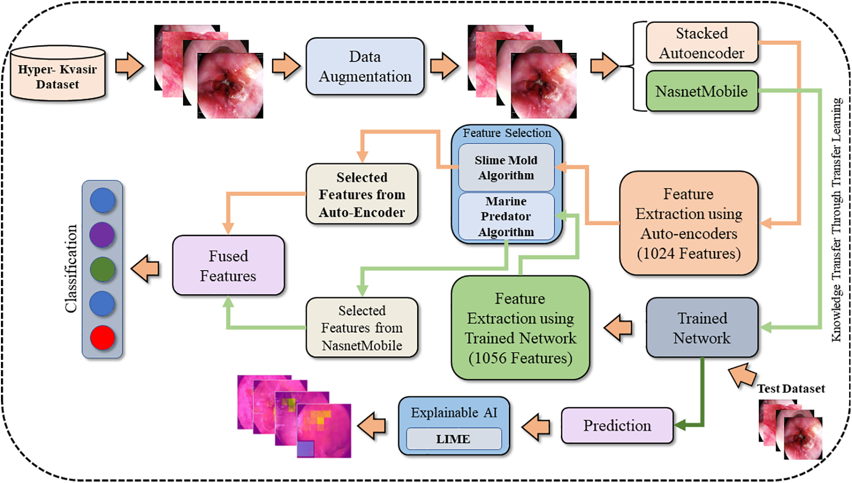
Figure 1: Proposed methodology of stomach cancer classification and polyp detection

3.1 Dataset Description

The Hyper-Kvasir dataset used in this study is a public dataset collected from Baerum Hospital in Norway [23]. The dataset contains 10,662 gastrointestinal endoscopy images categorized into 23 classes. Among twenty-three classes, sixteen belong to the lower gastrointestinal area, while seven are related to the upper gastrointestinal segment. Table 1 describes the data misbalancing problem, as some of the classes have very few numbers of images. To nullify the issue, data augmentation techniques are applied. Fig. 2 shows the sample images for each class.

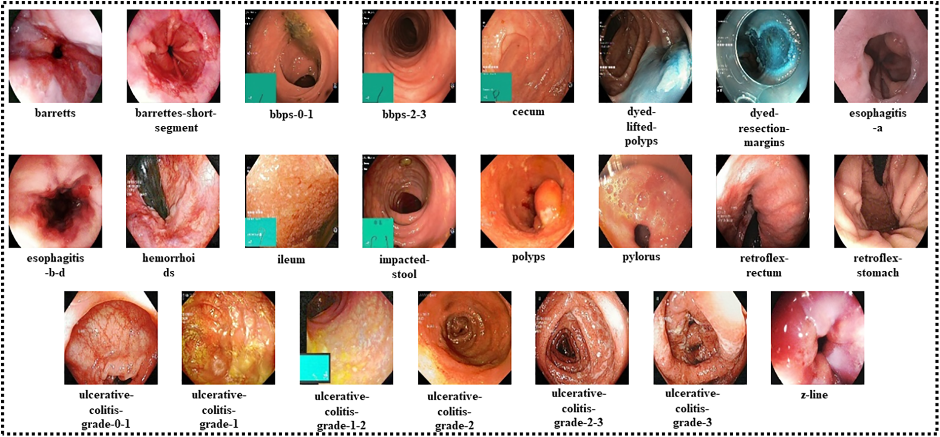
Figure 2: Sample images of each class of the Hyper-Kvasir dataset

3.2 Proposed Contrast Enhancement

Data is augmented by applying different image enhancement techniques on the whole Hyper-Kvasir dataset, as these techniques change spatial properties but do not affect the image orientation. Brightness Preserving Histogram Equalization (BPHE) [30] and Dualistic Histogram Equalization (DHE) [31] are used in preprocessing.

BPHE is a method employed in image processing to enhance an image’s visual quality by improving its contrast. This approach involves adjusting the distribution of intensity levels to generate a more uniform histogram. Unlike conventional histogram equalization techniques, brightness-preserving histogram equalization considers both bright and dark regions in an image. It independently adjusts the histograms of each region to retain the details in both bright and dark areas while enhancing the overall contrast. This technique is particularly useful in applications such as medical imaging, where preserving the details in both bright and dark regions is crucial. The input image is divided into two subparts; the first consists of pixels with low contrast values, while the second consists of pixels with high contrast values. Mathematically it is denoted as:

MInp=(Mlower)∪(Mhigher)(1)

Here,

(Mlower)={M(j,k)|M(j,k)≤Mmean,∀ M(j,k)∈M(2)

and

(Mhigher)={M(j,k)|M(j,k)≤Mmean,∀ M(j,k)∈M(3)

Moreover, a function of probabilistic density for both subparts is derived as:

(Densprob)l(Mt)=OltOl, Where t=0,1,2,…,N(4)

and

(Densprob)h(Mt)=OhtOh, Where t=N+1,N+2,…,N−K(5)

where Olt and Oht are the number of Mp in (Mlower) and (Mhigher), respectively. Moreover, the cumulative density functions for subparts are derived as:

Funcdl(Mt)=∑k=0t(Densprob)l(Mk)(6)

and

Funcdh(Mt)=∑k=N+1p(Densprob)h(Mk)(7)

The transform function for subparts is as follows:

TrfL(Mt)=M0(MN−M0)Funcdl(Mt)(8)

and

Trfh(Mt)=M0(MN−M0)Funcdh(Mt)(9)

The final image having an equalized histogram with preserved brightness can be obtained by combining both equations, that is:

ImgBPHE=TrfL(Mt) ∪ Trfh(Mt)(10)

In the above equation, ImgBPHE is the Brightness Preserved Histogram Equalized image.

DSIHE is an image enhancement approach that increases an image’s contrast by separating it into two subimages depending on a threshold value and then applying histogram equalization independently to each subimage. The significance of DSIHE resides in its capacity to improve the contrast of images containing dark and light areas. Contrast enhancement is done worldwide using classical histogram equalization, which can result in over enhancing bright parts and under enhancement of dark regions in an image. DSIHE tackles this issue by separating the picture into two subimages based on a threshold value that distinguishes between the light and dark regions. Afterward, histogram equalization is applied separately to each subimage, which helps to achieve an equilibrium across the two regions’ contrast enhancement. It has been demonstrated that the DSIHE technique enhances the aesthetic quality of medical images. It is an easy, computationally efficient, and straightforward strategy to implement in image processing systems.

Let MInp is an input image that is given to apply DSIHE, and the grey level of that image is MInp=Mgrey. Sub-images are denoted by MS1 and MS2. The center pixel index is denoted by Cpx.

MInp=MS1∪MS2(11)

MS1={MInp(i.j)|MInp(i.j)<Mgrey,∀MInp(i.j)∈MInp}(12)

MS2={MInp(i.j)|MInp(i.j)≥Mgrey,∀MInp(i.j)∈MInp}(13)

Upper transformation is used for less bright images.

MS1={m0, m1,m2…mMgrey−1}(14)

MS2={Mgrey,Mgrey+1,…MS1−1}(15)

Aggregation of the grey-level original image is as follows:

{Ag0,Ag1,…AMgrey−1}(16)

{AMgrey, AMgrey+1,…AmMgrey−1}(17)

The aggregated PDF for the grey levels of the original image will be:

{Pd0, Pd1,Pd2…Pdgrey−1}(18)

{Pdgrey,Pdgrey+1,…Pdgrey−1}(19)

Suppose

pd=∑i=0grey−1Agi(20)

pd=∑i=greydgrey−1Agi(21)

Ag(MS1)=piAS1,i=0,1,2,…,grey−1(22)

Ag(MS2)=piAS2,i=grey,grey+1,grey+2,…,mMgrey−1(23)

To evaluate CDF:

CDS1(Minpk)=1Ag∑i=0grey−1Agi(24)

CDS2(Minpk)=1Ag∑i=greydgrey−1Agi(25)

For both subimages, the transformation function is given by:

F_transS1(Minp)=Mgrey0+(Mgrey−1−m0)×CDS1(Minpk)(26)

F_transS2(Minp)=Mgrey+(Mgrey−1−Mgrey)×CDS2(Minpk)(27)

The output image is mathematically denoted by:

Mout=F_transS1(Minp)∪F_transS2(Minp)(28)

3.3 Novelty: Designed CNN Model

Feature extraction is extracting a subset of relevant features from raw data useful for solving a particular machine-learning task [32]. In deep learning, feature extraction involves taking a raw input, such as an image or audio signal, and automatically extracting relevant features or patterns using a series of mathematical transformations. Deep learning relies on feature retrieval to help the network concentrate on the essential data and simplify the input, making it simpler to train and more accurate. In some cases, feature extraction can also help to reduce overfitting and improve generalization performance. In many deep learning applications, the network performs feature extraction automatically, typically using convolutional layers for image processing or recurrent layers for natural language processing. However, in some cases, manual feature extraction may be necessary, particularly when working with smaller datasets or trying to achieve high levels of accuracy on a specific task. In this study, two feature extractors are used to extract features. Stacked Auto-Encoder and Nasnetmobile are two frameworks that are used to extract features.

CNNs have become a popular tool in the field of medical image processing. A neural network can be classified as a CNN if it contains at least one layer that performs convolution operations. During a convolution operation, a filter with multiple parameters of a specific size is applied to an input image using a sliding window approach. The resulting image is then passed on to the next layer for further processing. This operation can be represented mathematically as follows:

Mout{Horzout×Vertout}=(Minp∗Filop)(29)

Above, Mout is the output matrix having Horzout and Vertout rows and columns, respectively. Furthermore, the rectified linear unit function is applied to obtain the negative feature’s value as zero, which can be represented in the equation below:

ActReLu=Maximum_of(0,a), a∈ Mout(30)

Furthermore, a pooling operation reduces the computational complexity and improves the processing time. This operation involves extracting the maximum or average values from a specific region and replacing them with the central input value. A fully connected layer then flattens the features to produce a one-dimensional vector. Mathematically, this can be represented as:

(Vcflat)0out=Mout{Horzout×Vertout}(31)

(Vcflat)iin=(Vcflat)i−1out∗Mi+Verti(32)

(Vcflat)iout=Δi((Vcflat)iin)(33)

where (Vcflat)iout is flattened layer vector, Δ represents the activation function, and i is the layer on which the operation is performed. SoftMax is implemented to achieve probability for the feature to obtain the classification results that are shown as:

SOFTMAX((Vcflat)iout)=exp((Vcflat)iout)∑k(Vcflat)kout(34)

3.3.1 Stacked Auto-Encoder

A type of neural network known as a stacked autoencoder utilizes unsupervised learning to develop a condensed representation of input data. The architecture consists of multiple layers, each learning a compressed representation called a “hidden layer” of the input data. The output of one layer is used as input for the subsequent layer, and the final output layer generates the reconstructed data. To create a deeper architecture capable of learning more complex and abstract representations, hidden layers are added to the network. During training, the difference between the input and the reconstructed output data, known as the reconstruction error, is minimized using backpropagation to adjust the neural network’s weights [33]. Stacked autoencoders are used in various applications, including speech and image recognition, anomaly detection, and data compression.

Let Xinp be the input data and Yout be the reconstructed data. Let the stacked autoencoder have Last layers, with the hidden layers denoted as h_1layer, h_2layer, …, h_Llast −1. The output layer is denoted as h_Llast. A transformation function can represent each layer of the stacked autoencoder ftrans that maps the input to the output. The transformation function for the n-th layer is denoted as ftransl. The input data is fed into the first layer, which learns a compressed input representation. The output of the first layer is then passed as input to the next layer, which learns a compressed representation of the output from the first layer. This process continues until the final layer produces the reconstructed data yout. The compressed representation learned by each hidden layer can be represented as follows:

hk=ftrans(XinpWk+bk)(35)

where hk is the output of the kth hidden layer, Wk is the weight matrix connecting the input to the kth hidden layer, and bk is the bias vector for the kth hidden layer. The reconstructed output Yout can be calculated by passing the compressed representation of the input through the decoder network, which is essentially the reverse of the encoder network:

Yout=ftrans(h_LlastWlast+blast)(36)

where Wlast is the weight matrix connecting the last hidden layer to the output layer, and blast is the bias vector for the output layer. Minimizing the reconstruction error between input and output trains using the stacked autoencoder. Features vector named as Feat_AEvec is extracted through the Stacked Auto-Encoder that consists of 1024 features.

3.3.2 Feature Extraction Using Proposed CNN

Nasnetmobile is a pretrained neural network model [34] that has been trained using transfer learning. Transfer learning is a method that involves the knowledge transfer learned from a pretrained model to a new task. In the case of Nasnetmobile, it has been trained on the ImageNet dataset. To adapt the pretrained model for a new task, the transfer learning principles shown in Fig. 3 are used to refine the model. However, since the pretrained model has been trained on a subset of classes, it is not directly applicable to a medical image classification task. Therefore, the network needs to be trained on a new Hyper-Kvasir dataset. To train the network on the augmented Hyper-Kvasir dataset is divided into 70% training and 30% testing images. Furthermore, the classification layer, soft-max layer, and the last fully connected layer of the Nasnetmobile model are replaced with new layers called “new_classification,” “new_softmax,” and “new_Prediction,” respectively. This allows the model to learn to classify medical images using the features extracted from the original pretrained model. Furthermore, features are extracted through a trained network and obtained using deep feature vectors. Feat_NNMobilevec containing 1056 features. The layer used for feature extraction are “global_average_pooling2d_1”.

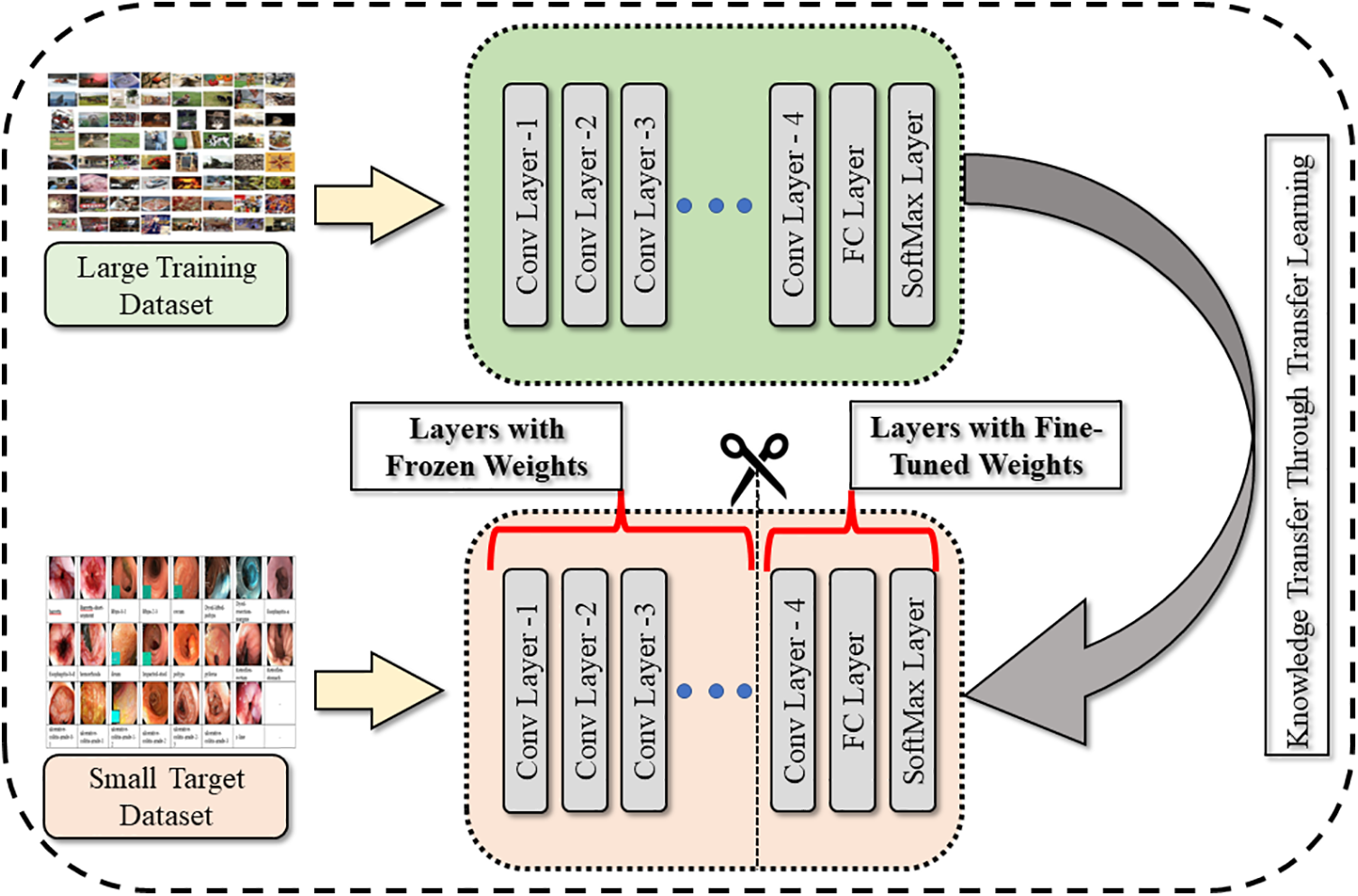
Figure 3: Generalization through transfer learning technique

3.4 Novelty: Proposed Features Selection

Feature selection is the operation of identifying a subset of appropriate features from a dataset’s larger set of features [35]. Feature selection improves model performance and data interpretation and reduces computational resources. Two feature selection algorithms are used to tackle the curse of dimensionality. Slime Mould Algorithm (SMA) is used to select important features in vector. S(Feat_AEvec) from Feat_AEvec extracted through the Stacked Auto-Encoder while the Marine Predator Algorithm (MPA) is used to extract selected features vector S(Feat_NNMobilevec) form Feat_NNMobilevec that is obtained through Nasnetmobile. S(Feat_AEvec) consists of 535 features whereas S(Feat_NNMobilevec) has 366 features.

The Slime Mold Algorithm is a feature selection technique influenced by nature and centered around slime mold behavior. The method employs a system of artificial particles that interact with one another to identify the ideal solution. SMA approaches the food according to the strength of the odor the food source spreads. The following equations describe the behavior of the method for slime mold:

Fs((i+1))={Fa(i)⟶+pb⟶.(X.⟶⟶Fa(i)−(Fb(i)⟶)),s<qpc⟶.F(i)⟶,s≥q(37)

Here, pb⟶ is the parameter ranging from −Gp to Gp. Also, pc⟶ is the parameter that goes from zero to one in descending order. i represents the iteration number. Moreover, Fa⟶ shows the location of the source that has the highest odour. F⟶ is the location where slime mould is located. Fa⟶ and Fb⟶ is a randomly selected food source at the initial time. Furthermore, X⟶ is the weight of mould, and q is derived as:

q=tan⁡|T(j)−EH|(38)

where j∈1, 2, 3, …, n and T(j) represents the fitness for F⟶. Gp is represented as:

Gp=tan⁡h−1(−(imax of i)+1)(39)

The weight of the mould is calculated mathematically as:

X⟶={1+q.log⁡(bd−T(j)bd−ωd+1), For some condition1−q.log⁡(bd−T(j)bd−ωd+1), Other than Condition(40)

q is the random number from the range zero to one. bd is the best fit for the current iteration, as ωd is the worst fit in the current iteration. The position updating is derived as:

Fs∗={rand.(boundupper−boundlower+boundlower),rand<yFa(i)⟶+pb⟶.(X.⟶Fa(i)⟶−(Fb(i)⟶)),s<q pc⟶.F(i)⟶,s≥q(41)

The Marine Predator Optimization Algorithm (MPO) is a metaheuristic optimization algorithm based on the foraging strategies of aquatic predators. MPO is an algorithm replicating the searching and preying behavior of deep-sea predatory animals such as sharks, orcas, and other ocean animals. Like most metaheuristic algorithms, MPA is a population-based approach in which the baseline answer is dispersed equally over the search area, as in the first experiment. Mathematically it is denoted by:

A0=A0+rand (Amax−Amin)(42)

Here, Amin is the lower bound, whereas Amax is the upper bound for variables. Rand stands for a randomly chosen vector ranging from zero to one. Based on the notion of survival of the fittest, it is considered that the most efficient hunters in nature are the strongest predators. As a result, the top predator is regarded as the most efficient means of generating an elite matrix. These elite matrices are meant to detect and track prey by leveraging their location data. Each element in the elite matrix denotes predators in a position to search for food. The second matrix is called the prey matrix, where each element represents the prey looking for food. Both matrices have r ×c dimensions where r shows the number of searching agents, whereas c represents the number of dimensions. At each iteration, the fittest predator substitutes the previous fittest predator.

There are three phases that MPA contains. Phase one is considered when a predator is moving faster than prey, and velocity is (V≥10). In this scenario, the best possible solution could be to stop updating the positions of predators. Mathematically it can be represented as:

if iteration< 13 of MaxIteration

Stpitr⟶=RandN−dist⟶⊗(eliteitr⟶−RandN−dist⟶⊕Pritr⟶), itr=1,…Ntotal

Pritr⟶=Pritr⟶+Const.RandN−dist⟶ ⊗ Stpitr⟶(43)

In this scenario, RandN−dist⟶ represents a normal distribution-generated vector of random integers simulating Brownian motion. The symbol “⊗” represents entry-wise multiplication. Prey is multiplied by the vector. RandN−dist⟶ to imitate its movement. RandN−dist is a vector of uniform random integers ranging from 0 to 1, whereas Const is a constant with a value of 0.5. This situation happens during the first one-third of iterations when the size of each step is large due to a greater capacity for exploration. iteration denotes the current iteration, and MaxIteration is the total number of possible iterations.

Phase two is considered as the unit velocity ratio when both prey and the predator have the same velocity, is (V≈10). In this phase, the prey is in exploitation mode and levy motion while the predator is in exploration mode with Brownian motion. For half of the population, this could be denoted by:

if iteration< 23 of MaxIteration

Stpitr⟶=RandL−dist⟶ ⊗ (eliteitr⟶− RandL−dist⟶ ⊕ Pritr⟶), itr=1,…Ntotal/2

Pritr⟶=Pritr⟶+Const.RandN−dist⟶ ⊗ Stpitr⟶(44)

Above, RandL−dist⟶ denotes the random number based on Levy distribution. For another half of the population, it is represented as:

Stpitr⟶=RandN−dist⟶ ⊗ ( RandN−dist⟶⊗eliteitr⟶− RandN−dist⟶ ⊕ Pritr⟶), itr=Ntotal/2,…Ntotal

Pritr⟶=eliteitr⟶+Const.Adpprm ⊗ Stpitr⟶(45)

whereas Adpprm= (1−iterationMaxiteration)(2(iterationMaxiteration)) is an adaptive control parameter to control the step size.

In phase three, the prey has a low velocity compared to the predator’s velocity. In low ratio velocity, the value will be (V=0.1). In this scenario, the best motion for the predator will be the Levy motion, as shown in the Eq. (46).

if iteration< 23 of MaxIteration

Stpitr⟶=RandL−dist⟶ ⊗ (RandL−dist⟶ ⊗eliteitr⟶− RandL−dist⟶ ⊕ Pritr⟶), itr=1,…Ntotal/2

Pritr⟶=eliteitr⟶+Const.RandN−dist⟶ ⊗ Stpitr⟶(46)

The reason for the change in marine predators’ behavior is the environmental changes inserted in the algorithm such as eddy formation and Fish Aggregating Device (FAD) manipulation. These two effects are denoted by:

Pritr⟶={Pritr⟶+Adpprm[bdup⟶+Rand⟶⊗(bdup⟶−bdlr⟶)]⊗Vecbin⟶,if  urand≤FADsPritr⟶+[FADs(1−urand)+](Prurand1⟶−Prurand2⟶) ,      if  urand>FADs(47)

Here, FADs = 0.20 represents the likelihood of FADs’ influence in the optimization procedure. A binary vector U is created by randomly creating a vector in the interval [0, 1] and replacing its elements with zero if they are less than 0.2 and with one if they are more than 0.2. The subscript r denotes a uniformly random number in the interval [0, 1]. The vectors bdup⟶ and bdlr⟶ contain the minimum and maximum dimensions. urand1 and urand2 denote the random indices of the prey matrix.

3.5 Novelty: Proposed Feature Fusion

The significance of feature fusion resides in its capacity to extract more meaningful information from numerous sources, which can lead to improved accuracy in classification, identification, and prediction [36]. Feature fusion can increase the resilience and reliability of machine learning systems, especially in cases when data is few or noisy, by merging complementary information from many sources. As stated before, two feature vectors, S(Feat_AEvec) and S(Feat_NNMobilevec), are retrieved from both networks utilized in this process; hence, it is important to merge both vectors to create a larger, more informative feature vector. A correlation extended serial technique is utilized to combine both vectors, which can be mathematically represented as follows:

Corel=∑(Rwi−Rw¯)(Xtj−Xt¯)∑(Rwi−Rw¯)2∑Xtj−Xt¯(48)

With this procedure, the features with a positive correlation (+1) are chosen into a new vector labeled. Vec3 and the features with a correlation value of 0 or −1 are added to Vec4. Then, the mean value of Vec4 is calculated as follows:

CorelT={Vecupd,Vec4≥0Ignore_feat,Vec4<0 (49)

Both vectors Vecupd and Vec4 are fused using the following formulation:

VecFused=(VecupdVec3)(50)

The final fused vector VecFused has 901 features.

4  Results and Discussion

The Hyper-Kvasir dataset is used for results and analysis purposes. The dataset contains 10662 images categorized into twenty-three classes. Data is highly imbalanced, so to cater to this issue, data is augmented. The augmented dataset contains 24,000 training images, while 520 are obtained for testing. The implementation uses a system with a core i7 Quad-core processor with 16 GB of RAM. Moreover, the system contains a graphics card with 4 GB of VRAM. MATLAB R2021a is used to achieve results.

4.1 Numerical Results

Results are shown in tabular and graphical form. Table 2 represents the results for the extracted features through Nasnetmobile that are given as input to the classifiers. The analysis shows that Wide Neural Network (WNN) has given the best overall accuracy of 93.90 percent, while Narrow Neural Networks, Bilayered Neural Networks, and Trilayered Neural Networks have the lowest accuracy of 93.10 percent. Time taken by WNN is also the highest among all other classifiers, while the lowest time cost is for Narrow Neural Networks. The confusion matrix for WNN is shown in Fig. 4.

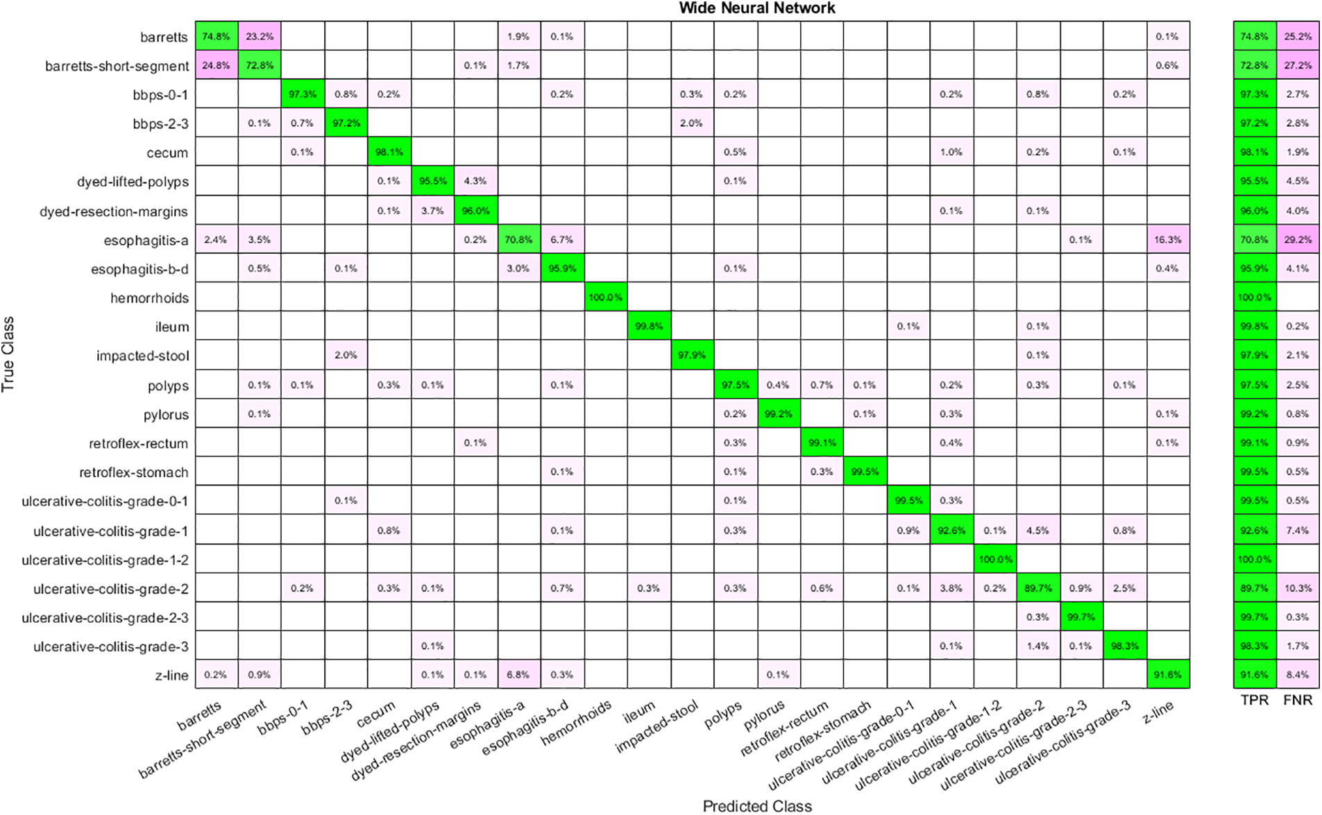
Figure 4: Confusion matrix for WNN using Nasnetmobile features

Similarly, Table 3 shows the results obtained by feeding the features extracted by implementing Stacked Auto-Encoders to classifiers. Analysis shows that WNN has the best performance with 80.50 percent accuracy, yet the time cost is also highest in the case of WNN and the lowest for Narrow Neural Networks. Moreover, the lowest accuracy is achieved by implementing a Narrow Neural Network. The confusion matrix for WNN is shown in Fig. 5.

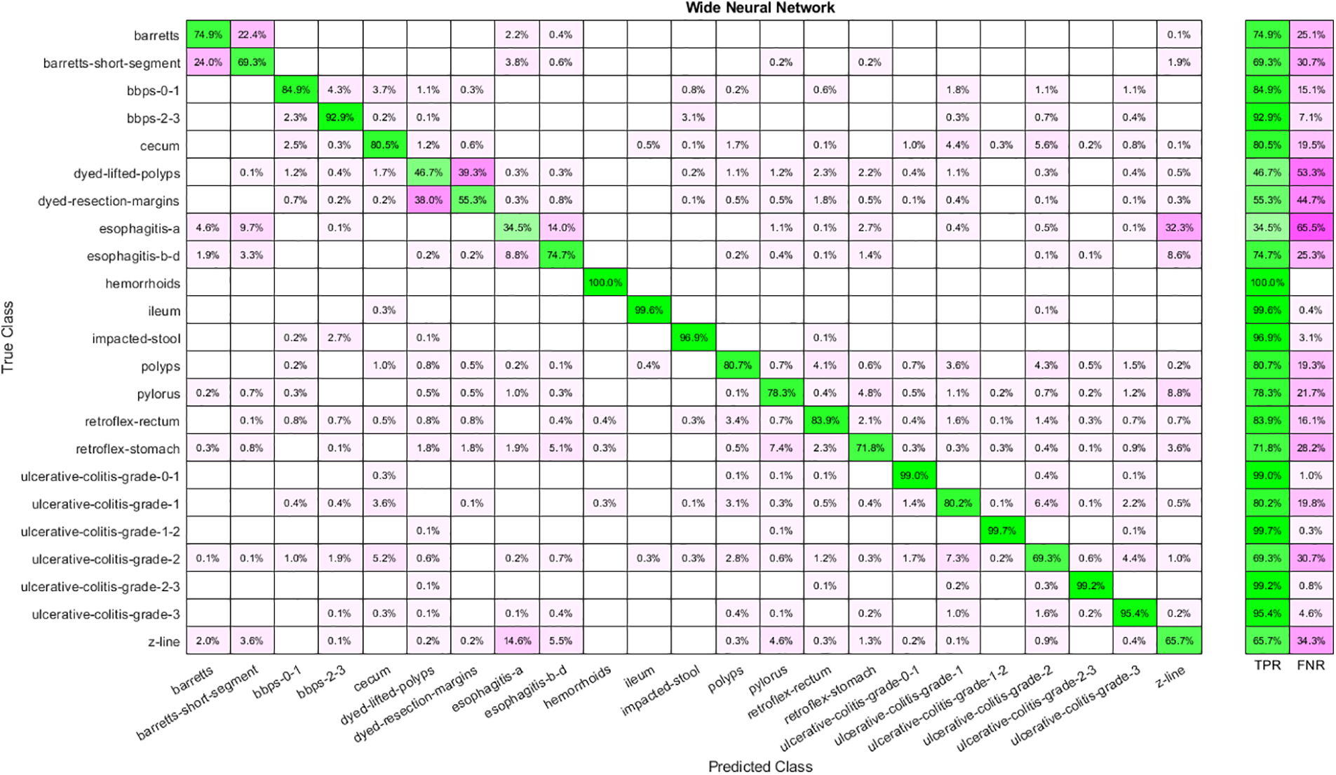
Figure 5: Confusion matrix for WNN using auto-encoder features

Feature selection has given reduced features from the feature vector extracted through Nasnetmobile. Table 4 shows the results for the selected features using the Marine Predator Algorithm (MPA). Selected features are given to the classifiers to obtain results. Analysis shows that WNN has the highest accuracy, 93.40, and the highest time cost. Furthermore, the lowest accuracy is obtained through a Trilayered Neural Network. A Narrow Neural Network has given the best time cost among all classifiers. The confusion matrix for WNN is shown in Fig. 6.

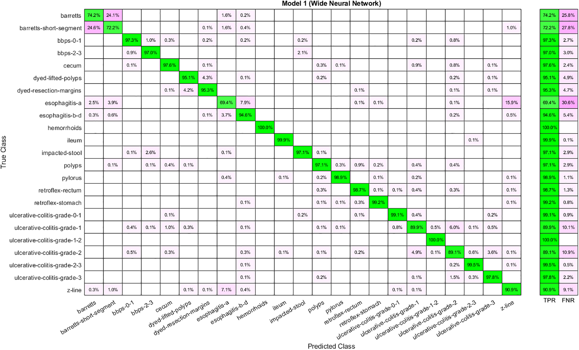
Figure 6: Confusion matrix for WNN using Nasnetmobile selected features

Table 5 shows the results achieved using the selected features from the Stacked Auto-Encoder. The features are selected using the Slime Mold Algorithm. WNN has the best performance as the accuracy achieved is 78.40 percent. Moreover, the time cost is highest for WNN and lowest for Narrow Neural Networks. In addition, Trilayered Neural Network has given the lowest accuracy. The confusion matrix for WNN is described in Fig. 7.

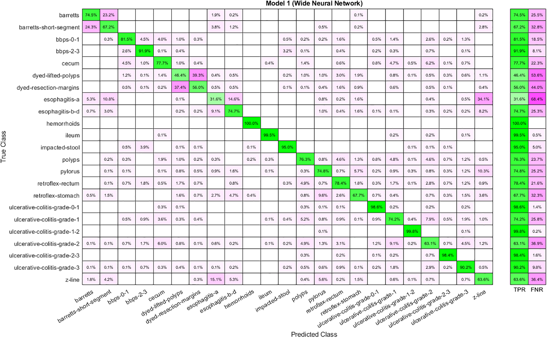
Figure 7: Confusion matrix for WNN using auto-encoder selected features

The best performance obtained using fused features is shown in Table 6. Features are given to ANNs and analyze the results. Analysis shows that the highest accuracy of 93.60 is achieved through WNN. Again, the time cost is high in the case of WNN, yet it is best for Narrow Neural Networks. Moreover, the lowest accuracy is obtained through a Narrow Neural Network. The confusion matrix for WNN is depicted in Fig. 8.

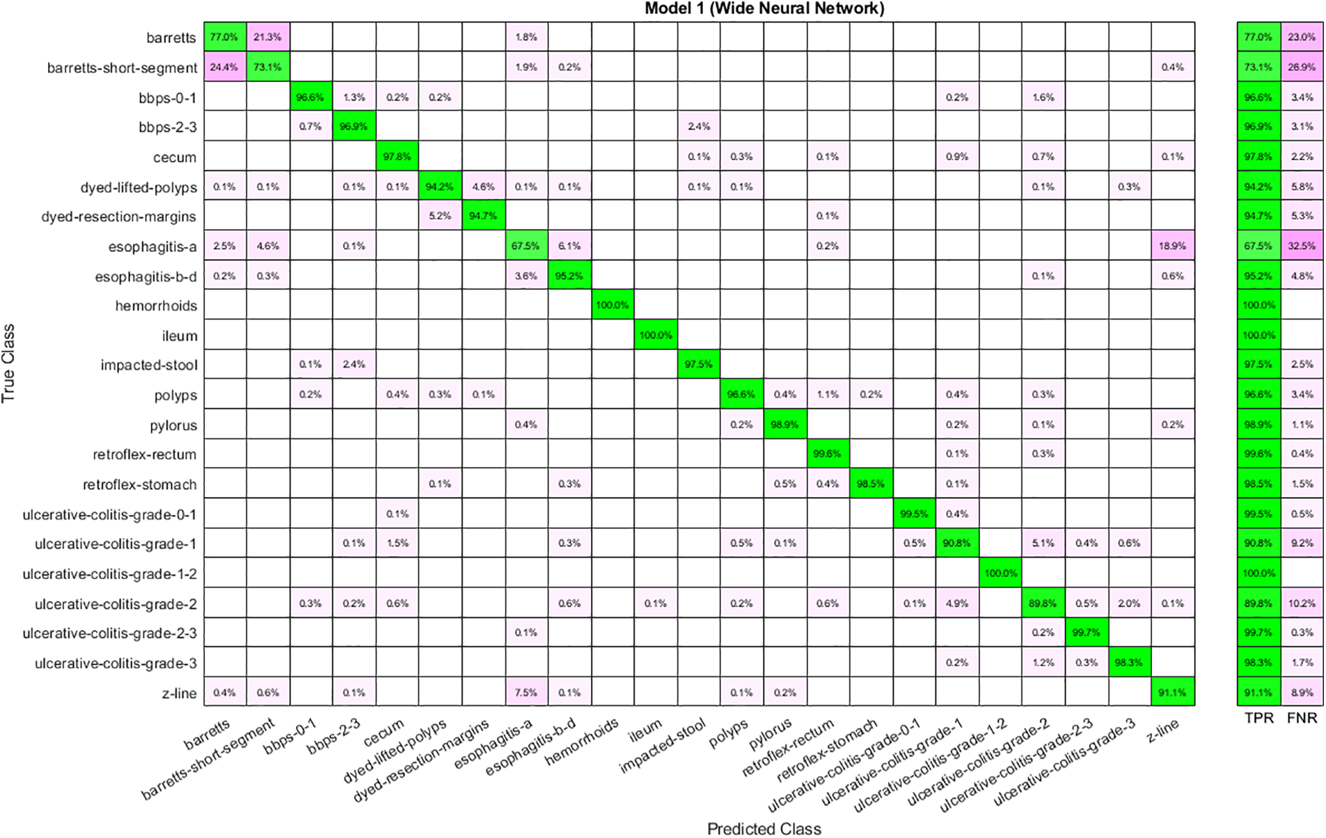
Figure 8: Confusion matrix for WNN using fused features

4.2 Graphical Results

This section shows the graphical representation of the results. Fig. 9 shows the bar chart for all classifiers using the proposed fusion approach. In this figure, each classifier’s accuracy is plotted with different colors, and Wide Neural Network shows the best accuracy of 93.8%, which is improved than the other classifiers. Fig. 10 shows the bar chart for the time cost for all classifiers after employing the final step of the proposed approach. Wide Neural Network (WNN) consumed the highest time of 772.93 (s), whereas the trilayered neural network spent a minimum time of 372.53 (s). Based on Figs. 10 and 11, it is observed that the wide neural network gives better accuracy but consumes more time due to additional hidden layers. Fig. 11 shows the time-based comparison of the proposed method. This figure shows that the time is significantly reduced after employing the feature selection step; however, a little increase occurs when the fusion step is performed. Overall, it is observed that the reduction of features impacts the computational time, which is a strength of this work.

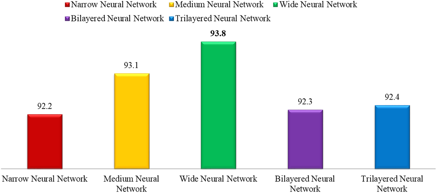
Figure 9: Accuracy bar for all selected classifiers using the proposed method

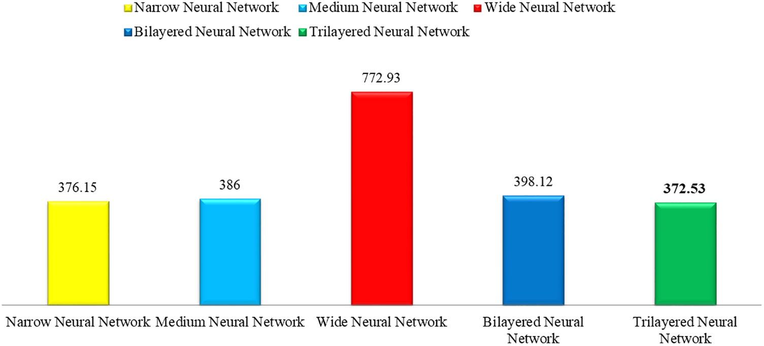
Figure 10: Time bar for classifiers used in the proposed methodology

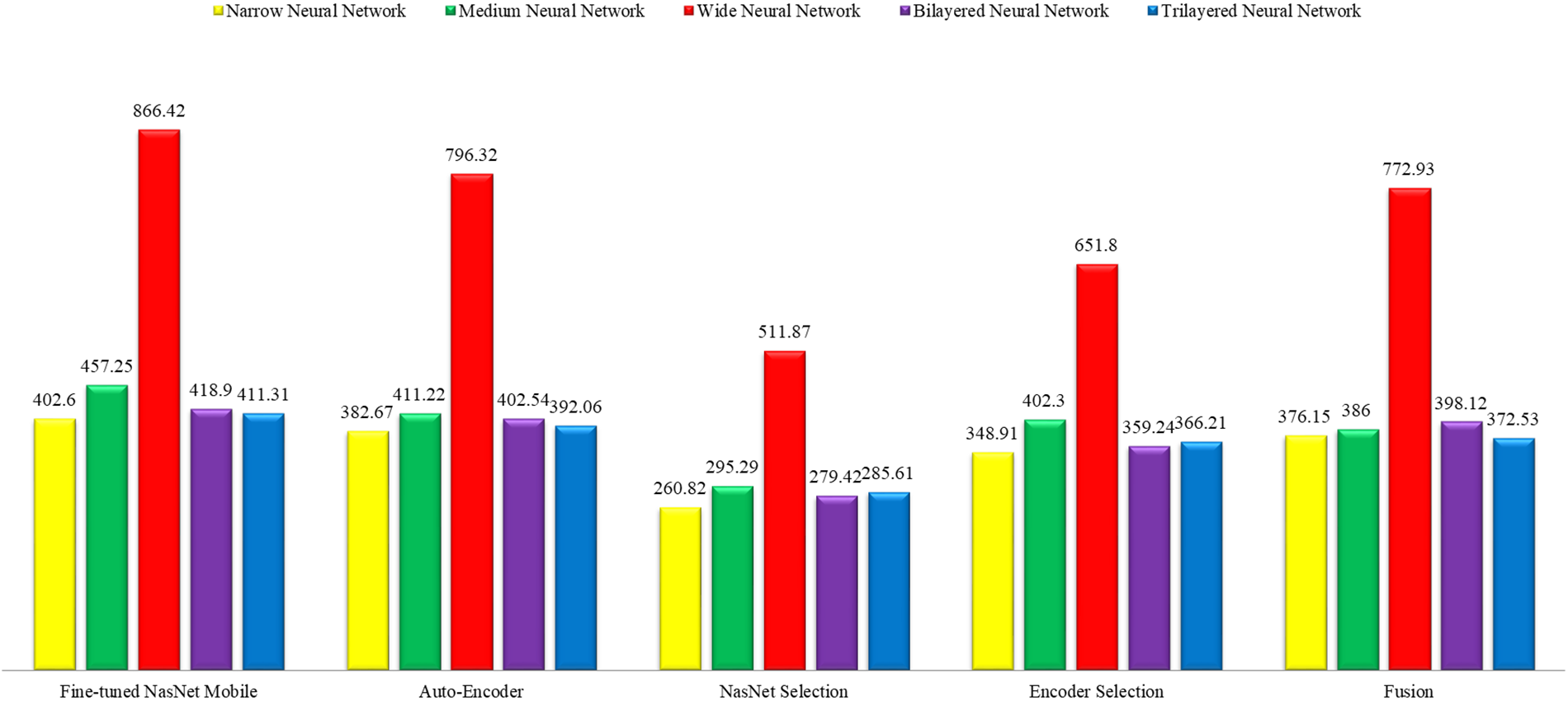
Figure 11: Overall time-based comparison among all classifiers using the proposed method

A detailed comparison is also conducted among all classifiers of the middle steps employed in the proposed method. Fig. 12 shows the insight view of this comparison. This figure shows that the original accuracy of the fine-tuned model NasNet Mobile is better, and the maximum is 93.9%; however, this experiment consumes more time, as plotted in Fig. 12. After the selection process, the accuracy is slightly reduced, but the time is significantly dropped. After the fusion process, it is noted that the difference in the classification accuracy of the wide neural network is just 0.1%, which is almost the same. Still, the time is significantly reduced, which is a strength of this work.

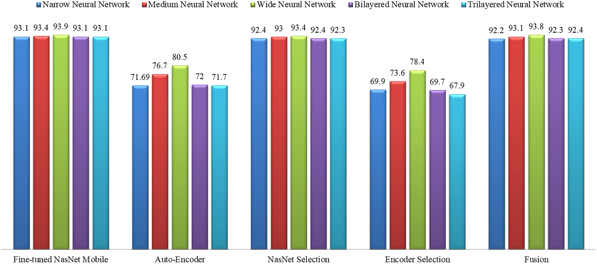
Figure 12: Accuracy comparison of all classifiers using all middle steps of the proposed method

LIME-based Visualization: Local Interpretable Model-Agnostic Explanations (LIME) [37] is a well-known technique for explainable artificial intelligence (XAI). It is a model-independent technique that may be used to explain the predictions of any machine learning algorithm, including sophisticated models like deep neural networks. LIME aims to produce locally interpretable models that approach the predictions of the original machine learning model in a limited part of the input space. Local models are simpler and easier to comprehend than the original model and can be used to explain specific predictions. The LIME approach generates a large number of perturbed versions of the input data and trains a local model on each disturbed version. Local models are trained to predict the output of the original model for each perturbed version and are then weighted according to their performance and resemblance to the original input. The final explanation offered by LIME is a mix of the weights of the local models and the most significant characteristics of each local model. An explanation can be offered to the user in the form of a heatmap or other visualization, as shown in Fig. 13, indicating which input data characteristics were most influential in forming the prediction.

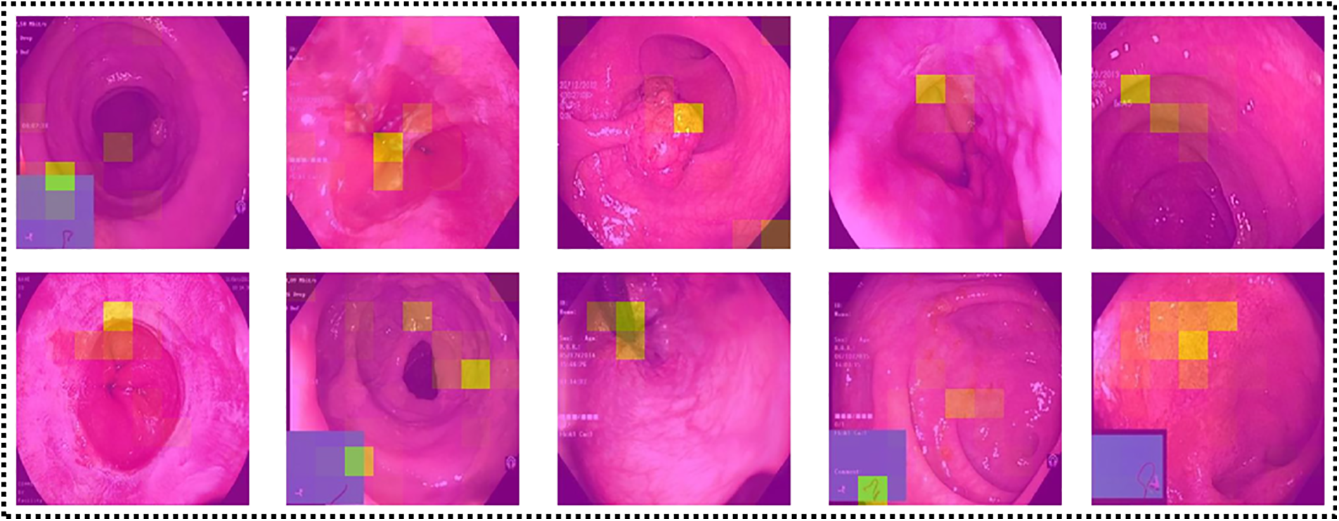
Figure 13: Explanation of network’s predictions using LIME

Fig. 14 shows the results of the fine-tuned Nasnetmobile deep model employed for infected region segmentation. The segmentation process employs the polyp images with corresponding ground truth images. This fine-tuned model is trained with static hyperparameters by employing original and ground truth images. After that, testing is performed to visualize a few images in binary form, as presented in Fig. 14. For the segmentation process, the weights of the second convolutional layers have been plotted and then converted into binary form.

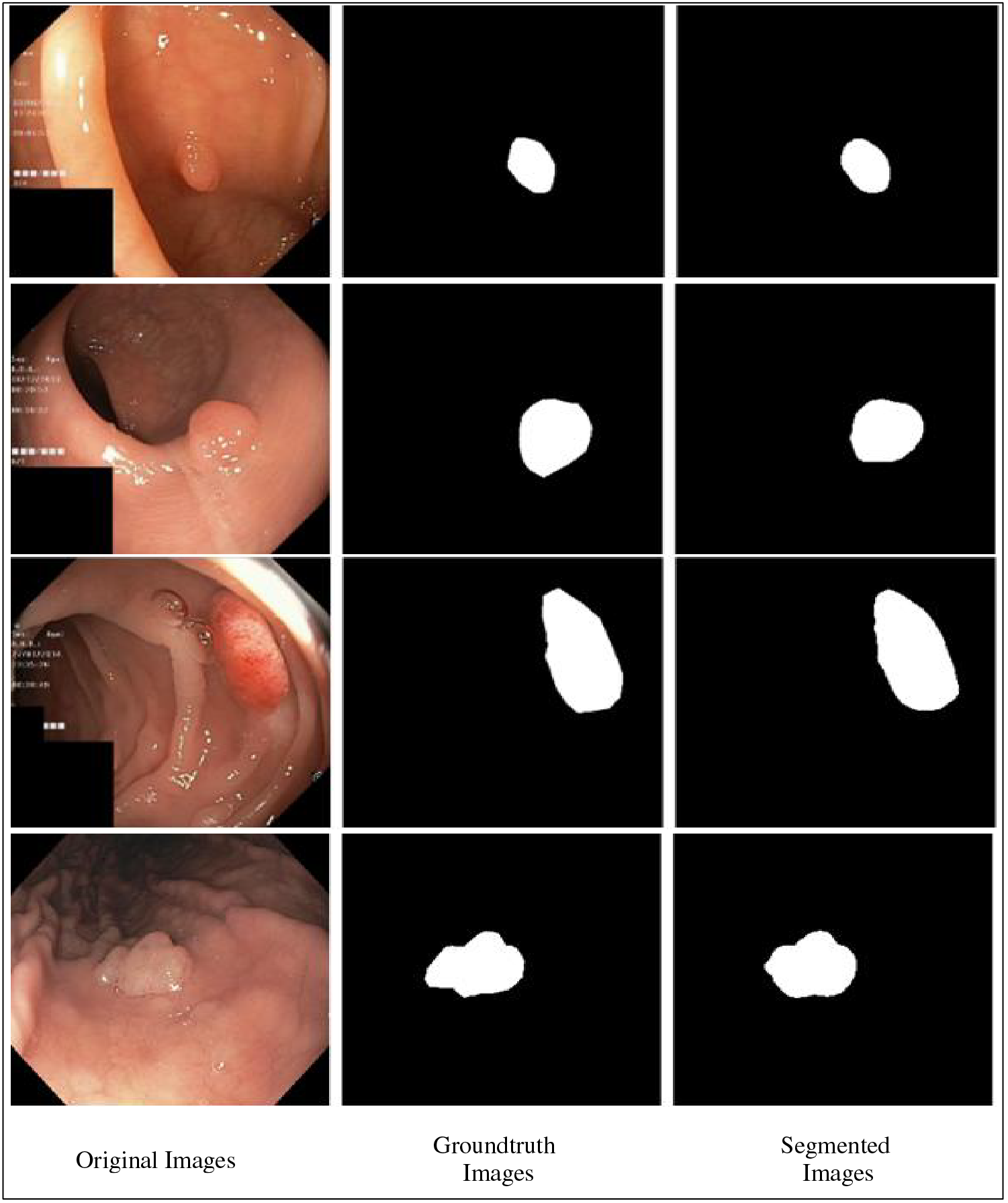
Figure 14: Proposed infection segmentation using fine-tuned Nasnetmobile deep model

Table 7 compares the results achieved in this article with recent state-of-the-art works. Reference [38] used self-supervised learning to classify the Hyper-Kvasir dataset. The authors used six classes and achieved the highest accuracy of 87.45. Moreover, reference [27] used the Hyper-Kvasir dataset to classify the gastrointestinal tract and obtained 73.66 accuracy. In the study, the authors only used fourteen classes. In addition, reference [23] achieved 63 percent accuracy for the macro and used all 23 classes. It is clear that the proposed method has outperformed the state-of-the-art methodologies in recent years and achieved the best accuracy of 93.80 percent. Moreover, the computational complexity of the proposed framework is O(Tn2+KC), where T denotes the middle steps, K are the parameters of deep learning architectures, and C denote the constant values.

5  Conclusion

Gastrointestinal tract cancer is one of the most severe cancers in the world. Deep learning models are used to diagnose gastrointestinal cancer. The proposed model uses Nasnetmobile and Auto-Encoder to extract deep features and is used as input for Artificial Neural Network classifiers. Moreover, feature selection techniques such as the Marine Predator Algorithm and Slime Mould Algorithm are implemented hybrid to cater to the curse of dimensionality problems. In addition, the selected features are fused and fed for classification. The results analysis shows that classification through features extracted from Nasnetmobile gives the best overall validation accuracy of 93.90. Overall, we conclude the following:

–   Data augmentation using contrast enhancement techniques can better impact the learning of deep learning models instead of using flip and rotation-based approaches.

–   Extracting encoders and deep learning features give better information on selected disease classes.

–   The selection of features in a hybrid fashion impacts the classification accuracy and reduces the time.

–   The fusion process improved the classification accuracy.

The drawbacks of this work are: i) segmentation of infected regions is a challenging task due to the change of lesion shape and boundary location; ii) manual assignment of hyperparameters of deep learning models is not a good way, and it always affects the learning process of a network. The proposed framework will be shifted to infected region segmentation using deep learning and saliency-based techniques. Moreover, we will opt for a Bayesian Optimization technique for hyperparameter selection. Although the proposed methodology has achieved the best outcomes, better accuracy may be achieved through different approaches in the future.

Acknowledgement: This work is supported by Princess Nourah bint Abdulrahman University Researchers Supporting Project, Princess Nourah bint Abdulrahman University, Riyadh, Saudi Arabia.

Funding Statement: This work was supported by “Human Resources Program in Energy Technology” of the Korea Institute of Energy Technology Evaluation and Planning (KETEP), granted financial resources from the Ministry of Trade, Industry & Energy, Republic of Korea (No. 20204010600090). Princess Nourah bint Abdulrahman University Researchers Supporting Project Number (PNURSP2023R387), Princess Nourah bint Abdulrahman University, Riyadh, Saudi Arabia.

Author Contributions: The authors confirm contribution to the paper as follows: study conception and design: A Haseeb, MA Khan, M Alhaisoni; data collection: A Haseeb, MA Khan, L Jamel, G Aldehim, and U Tariq; analysis and interpretation of results: MA Khan, J. Cha, T Kim, and U Tariq; draft manuscript preparation: Haseeb, MA Khan, L Jamel, G Aldehim, and J Cha; validation: J Cha, T Kim, and U Tariq; funding: J Cha, T Kim, L Jamel and G Aldehim. All authors reviewed the results and approved the final version of the manuscript.

Availability of Data and Materials: The Kvasir dataset used in this work is publically available. https://datasets.simula.no/kvasir/.

Conflicts of Interest: The authors declare that they have no conflicts of interest to report regarding the present study.

References

1. M. S. Ayyaz, M. I. U. Lali, M. Hussain, H. T. Rauf and B. Alouffi, “Hybrid deep learning model for endoscopic lesion detection and classification using endoscopy videos,” Diagnostics, vol. 12, no. 3, pp. 43, 2021. [Google Scholar] [PubMed]

2. J. S. Joseph and A. Vidyarthi, “Multiclass gastrointestinal diseases classification based on hybrid features and duo feature selection,” Journal of Biomedical Nanotechnology, vol. 19, no. 6, pp. 288–298, 2023. [Google Scholar]

3. S. Kashyap, S. Pal, G. Chandan, V. Saini and S. Chakrabarti, “Understanding the cross-talk between human microbiota and gastrointestinal cancer for developing potential diagnostic and prognostic biomarkers,” Seminars in Cancer Biology, vol. 5, no. 6, pp. 1–11, 2021. [Google Scholar]

4. S. Mohapatra, G. K. Pati, M. Mishra and T. Swarnkar, “Gastrointestinal abnormality detection and classification using empirical wavelet transform and deep convolutional neural network from endoscopic images,” Ain Shams Engineering Journal, vol. 14, no. 4, pp. 101942, 2023. [Google Scholar]

5. N. Sharma, A. Sharma and S. Gupta, “A comprehensive review for classification and segmentation of gastro intestine tract,” in 2022 6th Int. Conf. on Electronics, Communication and Aerospace Technology, Chenai, India, pp. 1493–1499, 2022. [Google Scholar]

6. F. Bray, J. Ferlay, I. Soerjomataram, R. L. Siegel and A. Jemal, “GLOBOCAN estimates of incidence and mortality worldwide for 36 cancers in 185 countries,” Cancer Journal for Clinicians, vol. 68, no. 11, pp. 394–424, 2018. [Google Scholar]

7. I. D. Apostolopoulos and T. A. Mpesiana, “COVID-19: Automatic detection from X-ray images utilizing transfer learning with convolutional neural networks,” Physical and Engineering Sciences in Medicine, vol. 5, no. 15, pp. 1, 2020. [Google Scholar]

8. I. Polaka, M. P. Bhandari, L. Mezmale, L. Anarkulova and V. Veliks, “Modular point-of-care breath analyzer and shape taxonomy-based machine learning for gastric cancer detection,” Diagnostics, vol. 12, pp. 491, 2022. [Google Scholar] [PubMed]

9. X. Pang, Z. Zhao and Y. Weng, “The role and impact of deep learning methods in computer-aided diagnosis using gastrointestinal endoscopy,” Diagnostics, vol. 11, pp. 694, 2021. [Google Scholar] [PubMed]

10. M. Owais, M. Arsalan, J. Choi, T. Mahmood and K. R. Park, “Artificial intelligence-based classification of multiple gastrointestinal diseases using endoscopy videos for clinical diagnosis,” Journal of Clinical Medicine, vol. 8, pp. 986, 2019. [Google Scholar] [PubMed]

11. V. Raut, R. Gunjan, V. V. Shete and U. D. Eknath, “Gastrointestinal tract disease segmentation and classification in wireless capsule endoscopy using intelligent deep learning model,” Computer Methods in Biomechanics and Biomedical Engineering: Imaging & Visualization, vol. 11, pp. 606–622, 2023. [Google Scholar]

12. H. Ko, H. Chung, W. S. Kang, K. W. Kim and Y. Shin, “COVID-19 pneumonia diagnosis using a simple 2D deep learning framework with a single chest ct image: Model development and validation,” Journal of Medical Internet Research, vol. 22, pp. e19569, 2020. [Google Scholar] [PubMed]

13. S. Ruder, “An overview of gradient descent optimization algorithms,” Applied Sciences, vol. 5, no. 2, pp. 1–11, 2016. [Google Scholar]

14. M. Farhad, M. M. Masud, A. Beg, A. Ahmad and L. Ahmed, “A review of medical diagnostic video analysis using deep learning techniques,” Applied Sciences, vol. 13, pp. 6582, 2023. [Google Scholar]

15. E. Sivari, E. Bostanci, M. S. Guzel, K. Acici and T. Ercelebi Ayyildiz, “A new approach for gastrointestinal tract findings detection and classification: Deep learning-based hybrid stacking ensemble models,” Diagnostics, vol. 13, pp. 720, 2023. [Google Scholar] [PubMed]

16. K. Sumiyama, T. Futakuchi, S. Kamba and N. Tamai, “Artificial intelligence in endoscopy: Present and future perspectives,” Digestive Endoscopy, vol. 33, pp. 218–230, 2021. [Google Scholar] [PubMed]

17. R. Zemouri, N. Zerhouni and D. Racoceanu, “Deep learning in the biomedical applications: Recent and future status,” Applied Sciences, vol. 9, pp. 1526, 2019. [Google Scholar]

18. P. Visaggi, N. de Bortoli, B. Barberio, V. Savarino and R. Oleas, “Artificial intelligence in the diagnosis of upper gastrointestinal diseases,” Journal of Clinical Gastroenterology, vol. 56, pp. 23–35, 2022. [Google Scholar] [PubMed]

19. Y. Song and W. Cai, “Visual feature representation in microscopy image classification,” in Computer Vision for Microscopy Image Analysis. Germany: Elsevier, pp. 73–100, 2021. [Google Scholar]

20. V. Maeda-Gutiérrez, C. E. Galvan-Tejada, L. A. Zanella-Calzada and J. M. Celaya-Padilla, “Comparison of convolutional neural network architectures for classification of tomato plant diseases,” Applied Sciences, vol. 10, pp. 1245, 2020. [Google Scholar]

21. H. Yu, R. Singh, S. H. Shin and K. Y. Ho, “Artificial intelligence in upper GI endoscopy-current status, challenges and future promise,” Journal of Gastroenterology and Hepatology, vol. 36, pp. 20–24, 2021. [Google Scholar] [PubMed]

22. M. N. Noor, M. Nazir, I. Ashraf, N. A. Almujally and S. Fizzah Jilani, “GastroNet: A robust attention-based deep learning and cosine similarity feature selection framework for gastrointestinal disease classification from endoscopic images,” CAAI Transactions on Intelligence Technology, vol. 1, no. 1, pp. 1–16, 2023. [Google Scholar]

23. H. Borgli, V. Thambawita, P. H. Smedsrud and S. Hicks, “HyperKvasir, a comprehensive multi-class image and video dataset for gastrointestinal endoscopy,” Scientific Data, vol. 7, pp. 283, 2020. [Google Scholar] [PubMed]

24. S. Igarashi, Y. Sasaki, T. Mikami, H. Sakuraba and S. Fukuda, “Anatomical classification of upper gastrointestinal organs under various image capture conditions using AlexNet,” Computers in Biology and Medicine, vol. 124, pp. 103950, 2020. [Google Scholar] [PubMed]

25. M. A. Gómez Zuleta, D. F. Cano Rosales, D. F. Bravo Higuera and J. A. Ruano Balseca, “Detección automática de pólipos colorrectales con técnicas de inteligencia artificial,” Rev Colomb Gastroenterol, vol. 36, no. 5, pp. 7–17, 2021. [Google Scholar]

26. M. H. Al-Adhaileh, E. M. Senan, W. Alsaade, T. H. H. Aldhyani and N. Alsharif, “Deep learning algorithms for detection and classification of gastrointestinal diseases,” Complexity, vol. 2021, no. 26, pp. 1–12, 2021. [Google Scholar]

27. P. H. Smedsrud, V. Thambawita, S. A. Hicks, H. Gjestang and O. O. Nedrejord, “Kvasir-capsule, a video capsule endoscopy dataset,” Scientific Data, vol. 8, pp. 142, 2021. [Google Scholar] [PubMed]

28. A. Faramarzi, M. Heidarinejad, S. Mirjalili and A. H. Gandomi, “Marine predators algorithm: A nature-inspired metaheuristic,” Expert Systems with Applications, vol. 152, no. 21, pp. 113377, 2020. [Google Scholar]

29. M. Zafar, J. Amin, M. A. Anjum, G. A. Mallah and S. Kadry, “DeepLabv3+-based segmentation and best features selection using slime mould algorithm for multi-class skin lesion classification,” Mathematics, vol. 11, no. 4, pp. 348–364, 2023. [Google Scholar]

30. Y. T. Kim, “Contrast enhancement using brightness preserving bi-histogram equalization,” IEEE Transactions on Consumer Electronics, vol. 43, pp. 1–8, 1997. [Google Scholar]

31. K. R. Mohan and G. Thirugnanam, “A dualistic sub-image histogram equalization based enhancement and segmentation techniques for medical images,” in 2013 IEEE Second Int. Conf. on Image Information Processing (ICIIP-2013), Shimla, India, pp. 566–569, 2013. [Google Scholar]

32. G. Kumar and P. K. Bhatia, “A detailed review of feature extraction in image processing systems,” in 2014 Fourth Int. Conf. on Advanced Computing & Communication Technologies, Mumbai, India, pp. 5–12, 2014. [Google Scholar]

33. P. Zhou, J. Han, G. Cheng and B. Zhang, “Learning compact and discriminative stacked autoencoder for hyperspectral image classification,” IEEE Transactions on Geoscience and Remote Sensing, vol. 57, pp. 4823–4833, 2019. [Google Scholar]

34. X. Qin and Z. Wang, “NASNet: A neuron attention stage-by-stage net for single image deraining,” Applied Sciences, vol. 22, no. 4, pp. 1–18, 2019. [Google Scholar]

35. J. Li, K. Cheng, S. Wang, F. Morstatter and R. P. Trevino, “Feature selection: A data perspective,” ACM Computing Surveys (CSUR), vol. 50, no. 2, pp. 1–45, 2017. [Google Scholar]

36. A. Majid, M. Yasmin, A. Rehman, A. Yousafzai and U. Tariq, “Classification of stomach infections: A paradigm of convolutional neural network along with classical features fusion and selection,” Microscopy Research and Technique, vol. 83, no. 6, pp. 562–576, 2020. [Google Scholar] [PubMed]

37. S. Khedkar, V. Subramanian, G. Shinde and P. Gandhi, “Explainable AI in healthcare,” in 2nd Int. Conf. on Advances in Science & Technology (ICAST), NY, USA, pp. 1–6, 2019. [Google Scholar]

38. T. Nguyen-DP, M. Luong, M. Kaaniche and A. Beghdadi, “Self-supervised learning for gastrointestinal pathologies endoscopy image classification with triplet loss,” Sesnors, vol. 4, no. 1, pp. 1–21, 2023. [Google Scholar]

39. X. Wu, C. Chen, M. Zhong and J. Wang, “HAL: Hybrid active learning for efficient labeling in medical domain,” Neurocomputing, vol. 456, no. 21, pp. 563–572, 2021. [Google Scholar]