Missing Value Imputation for Radar-Derived Time-Series Tracks of Aerial Targets Based on Improved Self-Attention-Based Network

1  Introduction

In combat situational awareness and understanding, the air battlefield has been the focal point of attention. The aerial target is a crucial element in the air battlefield situation. The radar early warning system detects and tracks targets, generating and storing abundant time-series track data in the information processing center encompassing a wealth of general information and latent knowledge. Currently, data mining on radar-derived time-series tracks of aerial targets (RTT-AT) has provided favorable support in target behavior pattern analysis [1–3], maneuver identification [4–6], activity and intention discrimination [7–9], abnormal behavior detection [10–13], and threat estimation [14–17].

However, missing values are pervasive in RTT-AT due to radar terminal malfunction, packet loss during data transmission, and storage loss [18]. These missing values undermine the completeness and balance, leading to degradation in the performance of data-driven learning tasks. Therefore, imputing sensible values for missing data points in RTT-AT is a crucial fundamental task.

Intuitively, the imputation of missing values RTT-AT can be formulated as a problem of multivariate time series imputation (MTSI), which involves estimating missing values in a time series with multiple attributes. In the domain of MTSI, utilizing the statistical properties of either a single sample or the entire dataset to impute missing values is a highly classical approach, including techniques such as mean imputation, median imputation, and more. Extensive research has demonstrated that this method can lead to considerable bias [19]. Moreover, various in-sample methods are commonly employed for missing value imputation, including nearest-neighbor-based methods [20,21] and matrix-decomposition-based methods [22,23]. These methods rely solely on the information available within the given sample, but ignoring information from other instances within the set may result in performance limitations. Cross-sample methods, such as expectation-maximization-based [24,25] and constraint-based methods [26,27], aim to address this limitation by leveraging information from multiple samples within the dataset. Expectation-maximization-based methods can be sensitive to initial parameter values, model assumptions, and outliers. Additionally, the computational complexity is high due to the need for multiple iterations. Constraint-based methods are challenging to define, have a high risk of failure, and are computationally expensive. Overall, the majority of traditional methods outlined above necessitate assumptions concerning missing mechanisms and distribution, and these assumptions can lead to bias.

In recent years, data-driven deep learning techniques have garnered significant attention and have extensively been applied in various domains, showcasing their robust capabilities and vast potential. Specifically, these techniques have demonstrated remarkable achievements in computer vision, natural language processing, bioinformatics, and beyond [28–31]. Drawing inspiration from these groundbreaking works, numerous scholars within the realm of MTSI have embraced deep learning techniques to learn and harness the plenary sample information comprehensively and aimed at achieving superior imputation performance. Notably, a preponderance of these pioneering efforts is rooted in the utilization of gated recurrent neural networks (GRNNs). Recurrent Neural Networks (RNNs) occupy a pivotal position when it comes to the processing of sequence data. Their unique structure endows them with the remarkable capability to capture dependencies within sequences. However, vanilla RNNs are susceptible to the pernicious problems of gradient vanishing and long-term memory failure, which can severely undermine their performance. The GRNNs represent an enhancement over the vanilla RNN architecture. It introduces a gating unit integrated within the network’s structure, which endows the model with greater control over the influence of past information on the current output. This added level of control facilitates the capture of time dependencies, spanning both short-term and long-term durations. Furthermore, the GRNN can also capture interdependencies among different attributes within a multivariate series [32].

GRNN-based imputation methods can be categorized into two distinct classes: unidirectional GRNN-based models and bidirectional GRNN-based imputation models [33–36]. The former employs a strategy that predicts the next value in the sequence based on the preceding observations. This approach heavily relies on the contextual relevance of the missing value’s past moments to predict the missing value. On the other hand, bidirectional GRNNs exhibit superior performance by utilizing both forward and backward hidden layers. This architecture enables the extraction of the long-range context dependencies from both past and future time steps of missing values. By leveraging temporal dependencies in both directions, bidirectional GRNNs outperform their unidirectional counterparts. Multi-directional Recurrent Neural Networks (M-RNN) and Bidirectional Recurrent Imputation for Time Series (BRITS) are the most representative bidirectional GRNN methods [35,36]. The former treats missing values as constants, while the latter treats missing values as variables with the RNN graph. Additionally, M-RNN does not consider correlations among attributes, whereas BRITS does. All the aforementioned GRNN-based imputation methods are subject to the limitations of recursive networks, which involve sequential operations on time steps that can be time-consuming and memory-intensive. Moreover, their capacity to capture long-term dependencies decreases as the length of the sequence increases. Additionally, most of these models are autoregressive, which makes them susceptible to the compound error problem.

The typical missing patterns that occurred in RTT-AT are referred as random missing at altitude attribute (RM-ALT) and random missing at all attributes (RM-ALL). Due to the difference in the generation mechanism, the two differ significantly in the distribution of missing values from the random missing (RM) mode which is the concern of general time series imputation works. Specifically, with the RM pattern, missing values occur randomly at any time in any attribute; in RM_ALT, missing values occur randomly at any time, specific to the altitude attribute; and in RM-ALL, missing values appear randomly at any time, resulting in all attributes being unobserved at that moment.

Hence, when the traditional imputation methods designed for addressing RM are directly applied to tackle the two missing patterns in RTT-AT, their underlying assumptions become inapplicable, potentially leading to increased data bias. In addition, conventional deep learning imputation methods based on GRNN are vulnerable to cumulative errors and long-term dependency loss problems due to the network structure, leading to performance bottlenecks. The self-attention mechanism, being data-driven and autoregressive, can address the aforementioned issues. This paper proposes a model to impute missing values of RTT-AT based on an improved self-attention-based network. The contributions include:

(1) This paper posits RTT-AT data imputation as a problem of imputing multivariate time series. A novel non-autoregressive imputation model to minimize imputation loss is proposed to tackle the typical missing patterns. The imputation loss enables the training of the non-autoregressive model, facilitating its focus on learning the missing properties rather than entirely reconstructing the observations. Non-autoregressive models with minimizing imputation loss as the learning objective perform significantly better than models (whether autoregressive or non-autoregressive) with minimizing reconstruction loss as the learning objective.

(2) The designed non-autoregressive imputation model comprises two cascades of probabilistic sparse diagonally masking self-attention (PSDMSA) units and a weight fusion unit. In PSDMSA, the probabilistic sparsity is introduced to emphasize the importance of prominent dot-product pairs and simultaneously decrease computational complexity. Moreover, the diagonal masking ensures more significant attention to the temporal dependencies and attribute correlations between time steps. The fusion unit can automatically learn the weights of two units’ outputs by considering temporal and attribute correlations and missing information to obtain a better representation. The design enables enhanced capability to capture missing patterns and improved imputation quality with fewer parameters and reduced training time costs.

(3) A series of comparison and ablation experiments are conducted to evaluate the effectiveness of our proposed model. The experimental findings indicate that the method outperforms other approaches in imputing missing values of RTT-AT regardless of variations of missing rate. Additionally, while the method’s performance decreases as the missing rate increases, this decrease is relatively limited. The ablation experiments demonstrate the efficiency and effectiveness. The structure of the following sections is as follows: Section 2 presents an overview of the preliminary, Section 3 introduces the detail of the model proposed, whereas Sections 4 and 5, respectively, present the experiments and conclusion.

2  Preliminary

In this section, the definitions and formal descriptions of multivariate time series, time series missing value imputation, related works on time series missing value imputation and typical missing patterns in RTT-AT are presented in Sections 2.1, 2.2, 2.3, and 2.4, respectively.

2.1 Multivariate Time Series

A time series is a collection of values obtained from a period of continuous time measurements. Formally, a collection of timestamps T=(t0,t1,…,tn) and a time series X={xt0,xt1,…,xtn}T are first defined, X consists of n observations; Xti={xti0,xti1,…,xtid}, the observation of X at the timestamp ti, contains d attributes; when d>1, X is a multivariate time series (MTS). In this paper, the elements of the MTS are real numbers.

2.2 Time Series Missing Value Imputation

The binary missing mask matrix M={mt0,mt1,…,mtn} is defined to represent the locations of missing values in MTS X. It contains n timestamps and d attributes, and mti=(mti1,mti,…,2mtid) denotes the mask vector corresponding to xti, and

mtij={0,1,xtijis\,missing\,valuextijis observed value(1)

The aim of time series missing value imputation is to employ the imputation model to substitute every missing component of X with a justifiable value, ultimately achieving a complete time series X^.

2.3 Related Works on Time Series Missing Value Imputation

In general, based on the difference in the number of samples used, time series missing value imputation methods can be divided into two types: in-sample methods and cross-sample methods. The former uses information from the current sample only, while the latter uses information from the current sample and other samples during the training or testing phase.

2.3.1 In-Sample Methods

Statistical-Characteristic-Based Methods

Imputation methods based on statistical characteristics are simple and easy to apply. The most commonly used statistical characteristics are the mean value [37,38] and median value [39]. In the mean imputation approach, missing values are filled in by average of all the observed values of the attribute they are in. On the other hand, the median imputation utilizes the median value of observations. One salient issue with statistical-characteristic-based methods is that when the missing values are large in number, all those missing values are replaced by the same value. This can result in significant changes to the distribution’s shape. Simulation studies have demonstrated that mean imputation and median imputation yield highly biased parameter estimates [40].

Matrix-Decomposition-Based Methods

The matrix-decomposition-based imputation methods use a matrix/tensor approach to imputing missing values in multivariate time series. Literature [23] proposes a multivariate time series imputation method based on autoregressive matrix decomposition to solve the problem of temporal and spatial series data reconstruction in structural health monitoring of civil engineering applications. Literature [22] proposes an imputation model for missing values in traffic congestion time series based on joint matrix decomposition. The model estimates the missing values using temporal and spatial information while jointly modeling the characteristics of traffic congestion patterns. Literature [41] proposes a low-rank autoregressive tensor decomposition framework for solving the problem of missing values in spatial-temporal traffic time series. Experimental results demonstrate its effectiveness on several real-world traffic datasets and multiple missing scenarios. The approaches based on matrix decomposition have low computational complexity and can handle large datasets. However, they are typically only suitable for static data and rely on a limited amount of information, necessitating strong assumptions such as low rank [36].

Nearest-Neighbor-Based Methods

Nearest-neighbor-based methods estimate missing values by finding the nearest neighbors (determined by a set distance criterion). The method involves finding the nearest neighbors of the missing value through other attributes and then updating the missing value with the average of these nearest neighbors. Among the available methods, considering local similarity, some use the last observed value instead of the missing value [42]. Literature [21] analyses the use of k-nearest neighbor as the imputation method. Results indicate that missing data imputation based on k-nearest neighbor outperforms the embedding methods used in C4.5 and CN2. Literature [20] proposes an imputation algorithm that considers a fixed set of nearest neighbors. Experiments on datasets with real world missing attribute values demonstrate its effectiveness [20]. Since the missing values are estimated from actual observations, the nearest-neighbor-based imputation methods avoid distortion of the distribution. However, applying these methods to large datasets can be time-consuming. Additionally, the choice of K value can significantly impact the results.

2.3.2 Cross-Sample Methods

Expectation-Maximization-Based Methods

The expectation maximization (EM) algorithm consists of two steps. In the E-step, the expectation of the complete data sufficient statistics is calculated based on the observations and current parameter estimates. In the M-step, the parameter estimates are updated using the maximum likelihood method. The algorithm iterates until the convergence criteria are met. Based on the final parameter estimates and observations, the imputation of each missing value can be calculated. Literature [25] investigated and compared the imputation performance of the combination of expectation maximization and genetic algorithms under several different types of datasets. The study showed that the EM algorithm performs well when there is little correlation between the attributes. Literature [24] proposes a method for imputing missing values in multivariate time series using the EM algorithm under the assumption of a normal distribution. Experimental results show good imputation performance when the missing rate is less than 5%. However, when the missing rate is greater than 10%, the performance declines significantly. The EM imputation algorithm estimates the missing values based on actual observations, which can avoid distortion in the distribution. However, EM also has the following problems: First, the choice of initial values, model assumptions, and outliers can have a large impact on the results. Meanwhile, the EM algorithm is computationally intensive due to the need for multiple iterations. Additionally, the model run may encounter problems if any other sample is not closely related to the entire dataset’s manner [43].

Constraint-Based Methods

Constraint-based methods are used to discover rules in the dataset and estimate missing values. In time series imputation, similarity rules, such as differential dependence or comparable dependence, are commonly used to study the distance and similarity between timestamps as well as values [44,45]. Literature [27] proposes to extensively enrich the similarity neighbors through the tolerance of similarity rules to small variations, which leads to higher imputation accuracy than the conventional nearest-neighbor-based method. Literature [26] proposes a missing value imputation algorithm for streaming data based on data speed change constraints. Experiments on real data show its effectiveness. More high-level constraints can be set through a graph structure [46]. These constraints are commonly used to impute the qualitative values of events in a time series. Constraint-based methods are effective in cases where the data within the sample is highly continuous or when certain patterns are satisfied. However, multivariate time series typically do not conform to these simple rules, and more intricate rules tend to apply only to data in a specific domain [47].

Machine-Learning-Based Methods

Many researchers have applied machine learning methods to time series missing value imputation, inspired by their outstanding performance in time series identification and prediction. Literature [48] utilizes decision trees to identify horizontal segments of the dataset and then imputes missing values using similarity and attribute correlations. The experimental results show that the technique has significant advantages based on statistical analyses such as confidence intervals. Literature [49] proposes two imputation methods: a single method based on a multilayer perceptron (MLP) trained using different learning rules, and a multiple method based on a combination of a MLP and the k-nearest neighbors technique. The results, considering different performance metrics, show that both methods improve the level of automation and data quality compared to the traditional one. Literature [50] assessed the imputation performance of different random forest (RF) algorithms using numerous datasets under various missing data regimes. The results indicate that RF is generally robust, and its performance improves with increasing attribute relevance. Moreover, the performance remains good even at medium-to-high level of missingness. Most machine-learning-based imputation methods have good generality and scalability, but they may not be able to extract deeper features during computation due to algorithmic limitations.

Deep-Learning-Based Methods

Recently, deep learning techniques that can mine deep hidden features have been utilized for time series missing value imputation. Recurrent neural networks are commonly used for these methods due to their ability to handle sequential information. Currently, the two most representative methods are M-RNN and BRITS. M-RNN is a multinomial recurrent neural network that imputes within data streams and estimates between data streams. Experimental results on five real world medical datasets show that M-RNN significantly improves the estimate quality of missing values and performs robustly [35]. BRITS learns the missing values of the bidirectional recursive dynamical system without making any assumptions. The estimates are treated as variables of the RNN graph and can be efficiently updated in backpropagation. Experimental results on three real-world datasets from different domains show that the method effectively improves the performance of imputation, as well as downstream classification and regression [36]. The structure of RNNs makes them time-consuming and memory-intensive. Additionally, the autoregressive nature of the model negatively affects the imputation results due to compound errors. Some researchers have proposed the use of generative adversarial networks (GANs) for time series imputation. However, it is important to note that the majority of GAN-based methods still rely on RNNs [51–53]. These methods cannot eliminate certain drawbacks of RNN-based methods. Additionally, GAN-based models are challenging to train, and GANs suffer from non-convergence and pattern collapse due to their learning objective [54].

2.4 Typical Missing Patterns in RTT-AT

According to Little and Rubin’s definition, there are three types of missing generation mechanisms in MTS [35]:

1. Missing Completely at Random (MCAR), where the probability of a target attribute being missing is not influenced by any observed and unobserved attributes, in simpler terms; the missingness occurs randomly.

2. Missing at Random (MAR), where the probability of missing the target attribute is related to the observed attributes but not the unobserved variables.

3. Missing not at Random (MNAR) refers to scenarios where the likelihood of a target attribute being missing is connected to unobserved attributes, indicating a non-random characteristic in the missingness.

Moreover, attributes refer to the characteristics or features of a MTS. When all the missing values pertain to the same attribute, the missing is called single-valued missing (SM). Furthermore, if the missing values belong to different attributes, it is called arbitrary missing (AM).

This paper centered on RTT-AT acquired and stored by early warning detection radar terminals. Detection radar can be divided into height finder radar, two-dimensional radar, and three-dimensional radar based on the number of dimensions in which targets’ position information can be detected. The two-dimensional radar can determine aerial targets’ bearing and distance while collaborating with the height finder radar to identify aerial targets and attain their bearing, distance, and altitude. The three-dimensional radar can simultaneously acquire aerial targets’ bearing, distance, and altitude information. While the three-dimensional radar offers remarkable functional integration and high-performance capabilities, it comes at a significant cost. Conversely, the cheap and easy-to-operate two-dimensional radar and the height finder radar remain the most extensively employed in early warning and detection. Therefore, the scenario of coordinated detection by the two-dimensional radar and the height finder radar is considered, where the two-dimensional radar typically acquires the target’s azimuth and distance information initially, while the height finder radar obtains the altitude data. After undergoing pre-processing operations such as coordinate transformation, the radar-derived trajectory data has three attributes: longitude, latitude, and altitude. In this cooperative working mode, the following two typical missing patterns are considered, as shown in Fig. 1: (1) random missing at altitude attribute (RM-ALT) caused by malfunction of the height finder radar, operator setting errors, etc.; (2) random missing at all attributes (RM-ALL) caused by malfunction of the two-dimensional radar, communication loss, etc.

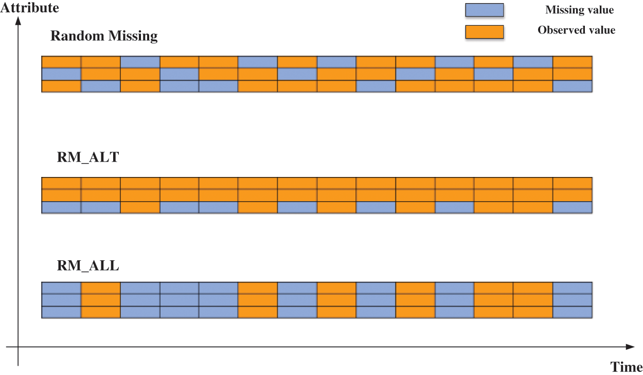
Figure 1: The distribution of three missing patterns

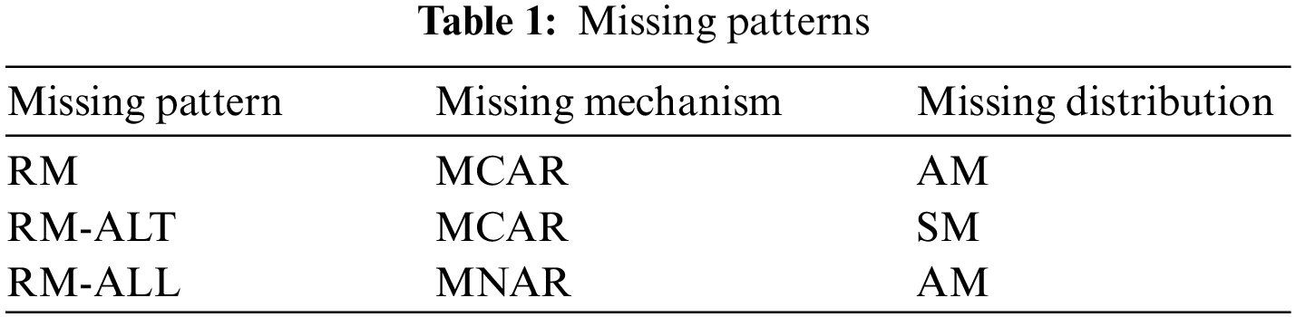
The missing pattern typically addressed by general time series imputation methods is random missing (RM), in which the missing values occur randomly and are uncorrelated among all attributes. Nevertheless, the two missing patterns in RTT-AT exhibit distinct characteristics from RM. In RM_ALT, the missing values occur randomly only at any moment in the altitude attribute and not in the other attributes. Additionally, in RM_ALL, the missing values occur randomly at any moment, and missingness with missingness in the altitude dimension is correlated with missingness in both the other dimensions. Furthermore, when there are missing values, the values of all attributes at that moment in time are unobserved. A summary of the above three modes is shown in Table 1, and Fig. 1 shows the differences in the distribution of the three missing patterns. In Fig. 1, each row denotes an attribute of the track, and each column denotes the values at a time step. The orange squares denote observed values in the track data, while the light blue ones represent missing values.

3  Methodology

The methodology consists of two parts: (1) the missing value imputation workflows presented in Section 3.1 and (2) the network based on PSDMSA presented in Section 3.2.

3.1 Missing Value Imputation Workflows

The missing value imputation workflows for RTT-AT are shown in Fig. 2, which contains two stages, data processing and imputation model learning.

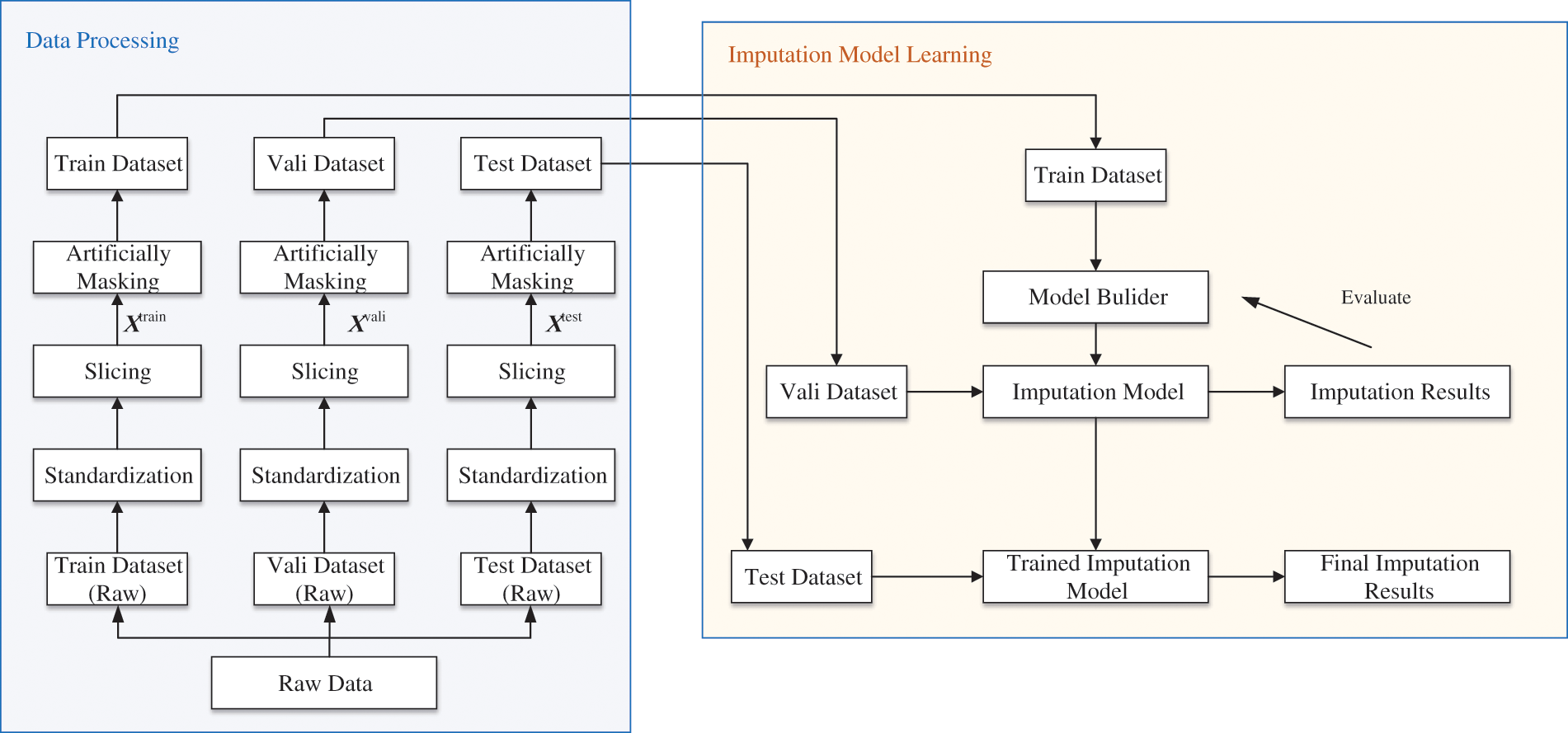
Figure 2: Missing value imputation workflows

During the data processing phase, the initial step involves partitioning the raw multivariate time-series radar track data into dedicated training, validation, and testing sets according to a predefined split ratio. Subsequently, a standardization operation is executed on the data within the training, validation, and testing subsets. This step is crucial as it eliminates disparities in measurement units and scales across different attributes, ultimately improving the model’s accuracy in filling missing values. Moreover, standardizing the data also improves the model’s convergence properties, reducing potential oscillations caused by disparities in data scales during the optimization process. The process of standardization can be represented as follows:

xi,j,kSt=xi,j,k−xjminxjmax−xjmin(2)

In Eq. (2), xi,j,k represents raw values for the k-th sample under the j-th class of attributes, at the i-th sampling point, xjmin and xjmax represent smallest and largest values, respectively, observed in the j-th attribute dimensions across all samples within the training set, xi,j,kSt represents standardized data.

Due to their vast and variable nature in length, radar-derived track time series present a challenge for effective processing using deep learning models. A methodological approach is adopted to address this issue. Specifically, a non-interlaced sliding window of identical length is utilized to segment the track data. This segmentation ensures that the resulting sliced dataset exhibits uniformity in sample length, enhancing its amenability to deep learning-based processing. For visual clarification, the precise operational procedure of this slicing method is graphically elucidated in Fig. 3.

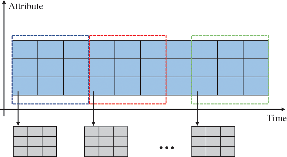
Figure 3: Fixed-length sliding window slicing process

Subsequently, observations are randomly masked to generate incomplete samples with missing values in conformance with the predetermined proportion of missingness. Additionally, a corresponding mask matrix is produced for these missing values according to Eq. (1). Together, the complete samples, incomplete samples, and the mask matrix compose a comprehensive dataset that serves as the foundation for imputation model learning and performance evaluation.

During the imputation model learning phase, the work addresses the challenge of imputing missing values in RTT-AT. This is achieved by treating it as a supervised learning problem, where we aim to learn relationships between observed data points to minimize the loss between missing values and corresponding predicted values and capture missing patterns. The training set plays a crucial role in developing the imputation model, calculating loss, and updating parameters through an optimization process guided by a specific loss function. Meanwhile, the validation set serves a dual purpose: fine-tuning the hyper-parameters of the model and evaluating its initial performance and effectiveness. This provides valuable insights into the model’s potential performance. Following the completion of training and learning, the test set samples are utilized to comprehensively evaluate the trained model’s imputation capabilities and generalizability, employing relevant evaluation metrics to quantify its performance.

To delve into more specific details, let us examine the notation and learning objective used in our imputation model. The unaltered complete sample before artificial masking as X and the resulting incomplete sample after the introduction of artificial masking as Xinput. In Xinput, missing values are filled with zeroes due to computational requirements and ease of model handling. Correspondingly, Minput represents the mask matrix indicating the locations of missing values about Xinput. The input matrix for the imputation model is derived by concatenating Xinput with Minput, and the model’s output is the predicted completed sample, denoted as Xfinal, where the missing values have been aptly filled. The learning objective of the model is to minimize the Mean Absolute Error (MAE) between the actual missing values and their predicted counterparts, which can consciously direct the imputation model to “predict” the missing values precisely and to learn the missingness pattern better. It is named as imputation loss (IL). Eqs. (3) and (4) give the expression for the IL:

LOSSMAE(output,target,mask)=∑d=1D∑t=1T|(output−target)⊙mask|td∑d=1D∑t=1Tmasktd(3)

IL=LOSSMAE(Xfinal,X,(1−Minput))(4)

where D represents the number of attributes and T represents the number of time steps. ⊙ represents element-wise product.

3.2 The PSDMSA-Based Imputation Network

The network designed comprises two cascaded PSDMSA units and a weight fusion unit, as depicted in Fig. 4. This section will detail the functions and structures of each of these units.

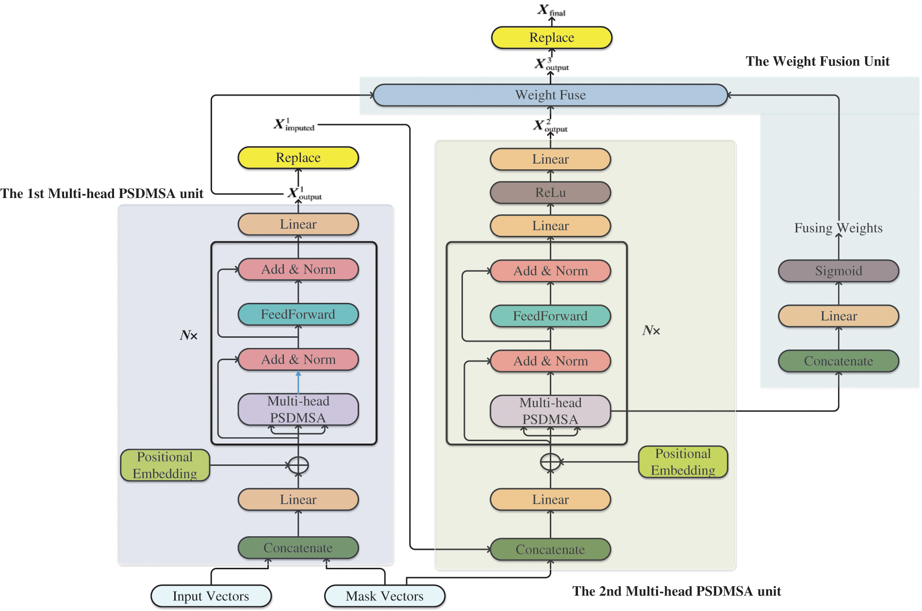
Figure 4: The PSDMSA-based network

3.2.1 PSDMSA

The vanilla self-attention mechanism was initially proposed by Vaswani and has subsequently found extensive application in natural language processing, computer vision, and sequence modeling [55]. Precisely, for a given sequence x∈RT×dmodel, it is mapped into three matrices: Q, K, and V:

Q=xWQ,K=xWK,V=xWV(5)

where WQ∈Rdmodel×dk,WK∈Rdmodel×dk,WV∈Rdmodel×dv represent parameter matrices for linear transformations. Q, K, and V dimensions are dk, dk and dv. Then, the attention map is acquired through the computation of the scaled dot-product between Q and K, and a nonlinear function Softmax is utilized to obtain the attention weight A. At final, A and V are multiplied directly to get output. Eq. (6) shows the process:

A(Q,K,V)=Softmax(QKTdk)V(6)

Softmax(zi)=ezi∑c=1Cezc(7)

Due to vanilla self-attention’s long-tailed distribution structure, dot-product operations on queries and keys show that most dot-product pairs have a limited contribution, and only a few pairs have a dominant role. Therefore, to emphasize the importance of prominent dot-product pairs and simultaneously decrease computational complexity, the probabilistic sparsity is introduced into the vanilla self-attention mechanism of the imputation model [56]. Furthermore, the negative infinity values are assigned to the diagonal position of the probabilistic-sparse attention map to ensure greater attention to the temporal dependencies and feature correlations between time steps. This improved self-attention mechanism is referred to as probabilistic sparse diagonal masking self-attention (PSDMSA), as shown in Fig. 5:

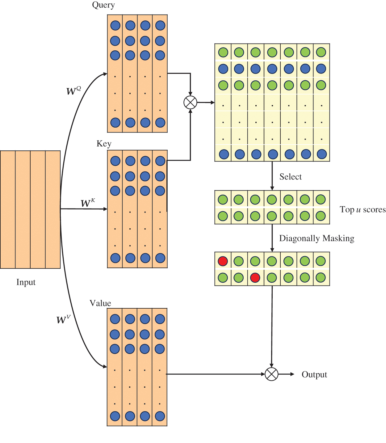
Figure 5: The PSDMSA

In Fig. 5, the rectangle in the top right corner illustrates the vanilla attention map. The green circle denotes a notable correlation between the query and the key at this location. In contrast, the blue circle signifies no significant correlation. PSDMSA takes Q, K, and V as inputs consistent with the vanilla self-attention mechanism. The distinction lies in the fact that:

(1) PSDMSA evaluates the importance of queries based on the Kullback-Leibler divergence before performing the dot-product operation and selects only the top-u essential queries for the subsequent operation. The remaining queries are directly assigned to the mean value, thus effectively reducing the number of dot-product calculations.

(2) The elements at the diagonal of the attention map are set to negative infinity (set to −1×109 in practice).

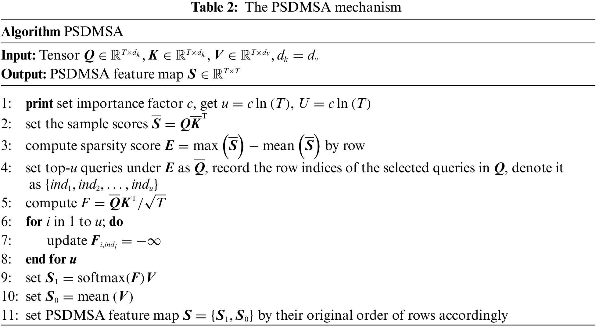
The specific process is shown in Table 2. The dimension of the PSDMSA output is equal to the output of the vanilla self-attention mechanism. However, PSDMSA samples only u queries to compute the attention score. In addition, the diagonal masking operation causes the output of PSDMSA to have a value of 0 for the elements on the diagonal position.

Subsequently, to enhance information extraction efficiency, PSDMSA is expanded to multi-head PSDMSA:

Multi−head PSDMSA(x)=Concat(head1,head2,…,headi,…,headh)(8)

where headi=PSDMSA(Q,K,V), h denotes the number of heads, and Concat represents a concatenating operation.

3.2.2 Positional Embedding

In the initial Transformer design, temporal order was not considered. Vaswani implemented positional embedding to provide positional information to the input vector to the Transformer [55]. Positional embedding is expressed as:

pe(pos,2i)=sin⁡(pos/(100002i/dmodel))(9)

pe(pos,2i+1)=cos⁡(pos/(100002i/dmodel))(10)

where pos denotes location information for each moment, dmodel denotes the dimension of the output of the first linear layer, and i is the dimension.

3.2.3 Feed-Forward Network

The feed-forward network consists of two cascaded fully connected layers and a ReLu function as shown in Eq. (11):

FeedForward(x)=W2max(0,W1x+b1)+b2(11)

where W1∈Rdmodel×dhidden, b1∈Rdhidden, W2∈Rdhidden×dmodel and b2∈Rdmodel.

3.2.4 The First Multi-Head PSDMSA Unit

e=[Concat(Xinput,Minput)We+be]+pe,We∈R2D×dmodel,be∈Rdmodel(12)

z={Feed Forward(Multi−headPSDMSA(e))}N(13)

Xoutput1=zWz+bz,Wz∈Rdmodel×D,bz∈RD(14)

Ximputed1=Minput⊙Xinput+(1−Minput)⊙Xoutput1(15)

In the first unit, as shown in Eq. (12), the input feature vector Xinput and missing value mask vector Minput are concatenated as the actual input. Subsequently, the actual input is mapped into a vector of dimension dmodel by a linear layer. This resulting vector is summed with the positional embedding pe, which has the same dimension, to obtain the embedding vector e. e is then fed into N stacked layers of the multi-head PSDMSA blocks and feed-forward network to obtain z, as shown in Eq. (13). Subsequently, in Eq. (14), a linear layer transfers z into Xoutput1 of dimension D, note that Xoutput1 and Xinput are of equal dimensions. Finally, in Eq. (15), the missing values in Xinput are replaced with values in Xoutput1 at corresponding positions to obtain the completed vector Ximputed1, ⊙ represents element-wise multiplication.

3.2.5 The Second Multi-Head PSDMSA Unit

e′=[Concat(Ximputed1,Minput)We′+be′]+pe,We′∈R2D×dmodel,be′∈Rdmodel(16)

z′={FeedForward(Multi−headPSDMSA(e′))}N(17)

Xoutput2=ReLu(z′Wz′+bz′)Wf+bf,Wz′∈Rdmodel×D,bz′∈RD,Wf∈RD×D,bf∈RD(18)

In the second unit, the feature vector obtained by concatenating the Ximputed1 learned in the first unit and Minput is used as the input. Similar to Eq. (12), Eq. (15) projects the input from 2D dimension to dmodel dimension, and then directly adds the result with the pe to get e′. Subsequently, e′ is fed into N stacked layers of the multi-head PSDMSA blocks and feed-forward network to obtain z′ as shown in Eq. (17), and Eq. (18) conducts two linear transformations and a single nonlinear transformation z′ to obtain Xoutput2. Xoutput1 and Xoutput2 are combined using a learnable weight that is acquired through the weight fusion unit.

3.2.6 The Weight Fusion Unit

A¯=1h∑i=1hAi(19)

θ=sigmoid(Concat(A¯,Minput)Wθ+bθ),Wθ∈R(T+D)×D,bθ∈RD(20)

Xoutput3=(1−θ)⊙Xoutput1+θ⊙Xoutput2(21)

Xfinal=Minput⊙Xinput+(1−Minput)⊙Xoutput3(22)

The fusion unit’s function is to automatically learn the weights of Xoutput1 and Xoutput2 by considering temporal and attribute correlations and missing information to obtain a better representation Xoutput3. A¯ in Eq. (19) is averaged from multi-head attention weights Ai outputted by the last layer of the second multi-head PSDMSA unit. Subsequently, Eq. (20) takes the feature vector concatenated by A¯ and Minput as the reference to obtain the weights θ(∈(0,1)T×D) using one linear layer and a nonlinear Sigmoid function. Eq. (21) fuses the Xoutput1 and Xoutput2 by weights θ to get Xoutput3. Finally, missing values in Xinput are replaced with values in Xoutput3 at corresponding positions to produce the final imputed vector Xfinal.

4  Experimental Results and Analysis

4.1 Experimental Data

In this study, the data come from the complete RTT-AT records in the same area obtained and kept by a radar team in the air situation simulation system. This team comprised a two-dimensional radar and a height finder radar. Moreover, the records cover six typical target activities: reconnaissance, police patrol, refueling, AWAC, attack, and retreat.

The dataset consists of 12000 time-series tracks with a sampling frequency of 10 Hz. The lengths of tracks range from 1052 to 8534. After undergoing a coordinate transformation process, each time-series track in the dataset is represented by three attributes: longitude (in degrees), latitude (in degrees), and altitude (in km). Fig. 6 offers visual examples of RTT-AT records, allowing readers to understand better the nature of the data being analyzed. Each example demonstrates the temporal evolution of longitude, latitude, and altitude for a specific target track.

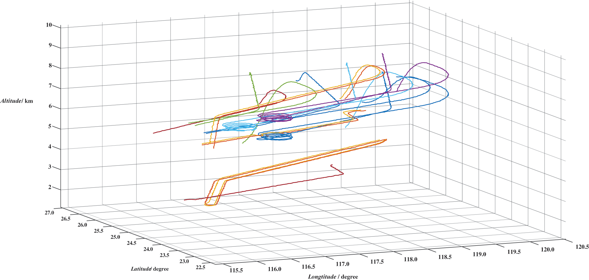
Figure 6: Examples of RTT-AT

A set of procedures designed to preprocess the data are conducted to prepare the initial data for training the imputation model. These procedures are outlined below. First, data slicing is performed, dividing all track data into segments of length 500 without overlapping. This slicing approach results in a total sample size of 166000.

Next, all data samples are standardized by attribute, ensuring each attribute has a mean of 0 and a standard deviation of 1. This step creates the standardized sample set, essential for maintaining consistent scales across different attributes during model training.

Lastly, the missing values of various patterns and rates are introduced into the standardized sample set, forming two distinct datasets: DataRM−ALT and DataRM−ALL. In DataRM−ALT, the missing rate is defined according to Eq. (23). It is set as 5%, 10%, 15% and 20%.

missing rate=NummissingD×T(23)

where Nummissing denotes the number of missing values, T denotes the sliced time-series length, and D denotes the number of attributes.

Samples in DataRM−ALL have RM-ALL, the missing rate is set as 10%, 20%, 30%, 40%, 50% and 60%.

4.2 Performance Evaluation Metrics and Experimental Setup

In this paper, three widely used metrics are utilized to assess the imputation performance of our model: mean absolute error (MAE), root mean square error (RMSE), and mean relative error (MRE). These metrics comprehensively evaluate imputation accuracy by calculating the differences between actual missing values and their imputed counterparts. Specifically, Eqs. (24)–(26) define the mathematical formulations of MAE, RMSE, and MRE, respectively. By examining these metrics, we aim to gain insights into the strengths and weaknesses of our imputation models, ensuring a rigorous and thorough evaluation process.

MAE(output,target,mask)=∑d=1D∑t=1T|(output−target)⊙(1−mask)|∑d=1D∑t=1T(1−masktd)(24)

RMSE(output,target,mask)=∑d=1D∑t=1T(((output−target)⊙(1−mask))2)td∑d=1D∑t=1T(1−masktd)(25)

MRE(output,target,mask)=∑d=1D∑t=1T|(output−target)⊙(1−mask)|∑d=1D∑t=1T|target⊙(1−mask)|td(26)

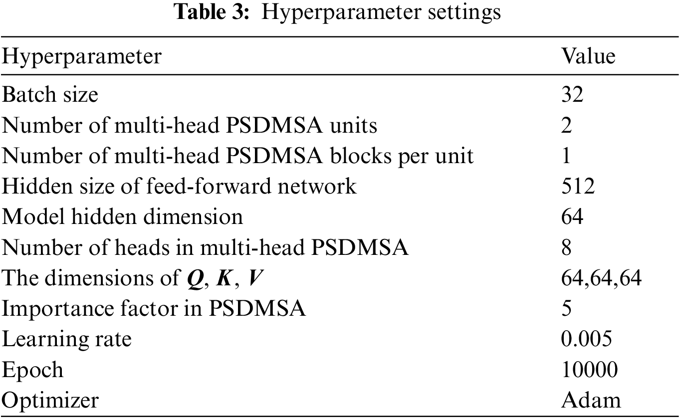
A batch size of 32 is used for model training, validation, and testing, which strikes a balance between computational efficiency and generalization performance. An early stopping mechanism that monitors the training loss is employed to prevent overfitting and ensure timely convergence. Training is halted, and the best model parameters are saved if the loss does not decrease after 100 consecutive epochs, indicating potential stagnation in the learning process. The chosen optimizer for our model is Adam. Specific hyperparameters associated with the Adam optimizer, such as the learning rate, are detailed in Table 3. This table provides a comprehensive overview of the hyperparameter settings used in our proposed model, facilitating reproducibility and further fine-tuning if needed.

To ensure consistent and reproducible results, all experiments were conducted on a single computer platform with specific hardware and software configurations. The platform was equipped with an Intel i5 10200 CPU, 32 GB of memory, and an NVIDIA GeForce RTX 2060 GPU, providing a balanced computational environment for our research. And the deep learning framework used is Pytorch.

4.3 Imputation Performance for RM-ALT

In Sections 4.3 and 4.4, our proposed method is compared to several current imputation methods, including:

(1) Zero Imputation (Zero). Imputing missing values with zero; (2) Mean Imputation (Mean) [37]. Imputing missing values with corresponding mean values from the training set; (3) Median Imputation (Median) [37]. Imputing missing values with corresponding median values from the training set; (4) K-Nearest-Neighbors (KNN) [57]. Imputing missing values with the weighted average of k neighbors by using a k-nearest neighbor algorithm; (5) Random Forest (RF) [50]. Observations in the vicinity of the missing point are used as features to train high-fit random trees to predict the missing values; (6) M-RNN [35]. Imputing missing values using multi-directional recurrent neural networks; (7) BRITS [36]. Imputing missing values using bidirectional uncorrelated RNN; (8) Transformer: Imputing missing values using a vanilla Transformer.

The results of different imputation methods for RM-ALT at varying missing rates appear in Table 4.

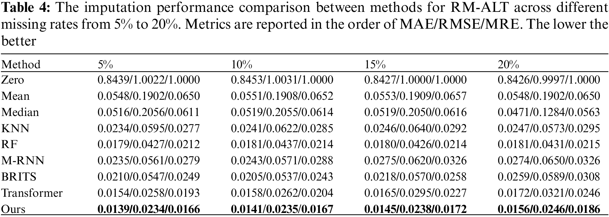
Firstly, the Zero method demonstrates the poorest performance among all considered methods. Secondly, KNN and RF consistently outperform Median and Mean methods at all missing rates, emphasizing their efficacy in imputing missing data over imputation methods based on statistical characteristics. Specifically, the RF method exhibits a substantial reduction of 65.3%, 79.2%, and 65.3% in MAE, RMSE, and MRE values, respectively, compared to the Median method when dealing with a missing rate of 20%. Moreover, our results indicate that the M-RNN method performs inferior to both KNN and RF. On the other hand, the BRITS method, which also relies on GRNNs, yields lower MAE and RMSE than the KNN method for missing rates of 5%, 10%, and 15%. However, at a missing rate of 20%, BRITS experiences a higher MAE value than KNN but maintains a lower RMSE. These findings imply that the BRITS method presents less bias than KNN at specific missing values. Nevertheless, its overall performance remains inferior to that of RF across varying missing rates.

On the contrary, irrespective of the missing rate, our proposed model shows lower MAE, RMSE, and MRE values than others. This implies that it possesses more extraordinary imputation ability when facing RM-ALT. When the missing rate is 5%, our proposed method yielded a 22.3% decrease in MAE, a 45.2% decrease in RMSE, and a 21.7% decrease in MRE relative to RF; when the missing rate is 20%, the respective decreases were 13.8%, 42.9%, and 13.5%. These results reveal that our method exhibits significant improvement in RMSE, which indicates that imputing missing values using this method does not result in significant deviations at specific missing points.

4.4 Imputation Performance for RM-ALL

Table 5 presents the imputation performance of different imputation models in addressing RM-ALL across varying missing rates, comprehensively comparing our proposed model against eight other methods. Notably, the table reveals that the missing rate in the RM-ALL scenario does not significantly impact the relative performance between models. This observation underscores the effectiveness and robustness of our proposed model.

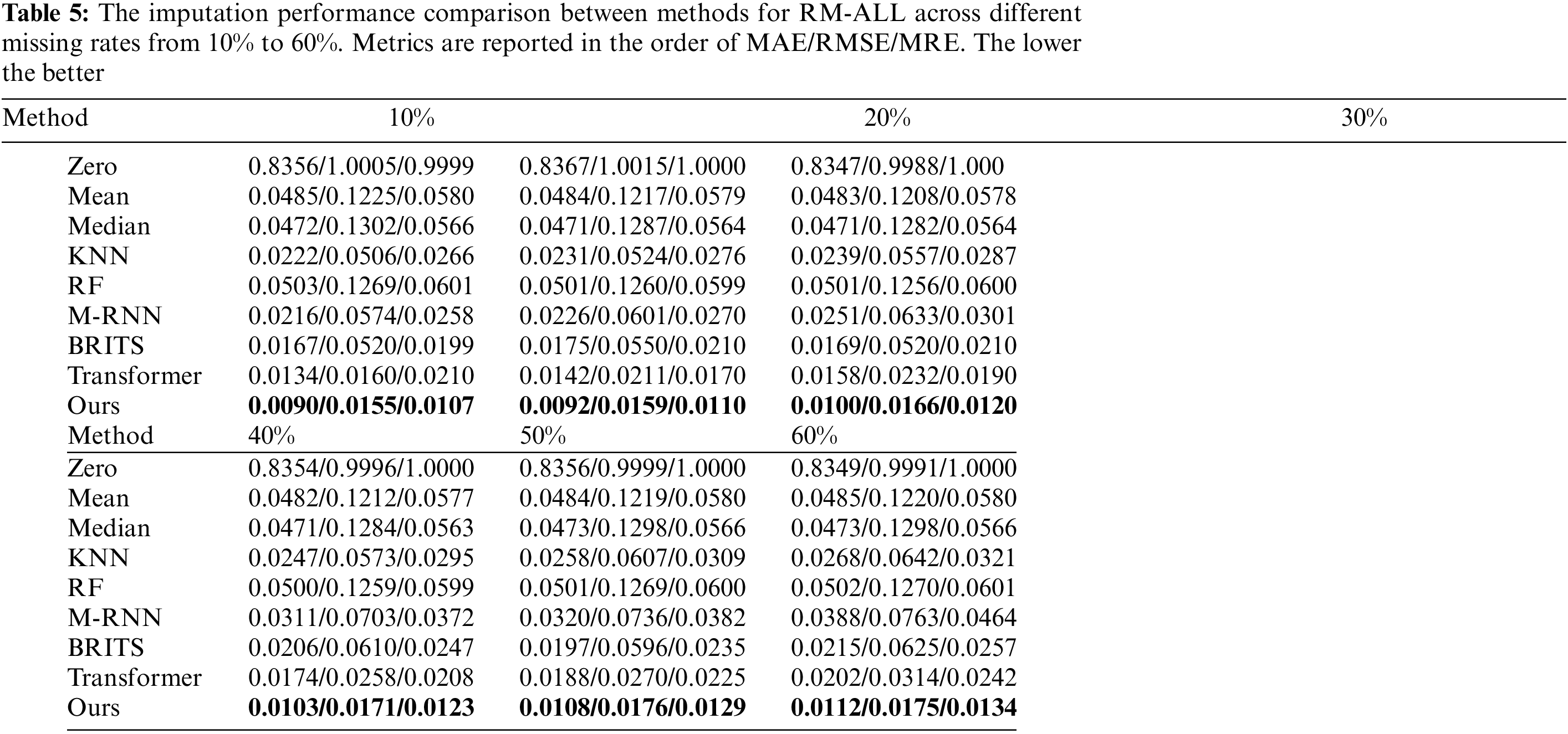
Zero imputation yielded the least favorable results of all the models, with MAE, RMSE, and MRE values of 0.8356, 1.005, and 0.9999, respectively, for a missing rate of 10%. These results strongly indicate a significant data bias. The KNN surpasses the Mean and Median methods across all missing rates since it incorporates the information from the several nearest neighboring samples. The performance of the RF is inferior to that of the Mean and Median methods. This suggests that the imputation mechanism of RF may not be appropriate for addressing the RM-ALL issue.

Furthermore, the models based on deep learning demonstrate remarkable superiority over other methods for all missing rates. Among the diverse deep-learning models, self-attention-based models produce considerably superior outcomes in comparison to their GRNN-based equivalents. At a missing rate of 10%, the Transformer shows a decrease of 22.2%, 65.0%, and 46.2% in MAE, RMSE, and MRE, respectively, compared to the best GRNN-based method BRITS. Similarly, at a missing rate of 60%, the MAE, RMSE, and MRE illustrate a decline of 6%, 49.8%, and 5.8% compared to BRITS. Finally, our proposed model achieves superior results at all missing rates compared to Transformer, and the MAE decreases by 30.8%, 31.9%, 27.5%, 27.5%, 42.6%, and 44.6% for missing rates of 10%, 20%, 30%, 40%, 50% and 60%, respectively. Compared to BRITS, the MAE, RMSE, and MRE decrease by 46.1%, 70.2%, and 46.2%, respectively, at a 10% missing rate, and by 47.9%, 72.0%, and 47.9% at a 60% missing rate. It is worth noting that the RMSE values of BRITS and M-RNN models are significantly higher than the MAE values, which suggests that large errors have occurred at specific missing data points. The MAE and RMSE of our proposed method are much closer. Consequently, it infers that the model proposed seldom causes significant discrepancies for specific missing data points. The case imputation results illustrated in Figs. 7–9 corroborate the analysis.

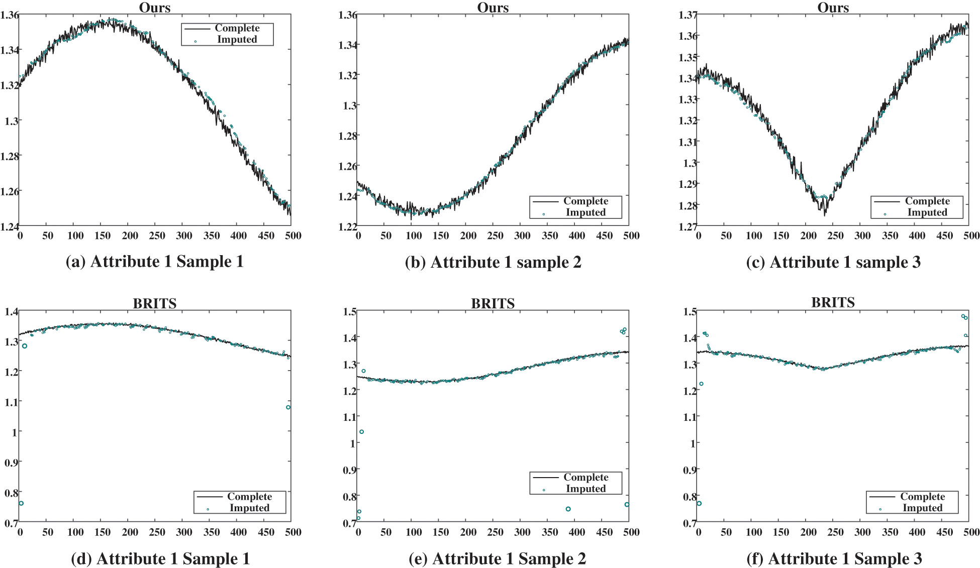
Figure 7: Case imputation results of attribute 1 for missing rate of 40%. (a), (b), and (c) show the imputation results given by our proposed model; (d), (e), and (f) show the results given by BRITS

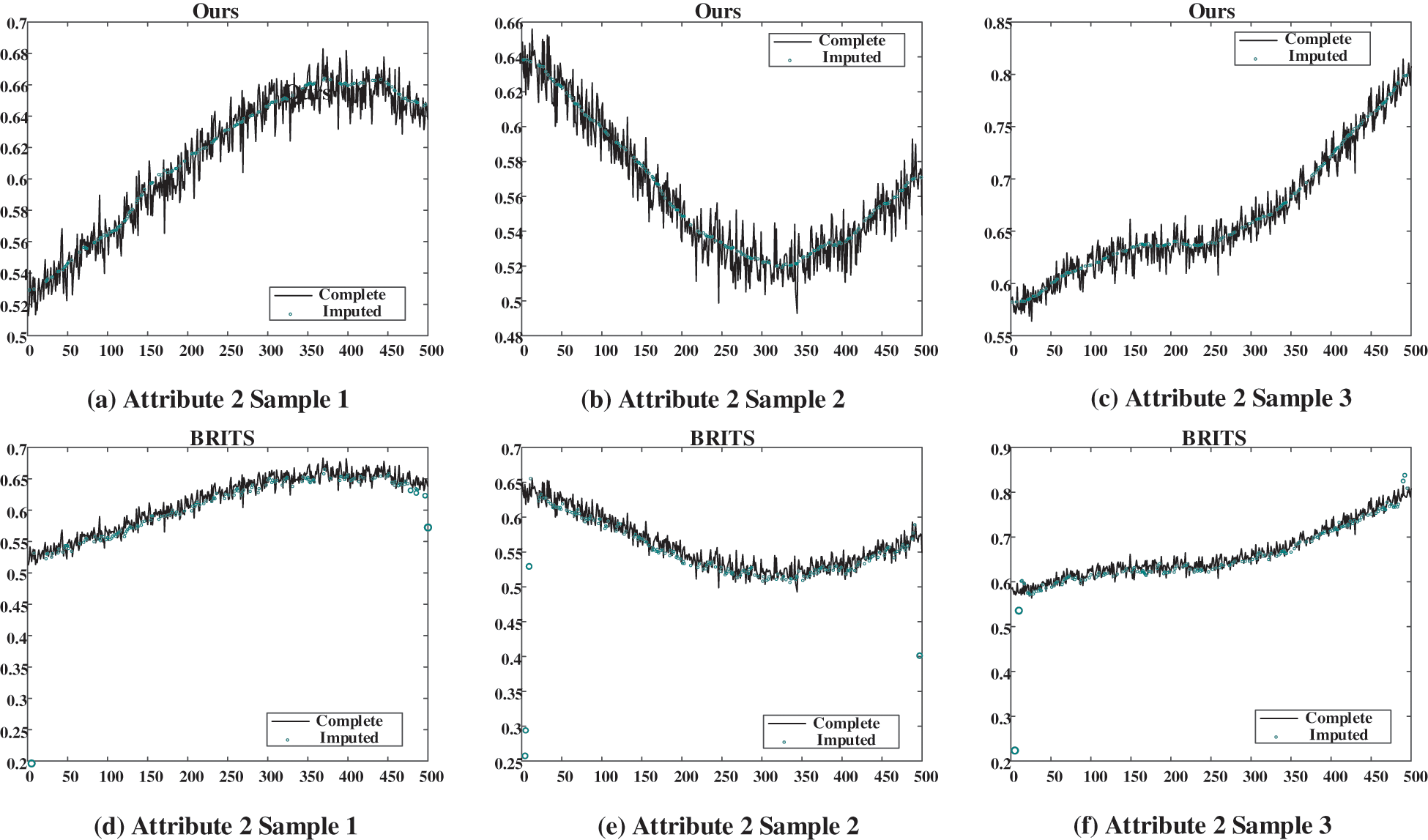
Figure 8: Case imputation results of attribute 2 for missing rate of 40%. (a), (b), and (c) show the imputation results given by our proposed model; (d), (e), and (f) show the results given by BRITS

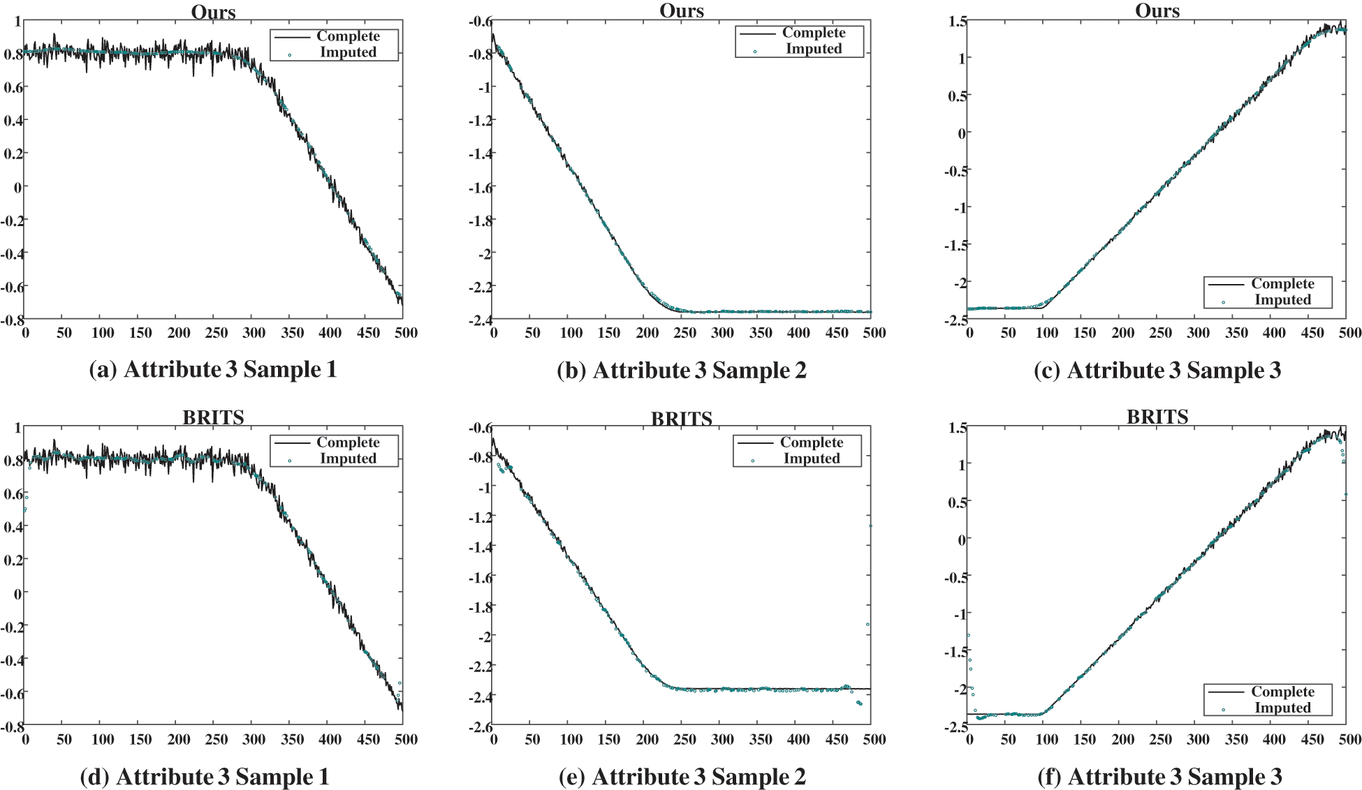
Figure 9: Case imputation results of attribute 3 for the missing rate of 40%. (a), (b), and (c) show the imputation results given by our proposed model; (d), (e), and (f) show the results given by BRITS

In three figures, the imputation results of our proposed model and the BRITS model for three temporally consecutive sliced samples with the missing rate of 40% are presented. The black solid curves represent the ground truth, while the green circles denote the imputed values. It is evident that our proposed model effectively captures the temporal evolution of data and imputes plausible values for the missing data points. Conversely, BRITS’ imputed values for specific missing data points exhibit significant deviations from the actual values, leading to considerable data bias.

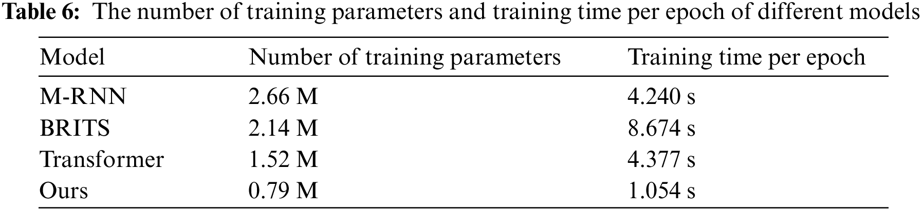
The training parameter count and computational efficiency of various deep learning imputation models in achieving the aforementioned results are examined. The results are listed in Table 6. It is noteworthy that BRITS demonstrates the longest training duration, with a single epoch taking 8.647 s to complete. The M-RNN and Transformer models share similar training times per epoch. Our proposed model showcases fewer training parameters and a shorter training time per epoch than other models. This offers strong evidence supporting its superiority among the considered models.

4.5 Ablation Experiments

In this section, three ablation studies under the RM-ALL scenario are conducted to evaluate the reasonableness of our proposed model. In 4.5.1, the effectiveness of models employing various self-attention mechanisms under different missing rates is assessed and compared; in 4.5.2, the performance of models incorporating different combinations of modules is evaluated and compared; and in 4.5.3, the model’s effectiveness while utilizing different learning objectives is compared.

4.5.1 Ablation Study with Different Self-Attention Mechanisms

Table 7 illustrates the imputation performance of four distinct self-attention mechanisms, applied within our designed identical network structure we designed. The mechanisms are denoted as ‘Full,’ ‘DMSA,’ ‘PSSA,’ and ‘PSDMSA.’ The labels ‘Full,’ ‘DMSA,’ ‘PSSA,’ and ‘PSDMSA’ respectively represent the utilization of vanilla self-attention, diagonal masking self attention, probabilistic sparse self-attention, and probabilistic sparse diagonal masking self attention.

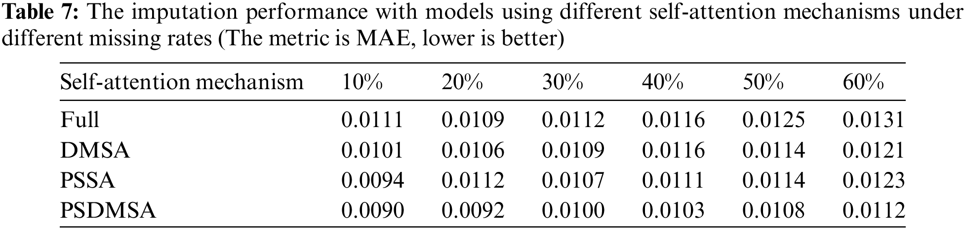
The experimental results demonstrate that the model utilizing PSDMSA consistently outperforms the vanilla self-attention mechanism. Across missing rates of 10%, 20%, 30%, 40%, 50%, and 60%, the MAE values exhibit reductions of 19.0%, 15.6%, 10.7%, 11.2%, 13.6%, and 14.5%, respectively, when using PSDMSA. Additionally, our observations reveal that the model’s performance is enhanced when PSSA and DMSA are jointly utilized, surpassing models that rely exclusively on either mechanism. Specifically, when compared to the DMSA-based model, the PSDMSA-based model achieves MAE reduction rates of 10.9%, 13.2%, 8.3%, 11.2%, 5.3%, and 7.4% at missing rates of 10%, 20%, 30%, 40%, 50%, and 60%, respectively. Moreover, in comparison to the PSSA-based model, the PSDMSA-based model demonstrates MAE reductions of 4.4%, 8.9%, 6.5%, 7.2%, 5.3%, and 8.9% at corresponding missing rates of 10%, 20%, 30%, 40%, 50%, and 60%. These findings collectively suggest that PSDMSA significantly enhances imputation performance.

4.5.2 Ablation Study with Different Combinations of Units

Generally, a more profound network architecture is associated with enhanced feature extraction and knowledge-learning capabilities. Consequently, following the modification of full self-attention and construction of the initial PSDMSA unit, a second unit is incorporated, and the feature vectors learned in the first unit are leveraged for representation reuse. However, the representations derived from the second unit do not consistently surpass those obtained from the first unit. Therefore, it is reasonable to combine the learned representations from both units. To enhance imputation quality, a weight fusion unit that adaptively adjusts the weights of the output representations from both PSDMSA units is introduced.

To prove our design’s better imputation ability, the performance of the four models with different combinations of units are compared in this part. The results are presented in Table 8:

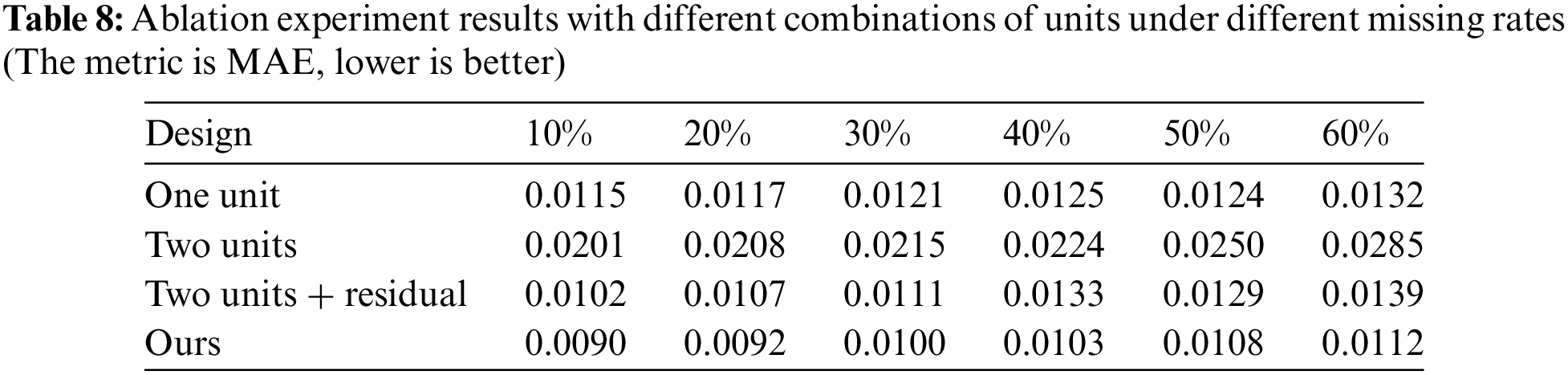
(1) One unit: The second PSDMSA unit and weight fusion unit are not included. The output of only one unit is used as the final representation; (2) Two units: The first and second PSDMSA units are employed without the weight fusion unit, and the output of the second unit is used as the final representation; (3) Two units + residual: The first and second PSDMSA units are employed without the weight fusion unit, and the final representation is derived from the combination of outputs of two units by using a residual connection; (4) Ours.

Based on the experimental findings, it is evident that the imputation performance of the One Unit model is superior to that of the Two Units model. This implies that increasing the network depth does not necessarily lead to improved performance and may even have a detrimental effect. Moreover, when examining the combination of the learned representations from two units, our model, which incorporates the weight fusion unit, outperforms the model that directly combines the outputs of two units using a residual connection (Two units + residual). Additionally, our model achieves better performance than the One-unit model. These findings demonstrate a significant enhancement in imputation performance resulting from our design.

4.5.3 Ablation Study with Different Loss Functions

To evaluate the suitability of imputation loss (IL) for the self-attention-based imputation model and assess its impact on performance enhancement, we compare the imputation performance of our proposed model using IL, reconstruction loss (RL), and a combination of IL + RL as the learning objectives. Eqs.(4) and (27) provide the definition of IL and RL. The results are presented in Table 9.

RL=LOSSMAE(Xoutput3,X,Minput)(27)

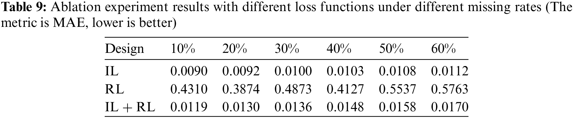
As shown in the table, the PSDMSA-based model’s imputation performance is significantly impaired when RL is applied. This can be attributed to the non-autoregressive nature of the self-attention mechanism, which processes input data globally and in parallel. As a result, observations can be identified through the missing value mask matrix. When RL is used as the loss function, the self-attention-based model minimizes the discrepancy between observed and reconstructed values, neglecting the missing values. Furthermore, the PSDMSA-based model with IL + RL exhibits lower imputation performance than the model employing IL as the learning target. Overall, the model utilizing IL demonstrates optimal imputation performance unaffected by variations in the missing rate. For example, when IL is adopted as the learning objective, the MAE values in a scenario with a 60% missing rate show a decrease of 98.1% and 34.1% compared to models using RL and IL + RL, respectively. This signifies a significant improvement in imputation performance due to the application of IL.

5  Conclusion

This paper proposes a non-autoregressive imputation model that utilizes an improved self-attention mechanism to handle the missing values in RTT-AT. The proposed model consists of two cascaded PSDMSA units incorporating the sparse mechanism, diagonal masking, and a weight fusion unit. The model’s learning objective is to minimize imputation loss.

Initially, two common missing patterns in RTT-AT data are identified and formulated. Next, the differences between the imputed values provided by the proposed model and the other eight models and factual values are analyzed, as demonstrated by MAE, MSE, and MRE. During this process, the missing rates are varied to observe how model performance fluctuates. The experimental results in Sections 4.3 and 4.4 show that our model consistently performs best across both missing patterns, even when the missing rate varies. In the RM-ALT pattern, our model achieves a 31.2%~39.8% reduction in MAE, a 56.2%~58.2% reduction in RMSE, and a 31.2%~39.6% reduction in MRE compared to BRITS, the best GRNN-based imputation model. In the RM-ALL pattern, the reductions are 40.8%~50.0% for MAE, 68.1%~72.0% for RMSE, and 42.9%~50.2% for MRE. Moreover, the MAE and RMSE between imputed values given by our model and their corresponding actual values are much closer, indicating substantially lower bias on specific missing data points and better ability to capture the evolution of the values. Lastly, the parameter counts and training time for multiple models are evaluated. In conclusion, our proposed model stands out as the most cost-effective solution. Compared to BRITS and the vanilla Transformer model, the training time per epoch of our proposed model is just 12.2% and 24.1% of their respective times. In other words, our proposed model accomplishes better imputation performance with less parameter size and time consumption.

Additionally, ablation experiments investigate the impact of attention mechanisms, module combinations, and loss functions on imputation performance. The results show that our model achieves outstanding imputation performance, highlighting the effectiveness of its design choices. Integrating PSDMSA, the weight fusion unit, and imputation loss effectively enhances the model’s imputation performance.

However, our model currently focuses on two missing patterns, RM-ALT and RM-ALL, and does not investigate its performance on other types of missingness, such as long gap missing. Furthermore, the model’s performance in the presence of outliers and noise in the data has not been explored yet. In future work, we will explore the model’s imputation capabilities in extreme scenarios, including long-term missing data and the coexistence of multiple missing patterns. Furthermore, we will utilize the current findings to perform experiments on downstream tasks, specifically classification and prediction, to evaluate the plausibility of the imputation outcomes.

Acknowledgement: The authors are very grateful to the referees and editors for their valuable remarks, which improved the presentation of the paper.

Funding Statement: This work was supported by Graduate Funded Project (No. JY2022A017).

Author Contributions: The authors confirm their contribution to the paper as follows: conception and design: Zihao Song, Yan Zhou, and Futai Liang; manuscript preparation: Zihao Song, Yan Zhou, and Wei Cheng; software: Zihao Song, and Chenhao Zhang; supervision: Yan Zhou, and Wei Cheng. All authors reviewed the results and approved the final version of the manuscript.

Availability of Data and Materials: The data used or analyzed during the current study are available from the corresponding author on reasonable request.

Conflicts of Interest: The authors declare that they have no conflicts of interest to report regarding the present study.

References

1. X. Olive, L. Basora, B. Viry, and R. Alligier, “Deep trajectory clustering with autoencoders,” in ICRAT 2020, 9th Int. Conf. Res. Air Transp., 2020. Accessed: Sep. 18, 2023. [Online]. Available: https://enac.hal.science/hal-02916241 [Google Scholar]

2. X. Pan, Y. He, H. Wang, W. Xiong, and X. Peng, “Mining regular behaviors based on multidimensional trajectories,” Expert Syst. Appl., vol. 66, no. 3, pp. 106–113, Dec. 2016. doi: 10.1016/j.eswa.2016.09.015. [Google Scholar] [CrossRef]

3. M. Gariel, A. N. Srivastava, and E. Feron, “Trajectory clustering and an application to airspace monitoring,” IEEE Trans. Intell. Transp., vol. 12, no. 4, pp. 1511–1524, Dec. 2011. doi: 10.1109/TITS.2011.2160628. [Google Scholar] [CrossRef]

4. Z. Wei, D. Ding, H. Zhou, Z. Zhang, L. Xie, and L. Wang, “A flight maneuver recognition method based on multi-strategy affine canonical time warping,” Appl. Soft Comput., vol. 95, pp. 106527, Oct. 2020. doi: 10.1016/j.asoc.2020.106527. [Google Scholar] [CrossRef]

5. Z. Xi, Y. Lyu, Y. Kou, Z. Li, and Y. Li, “An online ensemble semi-supervised classification framework for air combat target maneuver recognition,” Chinese J. Aeronaut., vol. 36, no. 6, pp. 340–360, Jun. 2023. doi: 10.1016/j.cja.2023.04.020. [Google Scholar] [CrossRef]

6. X. Jing, H. Wang, M. Hou, Y. Liu, and W. Liang, “Study on air combat maneuvering recognition method based on centerline estimation and immune fuzzy neural network,” in L. Yan, H. Duan, X. Yu (Eds.Advances in Guidance, Navigation and Control, Singapore: Springer, 2022, pp. 5109–5120. doi: 10.1007/978-981-15-8155-7_421. [Google Scholar] [CrossRef]

7. Y. Wang, J. Wang, S. Fan, and Y. Wang, “Quick intention identification of an enemy aerial target through information classification processing,” Aerosp. Sci. Technol., vol. 132, no. 19, pp. 108005, Jan. 2023. doi: 10.1016/j.ast.2022.108005. [Google Scholar] [CrossRef]

8. S. Wang, G. Wang, Q. Fu, Y. Song, J. Liu, and S. He, “STABC-IR: An air target intention recognition method based on bidirectional gated recurrent unit and conditional random field with space-time attention mechanism,” Chinese J. Aeronaut., vol. 36, no. 3, pp. 316–334, Nov. 2022. doi: 10.1016/j.cja.2022.11.018. [Google Scholar] [CrossRef]

9. J. Xia, M. Chen, and W. Fang, “Air combat intention recognition with incomplete information based on decision tree and GRU network,” Entropy, vol. 25, no. 4, pp. 671, Apr. 2023. doi: 10.3390/e25040671. [Google Scholar] [PubMed] [CrossRef]

10. M. Gupta, J. Gao, C. C. Aggarwal, and J. Han, “Outlier detection for temporal data: A survey,” IEEE Trans. Knowl. Data Eng., vol. 26, no. 9, pp. 2250–2267, Sep. 2014. doi: 10.1109/TKDE.2013.184. [Google Scholar] [CrossRef]

11. A. B. Batista Júnior, and P. S. da M. Pires, “An approach to outlier detection and smoothing applied to a trajectography radar data,” J. Aerosp. Technol. Manag, vol. 6, no. 3, pp. 237–248, Sep. 2014. doi: 10.5028/jatm.v6i3.325. [Google Scholar] [CrossRef]

12. A. Belhadi, Y. Djenouri, J. C. W. Lin, and A. Cano, “Trajectory outlier detection: Algorithms, taxonomies, evaluation, and open challenges,” ACM Trans. Manage. Inf. Syst., vol. 11, no. 3, pp. 29, Jun. 2020. doi: 10.1145/3399631. [Google Scholar] [CrossRef]

13. Y. Ji, L. Wang, W. Wu, H. Shao, and Y. Feng, “A method for LSTM-based trajectory modeling and abnormal trajectory detection,” IEEE Access, vol. 8, pp. 104063–104073, 2020. doi: 10.1109/ACCESS.2020.2997967. [Google Scholar] [CrossRef]

14. R. Luo, S. Huang, Y. Zhao, and Y. Song, “Threat assessment method of low altitude slow small (LSS) targets based on information entropy and AHP,” Entropy, vol. 23, no. 10, pp. 1292, Oct. 2021. doi: 10.3390/e23101292. [Google Scholar] [PubMed] [CrossRef]

15. X. Chen, X. Wang, H. B. Zhang, Y. H. Xu, Y. Chen and X. T Wu, “Interval TOPSIS with a novel interval number comprehensive weight for threat evaluation on uncertain information,” J. Intell. Fuzzy Syst., vol. 42, no. 4, pp. 4241–4257, Jan. 2022. doi: 10.3233/JIFS-210945. [Google Scholar] [CrossRef]

16. X. Wang, J. Liu, T. Hou, and C. Pan, “The SSA-BP-based potential threat prediction for aerial target considering commander emotion,” Def. Technol., vol. 18, no. 11, pp. 2097–2106, Nov. 2022. doi: 10.1016/j.dt.2021.05.017. [Google Scholar] [CrossRef]

17. S. Ma, H. Zhang, and G. Yang, “Target threat level assessment based on cloud model under fuzzy and uncertain conditions in air combat simulation,” Aerosp. Sci. Technol., vol. 67, no. 6, pp. 49–53, Aug. 2017. doi: 10.1016/j.ast.2017.03.033. [Google Scholar] [CrossRef]

18. Y. Lin, Q. Li, D. Guo, J. Zhang, and C. Zhang, “Tensor completion-based trajectory imputation approach in air traffic control,” Aerosp. Sci. Technol., vol. 114, pp. 106754, Jul. 2021. doi: 10.1016/j.ast.2021.106754. [Google Scholar] [CrossRef]

19. A. Jadhav, D. Pramod, and K. Ramanathan, “Comparison of performance of data imputation methods for numeric dataset,” Appl. Artif. Intell., vol. 33, no. 10, pp. 913–933, Aug. 2019. doi: 10.1080/08839514.2019.1637138. [Google Scholar] [CrossRef]

20. Y. Sun, S. Song, C. Wang, and J. Wang, “Swapping repair for misplaced attribute values,” in 2020 IEEE 36th Int. Conf. Data Eng. (ICDE), Apr. 2020, pp. 721–732. doi: 10.1109/ICDE48307.2020.00068. [Google Scholar] [CrossRef]

21. G. Batista, and M. C. Monard, “A study of k-nearest neighbour as an imputation method,” Presented at the Hybrid break=``Y" Intell. Syst., ser Front Artif. Intell. Appl., Jan. 2002, pp. 251–260. [Google Scholar]

22. X. Jia, X. Dong, M. Chen, and X. Yu, “Missing data imputation for traffic congestion data based on joint matrix factorization,” Knowl-Based Syst., vol. 225, no. 3, pp. 107114, Aug. 2021. doi: 10.1016/j.knosys.2021.107114. [Google Scholar] [CrossRef]

23. P. Zhang, P. Ren, Y. Liu, and H. Sun, “Autoregressive matrix factorization for imputation and forecasting of spatiotemporal structural monitoring time series,” Mech. Syst. Signal Process., vol. 169, no. 12, pp. 108718, Apr. 2022. doi: 10.1016/j.ymssp.2021.108718. [Google Scholar] [CrossRef]

24. W. L. Junger and A. P. de Leon, “Imputation of missing data in time series for air pollutants,” Atmos. Environ., vol. 102, no. 1, pp. 96–104, Feb. 2015. doi: 10.1016/j.atmosenv.2014.11.049. [Google Scholar] [CrossRef]

25. F. V. Nelwamondo, S. Mohamed, and T. Marwala, “Missing data: A comparison of neural network and expectation maximization techniques,” Curr. Sci., vol. 93, no. 11, pp. 1514–1521, 2007. [Google Scholar]

26. S. Song, A. Zhang, J. Wang, and P. S. Yu, “SCREEN: Stream data cleaning under speed constraints,” in Proc. 2015 ACM SIGMOD Int. Conf. Manag. Data, in SIGMOD ‘15, New York, NY, USA: Association for Computing Machinery, May 2015, pp. 827–841. doi: 10.1145/2723372.2723730. [Google Scholar] [CrossRef]

27. S. Song, A. Zhang, L. Chen, and J. Wang, “Enriching data imputation with extensive similarity neighbors,” Proc. VLDB Endow., vol. 8, no. 11, pp. 1286–1297, Jul. 2015. doi: 10.14778/2809974.2809989. [Google Scholar] [CrossRef]

28. K. He, X. Zhang, S. Ren, and J. Sun, “Deep residual learning for image recognition,” in IEEE Conf. Comput. Vis. Pattern Recogn., 2016. Accessed: May 08, 2023. [Online]. Available: https://www.zhangqiaokeyan.com/academic-conference-foreign_meeting_thesis/0705015997307.html [Google Scholar]

29. J. Devlin, M. W. Chang, K. Lee, and K. Toutanova, “BERT: Pre-training of deep bidirectional transformers for language understanding,” arXiv:1810.04805 2019. doi: 10.48550/arXiv.1810.04805. [Google Scholar] [CrossRef]

30. W. Bao, Y. Gu, B. Chen, and H. Yu, “Golgi_DF: Golgi proteins classification with deep forest,” Front. Neurosci., vol. 17, pp. 106, Nov. 2023 doi: 10.3389/fnins.2023.1197824. [Google Scholar] [PubMed] [CrossRef]

31. W. Bao, B. Yang, D. Li, Z. Li, Y. Zhou and R. Bao, “CMSENN: Computational modification sites with ensemble neural network,” Chemometr. Intell. Lab. Syst., vol. 185, no. 5507, pp. 65–72, Feb. 2019. doi: 10.1016/j.chemolab.2018.12.009. [Google Scholar] [CrossRef]

32. P. B. Weerakody, K. W. Wong, G. Wang, and W. Ela, “A review of irregular time series data handling with gated recurrent neural networks,” Neurocomput., vol. 441, no. 7, pp. 161–178, Jun. 2021. doi: 10.1016/j.neucom.2021.02.046. [Google Scholar] [CrossRef]

33. H. Yuan, G. Xu, Z. Yao, J. Jia, and Y. Zhang, “Imputation of missing data in time series for air pollutants using long short-term memory recurrent neural networks,” in Proc. 2018 ACM Int. Joint Conf. 2018 Int. Symp. Pervas. Ubiquitous Comput. Wearable Comput., in UbiComp ‘18, New York, NY, USA: Association for Computing Machinery, Oct. 2018, pp. 1293–1300. doi: 10.1145/3267305.3274648. [Google Scholar] [CrossRef]

34. J. Zhang, X. Mu, J. Fang, and Y. Yang, “Time series imputation via integration of revealed information based on the residual shortcut connection,” IEEE Access, vol. 7, pp. 102397–102405, 2019. doi: 10.1109/ACCESS.2019.2928641. [Google Scholar] [CrossRef]

35. J. Yoon, W. R. Zame, and M. van der Schaar, “Estimating missing data in temporal data streams using multi-directional recurrent neural networks,” IEEE Trans. Biomed. Eng., vol. 66, no. 5, pp. 1477–1490, May 2019. doi: 10.1109/TBME.2018.2874712. [Google Scholar] [PubMed] [CrossRef]

36. W. Cao, D. Wang, J. Li, H. Zhou, L. Li and Y. Li, “BRITS: Bidirectional recurrent imputation for time series,” in Adv. Neur. Inf. Process. Syst., Curran Assoc., Inc., 2018. Accessed: Sep. 21, 2023. [Online]. Available: https://proceedings.neurips.cc/paper_files/paper/2018/hash/734e6bfcd358e25ac1db0a4241b95651-Abstract.html [Google Scholar]

37. J. Brittain, M. Cendon, J. Nizzi, and J. Pleis, “Data scientist’s analysis toolbox: Comparison of python, R, and SAS performance,” SMU Data Sci. Rev., vol. 1, no. 2, Jul. 2018. https://scholar.smu.edu/datasciencereview/vol1/iss2/7 [Google Scholar]

38. C. F. Tsai and Y. H. Hu, “Empirical comparison of supervised learning techniques for missing value imputation,” Knowl. Inf. Syst., vol. 64, no. 4, pp. 1047–1075, Apr. 2022. doi: 10.1007/s10115-022-01661-0. [Google Scholar] [CrossRef]

39. I. Pratama, A. E. Permanasari, I. Ardiyanto, and R. Indrayani, “A review of missing values handling methods on time-series data,” in Int. Conf. Inf. Technol. Syst. Innov. (ICITSI), Oct. 2016, pp. 1–6. doi: 10.1109/ICITSI.2016.7858189. [Google Scholar] [CrossRef]

40. D. Fung, “Methods for the estimation of missing values in time series,” Theses: Doctorates and Masters,” 2006 Accessed: Jan. 3, 2024. [Online]. Available: https://ro.ecu.edu.au/theses/63 [Google Scholar]

41. X. Chen, M. Lei, N. Saunier, and L. Sun, “Low-rank autoregressive tensor completion for spatiotemporal traffic data imputation,” IEEE Trans. Intell. Transport. Syst., vol. 23, no. 8, pp. 12301–12310, Aug. 2022. doi: 10.1109/TITS.2021.3113608. [Google Scholar] [CrossRef]

42. M. Amiri and R. Jensen, “Missing data imputation using fuzzy-rough methods,” Neurocomput., vol. 205, pp. 152–164, Sep. 2016. doi: 10.1016/j.neucom.2016.04.015. [Google Scholar] [CrossRef]

43. N. A. A. Wafaa Mustafa Hameed, “Comparison of seventeen missing value imputation techniques,” J. Hunan Univ, Natur. Sci., vol. 49, no. 7, 2022. Accessed: Dec. 26, 2023. [Online]. Available:. http://jonuns.com/index.php/journal/article/view/1113 [Google Scholar]

44. S. Song, L. Chen, and H. Cheng, “Efficient determination of distance thresholds for differential dependencies,” IEEE Trans. Knowl. Data Eng., vol. 26, no. 9, pp. 2179–2192, Sep. 2014. doi: 10.1109/TKDE.2013.84. [Google Scholar] [CrossRef]

45. S. Song, L. Chen, and P. S. Yu, “Comparable dependencies over heterogeneous data,” The VLDB J., vol. 22, no. 2, pp. 253–274, Apr. 2013. doi: 10.1007/s00778-012-0285-7. [Google Scholar] [CrossRef]

46. J. Wang, S. Song, X. Lin, X. Zhu, and J. Pei, “Cleaning structured event logs: A graph repair approach,” in 2015 IEEE 31st Int. Conf. Data Eng., Apr. 2015, pp. 30–41. doi: 10.1109/ICDE.2015.7113270. [Google Scholar] [CrossRef]

47. C. Fang, and C. Wang, “Time series data imputation: A survey on deep learning approaches,” arXiv:2011.11347, 2020. doi: 10.48550/arXiv.2011.11347. [Google Scholar] [CrossRef]

48. Md G. Rahman and M. Z. Islam, “Missing value imputation using decision trees and decision forests by splitting and merging records: Two novel techniques,” Knowl.-Based Syst., vol. 53, no. 1, pp. 51–65, Nov. 2013. doi: 10.1016/j.knosys.2013.08.023. [Google Scholar] [CrossRef]

49. E. L. Silva-Ramírez, R. Pino-Mejías, and M. López-Coello, “Single imputation with multilayer perceptron and multiple imputation combining multilayer perceptron and k-nearest neighbours for monotone patterns,” Appl. Soft Comput., vol. 29, no. 7A, pp. 65–74, Apr. 2015. doi: 10.1016/j.asoc.2014.09.052. [Google Scholar] [CrossRef]

50. F. Tang, and H. Ishwaran, “Random forest missing data algorithms, statistical analysis and data mining: The ASA,” Data Sci. J., vol. 10, no. 6, pp. 363–377, 2017. doi: 10.1002/sam.11348. [Google Scholar] [PubMed] [CrossRef]

51. Q. Ni, and X. Cao, “MBGAN: An improved generative adversarial network with multi-head self-attention and bidirectional RNN for time series imputation,” Eng. Appl. Artif. Intell., vol. 115, no. 1, pp. 105232, Oct. 2022. doi: 10.1016/j.engappai.2022.105232. [Google Scholar] [CrossRef]

52. Y. Luo, X. Cai, Y. Zhang, J. Xu, and X. J. Yuan, “Multivariate time series imputation with generative adversarial networks,” in Adv. Neur. Inf. Process. Syst., Curran Assoc., Inc., 2018. Accessed: Dec. 29, 2023. [Online]. Available: https://proceedings.neurips.cc/paper_files/paper/2018/hash/96b9bff013acedfb1d140579e2fbeb63-Abstract.html [Google Scholar]

53. Z. Wu et al., “BRNN-GAN: Generative adversarial networks with bi-directional recurrent neural networks for multivariate time series imputation,” in 2021 IEEE 27th Int. Conf. Parallel and Distrib. Syst. (ICPADS), Dec. 2021, pp. 217–224. doi: 10.1109/ICPADS53394.2021.00033. [Google Scholar] [CrossRef]

54. T. Salimans et al., “Improved techniques for training GANs,” in Adv. Neur. Inf. Process. Syst., Curran Assoc., Inc., 2016. Accessed: Dec. 29, 2023. [Online], Available: https://proceedings.neurips.cc/paper_files/paper/2016/hash/8a3363abe792db2d8761d6403605aeb7-Abstract.html [Google Scholar]

55. A. Vaswani et al., “Attention is all you need,” in I. Guyon, U. V. Luxburg, S. Bengio, H. Wallach, R. Fergus, S. Vishwanathan (Eds.Advances in Neural Information Processing Systems 30 (NIPS 2017), 2017. Accessed: Apr. 12, 2023. [Online]. Available: https://www.webofscience.com/wos/alldb/full-record/WOS:000452649406008 [Google Scholar]

56. H. Zhou et al., “Informer: Beyond efficient transformer for long sequence time-series forecasting,” arXiv:2012.07436, 2021. doi: 10.48550/arXiv.2012.07436. [Google Scholar] [CrossRef]

57. A. W. C. Liew, N. F. Law, and H. Yan, “Missing value imputation for gene expression data: Computational techniques to recover missing data from available information,” Brief. Bioinf., vol. 12, no. 5, pp. 498–513, Sep. 2011. doi: 10.1093/bib/bbq080. [Google Scholar] [PubMed] [CrossRef]