PAV-A-kNN: A Novel Approachable kNN Query Method in Road Network Environments

1  Introduction

The rapid advancement of mobile communication and spatial positioning technologies has led to the widespread adoption of Location-Based Services (LBS), fueling the swift development of user-centric urban transportation systems. LBS applications are especially prominent in road network environments. For instance, in navigation systems like Gaode Map, users may seek the shortest path between two locations. Meanwhile, in LBS applications such as DiDi or cargo transport platforms like Huolala, users issue requests based on their current location. In these cases, the system needs to select the k nearest vehicles to the user for scheduling to fulfill their needs. These application scenarios necessitate efficient spatial object queries within road networks, such as k-nearest neighbor (kNN) searches. Therefore, developing methods to efficiently handle such location-based spatial queries in road networks is of significant importance. A substantial amount of research [1–3] has been conducted on the query problem of moving objects in road networks. However, many of these studies assume that all moving objects can immediately respond to user requests upon receiving a query. In practice scenarios, this assumption is not always valid. On one hand, due to high user demand, vehicles near the query point may already be occupied and unable to respond to new requests. On the other hand, vehicles that are currently performing tasks may become potential candidates for the query once they reach their destinations, especially if their destinations are close to the query point. Thus, a class of queries known as Approachable-kNN (A-kNN) [4] has been proposed in the industry. The objective of A-kNN is to return the top k moving objects that can respond to a query request at the earliest after completing their current tasks, given a query point Q and a set of moving objects M. Therefore, the distance metric between the query point and a moving object is redefined as the sum of the remaining distance to the object’s destination and the distance from that destination to the query point. However, with the rapid growth of travel demand and the increasing complexity of road network structures, computing the shortest distance between arbitrary vertex pairs has become time-consuming. If the shortest distances between vertices can be precomputed and stored in advance, query processing costs can be significantly reduced, thereby improving overall query efficiency. Based on this idea, researchers have proposed tree-based index structures such as V-Tree [5] to efficiently support kNN queries for moving objects in road networks. However, most existing methods tend to overlook semantic constraints, particularly the involvement of moving objects (e.g., drivers) in ongoing tasks with specific destinations, which may lead to suboptimal scheduling outcomes in real-world applications. In large ride-hailing platforms like Didi or Uber, when a customer submits a request, the system must identify the earliest-responding driver among thousands of candidates. Traditional methods such as V-Tree and G-Tree consider only spatial proximity, neglecting the fact that some drivers are currently en route to their respective destinations. As illustrated in Fig. 1, O3 is identified as closest to the query point Q based on its current location. Consequently, O3 may be mistakenly selected as the nearest driver for the query request. However, since O3 is en route to its destination D3, which is far from the Q, it is not the most appropriate choice. In contrast, O2—though spatially farther—has a shorter aggregate distance (i.e., the remaining distance to its destination plus the distance from that destination to Q), making it a more suitable candidate. Such misjudgments may lead to service delays and a suboptimal user experience, clearly highlighting the importance of incorporating destination-aware semantic constraints in spatial query processing.

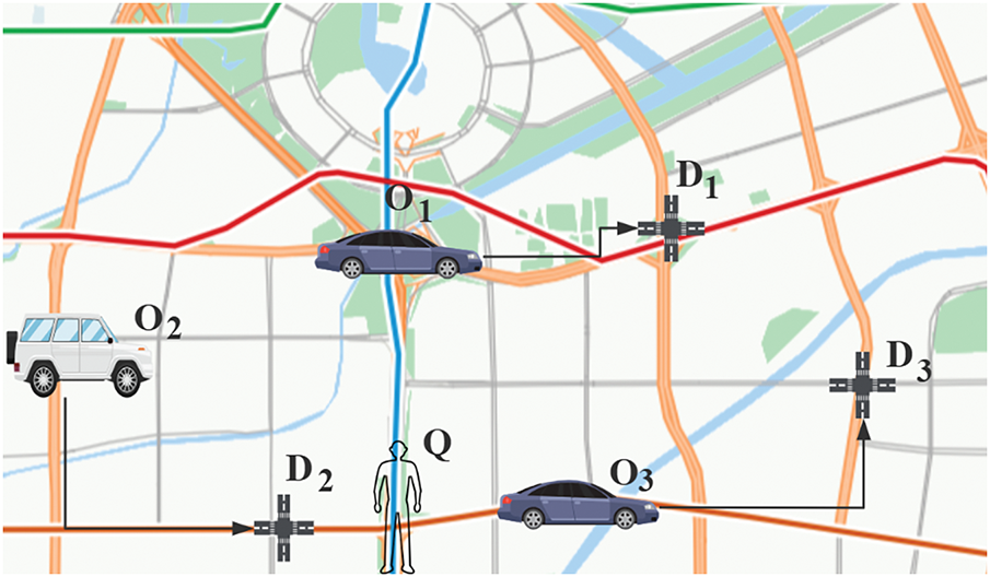
Figure 1: An example of A-kNN query

In addition, when two query vertices are close in the actual road network but assigned to farther leaf nodes in the V-Tree, the query process may require traversing numerous irrelevant subgraphs and their boundary vertices until reaching the optimal solution. For instance, as shown in the road network of Fig. 2a, when computing the shortest distance between vertices v12 and v6, the V-Tree-based query method needs to access the boundary vertices of four nodes: D, A, B, and E, to obtain the solution. To address this issue, this paper proposes an improved indexing structure based on V-Tree called the Path-Accelerated V-Tree (PAV-Tree). To accelerate distance queries, PAV-Tree constructs shortcuts between designed leaf nodes, where each shortcut records the shortest path distances among all boundary vertices within the two nodes. For example, as illustrated in Fig. 2b, two shortcuts, S1 and S2, respectively connect leaf nodes C − F and D − E. Consequently, calculating the distance between vertices v12 and v6 only requires accessing the shortcut S2 and the distance matrix of node E, which is significantly more efficient than the V-Tree approach. Based on our experiments on real-world road network datasets, the proposed method is particularly well-suited for large-scale ride-hailing platforms, where high-frequency spatiotemporal queries over millions of moving objects are routine. By reducing unnecessary candidate evaluations and employing pruning strategies, the method significantly improves query efficiency. Compared with traditional approaches, our solution achieves over a 45% reduction in query processing time, leading to substantial savings in computational resources. Furthermore, the reduction in scheduling latency directly enhances user experience and driver utilization, offering both operational and economic benefits for commercial platforms. The key contributions of this paper can be summarized as follows:

1.    We propose a novel index, PAV-Tree, which is better than the V-Tree in handling road network-based A-kNN queries.

2.    Building on PAV-Tree, we introduce a shortcut-based algorithm, PAV-A-kNN, to answer A-kNN queries, demonstrating greater efficiency than the V-Tree-based algorithm.

3.    Extensive experiments on real-world and synthetic datasets indicate that the query performance based on method PAV-A-kNN is significantly better than that based on V-Tree-based kNN in road networks.

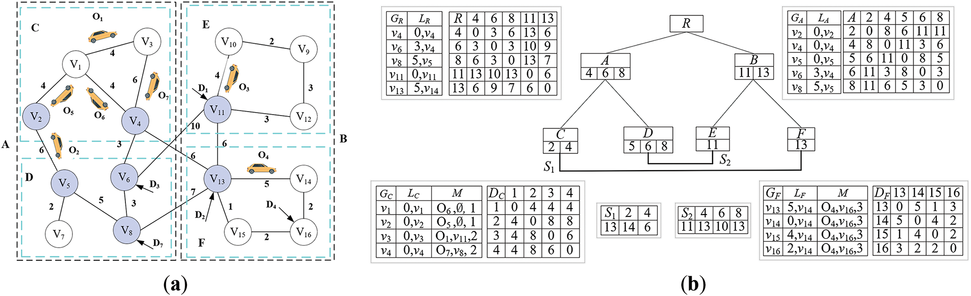
Figure 2: An example of PAV-Tree index (f = 2, τ = 4). Matrices of some nodes are omitted. (a) Graph partition. (b) PAV-Tree

2  Related Work

Road network-based kNN queries have been a hot research topic [6–9]. The most basic solution to the kNN query problem is the Dijkstra algorithm [10]. Given a query point q, the algorithm iteratively explores vertices in increasing order of distance util k nearest objects are found. While effective, this approach becomes computationally expensive, particularly in large-scale networks. To address these challenges, researchers have developed index structures and algorithms that precompute and store critical information, significantly enhancing query efficiency in large road networks. Notable index-based query methods include G-Tree [11], and V-Tree [5].

G-Tree partitions the whole graph into subgraphs, utilizes a balanced tree structure to maintain these subgraphs, and uses an assembly-based approach to answer kNN queries. G*-Tree [12] overcomes this drawback by creating shortcuts between selected leaf nodes. However, when there are no shortcuts between leaf nodes, G*-Tree still requires significant computational cost and time to traverse its subtrees. V-Tree inherits G-Tree, identifying boundary vertices of subgraphs and employing efficient techniques to process kNN queries by maintaining a list of objects near the boundary vertices.

Li et al. [13] developed a method to address the challenge of continuously reporting alternative paths for users traveling along a specified route by sequentially accessing vertices in increasing order of maximum depth values. This approach improves both computational efficiency and accuracy. To extend kNN queries to multiple moving objects, Abeywickrama et al. [14] introduced the Compressed Object Landmark Tree (COLT) structure, which facilitates efficient hierarchical graph traversal and supports various aggregation functions.

In recent years, researchers have provided new solutions for kNN queries in terms of optimizing throughput including TOAIN [15] and GLAD [16]. TOAIN uses SCOB indexing and contraction hierarchy (CH) [17] structure, which creates shortcuts within the graph. These shortcuts enable the pre-computation of candidate downhill objects before performing the kNN-Dijkstra search, thereby improving efficiency. Additionally, TOAIN conducts a workload analysis to configure the SCOB indexing, ensuring maximum throughput. GLAD, by comparison, uses an index of the grid to store moving objects, divides the road network into 2x⋅2x grids based on vertex latitude and longitude, and maintains lists containing objects for each grid, and it employs a jump-tag based structure H2H [18] to compute the distance between vertices. Since the update cost of the grid is low, GLAD can realize a small update cost, thus improving the throughput of the system.

A relatively advanced approach is the tree decomposition kNN [19] search algorithm, which employs a tree-based partitioning method to associate each vertex with a corresponding node in the tree. This approach efficiently calculates the shortest path between nodes. However, it necessitates recalculating the inputs for updated k-values, which results in greater time overhead due to redundant computations. In the latest research progress, Wang et al. proposed a concise kNN indexing structure, KNN-Index [20], designed to address the complexity of indexing, high space overhead, and prolonged query latency associated with traditional methods. This method simplifies the index design by directly recording the first k nearest neighbors of each vertex to significantly reduce the index space occupation while supporting progressive optimal query processing.

The shortest path query is a crucial component of kNN queries, particularly for single-pair shortest paths [21–25]. H2H and P2H [26] construct hierarchical labels based on tree decomposition. P2H improves on H2H by pruning certain labels and adding shortcuts between others, achieving optimal performance in a recent experiment [27]. Dan et al. introduced [28] LG-Tree, which divides the entire graph into multiple subgraphs and indexes these subgraphs using a balanced tree. By incorporating Dynamic Index Filtering (DIF) and boundary vertices, combined with phased dynamic programming, to ensure efficient shortest distance queries.

Recently, employing machine learning methods has emerged as a novel research approach to solving shortest distance computation problems. Huang et al. [29] proposed a road network embedding method (RNE) that approximates the shortest path through L1 distance in a low dimensional vector space, achieving nanosecond level query response. However, this method has large errors on long-distance paths and high training costs, and the pruning effect of kNN is affected by high-dimensional features, resulting in a decrease in accuracy.

Zheng et al. proposed RLTD [30], which applies reinforcement learning to optimize tree decomposition for compressing the space overhead of 2-hop label indexing. Although it reduces index size, the method requires costly training, lacks adaptability to dynamic network changes, and offers limited improvements in query performance. Moreover, the learned strategies generalize poorly across different networks.

Drakakis et al. [31] proposed the Neural Bellman Ford Network (NBFN), which combines the classical Bellman-Ford algorithm with Graph Neural Networks (GNNs) through a message-passing mechanism (MPNN) to solve the shortest path problem. While innovative, this approach heavily depends on training data, exhibits large errors on unseen nodes or long paths, suffers from numerical instability, and incurs high computational overhead in sparsely connected networks.

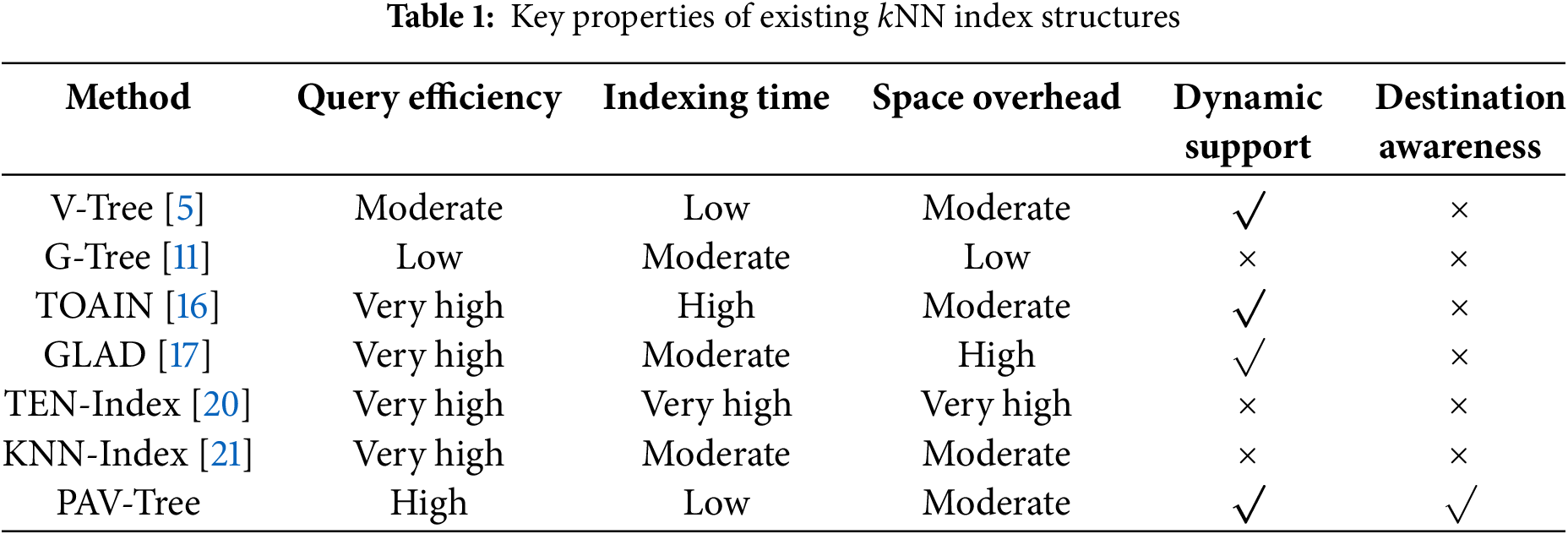
In summary, although these learning-based approaches offer advantages in static scenarios—such as fast querying, index compression, and algorithmic innovation—they face shared challenges: high training cost, limited generalization, and lack of result controllability. In contrast, the PAV-Tree method proposed in this paper, grounded in traditional index structures, features clear organization, no training requirement, and transparent path computation logic, making it well-suited for scenarios demanding high controllability and deployment stability. Table 1 summarizes the key characteristics of existing kNN index structures.

3  Preliminaries

Shortest Path. Given an undirected weighted graph G=(V,E) where V is the set of vertices and E is the set of edges, each edge (u, v) ∈ E has an associated weight representing the distance between u and v. A path from u to v is defined as a sequence of vertices P = ⟨v0, v1, … , vn⟩ where v0 = u and vn = v. The path distance denoted as Path (u, v), is the sum of the weights of all edges in P. The shortest path, denoted as SPath (u, v), is the path with the minimum total distance among all possible paths between the u and v, and the corresponding distance is denoted as SPath(u, v).

For example, in Fig. 3, there are two paths from the vertex v2 to vertex v5, namely v2→v3→v5 and v2→v4→v5. Clearly, SPDist (v2, v5) = 110.

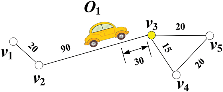
Figure 3: An example of a moving object

Moving Object. Each moving object O is represented as a tuple O=(C,D,S), where C denotes the current position, D denotes the destination of the moving object, and S indicates the status specifying whether the object is occupied. If D = ∅, it indicates that the destination is its active vertex.

Active Vertice. Given an object O on an edge e which is moving to the vertex v, we call O an active object of vertex v and call v an active vertex.

For example, in Fig. 3, the moving object O1 is traveling from vertex v2 to vertex v3 along edge (v2, v3). Thus, O1 is the active object of the active vertex v3, with an offset of 30.

Local Nearest Active Vertex (LNAV) and Global Nearest Active Vertex (GNAV). Given a vertex u in a subgraph Gi, an active vertex v in Gi is called the LNAV of u if the distance from v to u is the smallest among all active vertices in Gi. If the distance from u′ to v is the smallest among all active vertices in the entire graph G, u′ is termed the GNAV of v.

For example, in Fig. 2a, there are seven active vertices. In the subgraph GD, the LNAV of v6 is v5, and in GA, the LNAV of v6 is v4. Meanwhile, the GNAV of v6 is v4.

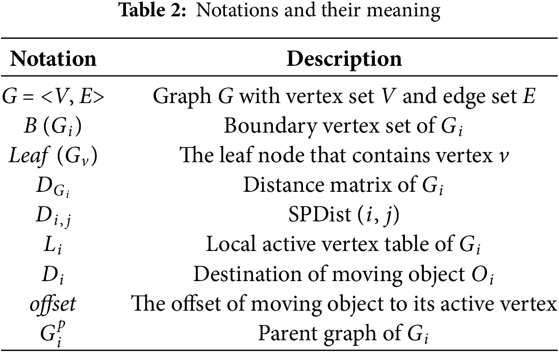
Table 2 provides a summary of the key notations and their corresponding meanings used in this paper.

Boundary vertices. Given a subgraph Gi of a graph G = <V,E> with a vertex β ∈ Gi, β is called a boundary vertex if ∃ (β, v) ∈ E and v ∉ Gi. The set of boundary vertices of Gi is denoted as B (Gi).

A-kNN Query. Given a directed weighted graph G (V, E), a set M of moving objects, an integer k ≤ |M|, an A-kNN query is denoted as A-kNN = (q, k), where q represents the query position. The A-kNN query returns a result set R ⊆ M of k moving objects such that for every O′ ∈ M∖R, the following inequation holds for all O ∈ R.

SPDist(O′.C,O′.D)+SPDist(O′.D,q)≥SPDist(O.C,O.D)+SPDist(O.D,q)

4  The PAV-Tree Index

4.1 Definition of PAV-Tree

A PAV-Tree for a road network G is a balanced search tree that follows a hierarchy of graph partitions and satisfies the following properties:

1.    Each non-leaf node has f children (f≥ 2). Each leaf node contains at most τ vertices (τ ≥ 1).

2.    Each node maintains an LNAV Table L. The leaf nodes store the LNAV for all vertices within the leaf, while the non-leaf nodes store the LNAV of the boundary vertices of all their child nodes.

3.    Each leaf node holds an active object table M, which records the active objects associated with each vertex in the leaf node.

4.    The total size of all shortcuts is at most η (η≥ 0).

In a PAV-Tree, each node corresponds to a subgraph, and vice versa; thus, nodes and subgraphs can be used interchangeably for simplicity.

Example 1. Fig. 2b shows the PAV-Tree of the road network and moving objects in Fig. 2a with f = 2, τ = 4, and η = 5. The shortcuts S1 and S2 store 2 and 3 distance values respectively in the distance matrix. Thus, the shortcut threshold η is 5.

4.2 Data Structure of PAV-Tree

LNAV Table L. Each non-leaf graph Gi stores the LNAV of the boundary vertices of all its child nodes. For a leaf node, L stores the LNAV of all its vertices, denoted by Lx has two columns, LX[β].γ and LX[β].δ, which record β′s LNAV in a node X and β′s distance to its LNAV, respectively.

For example, in Fig. 2a, LD[β].γ=v5, and LD[β].δ = 8.

Active Object Table M. Each leaf node Gi maintains an active object table Mi, where Mi[v] records the active objects associated with vertex v. Each entry in Mi[v] is represented as (O, D, δ), where O is the active object, D is its destination, and δ is its offset from the active vertex.

Space Complexity of PAV-Tree. Given a PAV-Tree with V vertices, M moving objects, and a shortcut threshold η, the space complexity is O(|M|+log⁡|V|+η).

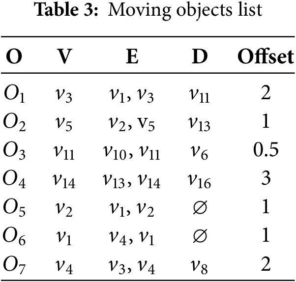
Table 3 records the relevant information of all moving objects in Fig. 2a.

4.3 Shortcut Selection

In this section, we will introduce the method for establishing shortcuts in the PAV tree. Before discussing the creation of shortcuts between leaf nodes, we first need to clarify that the goal of this paper is to build shortcuts between leaf nodes that are geographically close in the graph but distant in the PAV-Tree structure (as explained in Section 1). To achieve this, Definitions 1 and 2 are introduced to determine whether two nodes meet the specified criteria.

Definition 1 (Adjacent cousin nodes). Given leaf nodes Gi and Gj, where u ∈ B (Gi) and v ∈ B (Gj), Gi and are called adjacent cousin nodes, denoted as Gi∼ Gj, if ∃ (u,v) ∈ E and Gi and Gj are cousin nodes.

Furthermore, two nodes are cousins of each other if they are at the same level but have different parent nodes. If two nodes are adjacent cousin nodes, this paper considers them to be geographically close in the graph. Such adjacency indicates that the two nodes are directly connected in the graph while belonging to different subgraphs at the same hierarchical level, reflecting their geographical closeness.

Definition 2. The function Y of two leaf nodes Gi and Gj in PAV-Tree is denoted as:

Y(Gi,Gj)=|B(Gi)|+|B(Gj)|+∑⟨Nx,Ny⟩∈Pi,j|B(Gx)|⋅|B(Gy)|(1)

where pi,j denotes the shortest common ancestor path between leaf nodes Gi and Gj in PAV-Tree. In addition, Nx and Ny represent two consecutive nodes along pi,j.

Based on the time complexity analysis of the G-Tree method [11], the cost of calculating the distance between any two vertices can be assessed by the number of boundary vertices on the shortest common ancestor path between the two vertices. Therefore, a larger value of Y indicates that the algorithm needs to scan more boundary vertices to compute the distance between the two leaf nodes, and thus we consider two leaf nodes in the PAV tree to be “distant.”

Definition 3 (Shortest Common Ancestral Path). Given a subgraph Gi = (Vi, Ei), for two vertices vi ∈ Gi and vj ∈ Gj, the path from vi to vj that traverses their least common ancestor is referred to as the shortest common ancestral path (SCAP). The SCAP between any two vertices is denoted as SCAP (vi, vj) ={Gi→Gi+1⋅⋅⋅→Gj}, where the intermediate subgraphs represent the sequence of subgraph partitions from Gi to Gj. (excluding the least common ancestor).

For example, in Fig. 2a, the SCAP (C, F) is {C, A, B, F}, and SCAP (C, D) is {C, A, D}.

Definition 4 (Shortcut Selection Problem). Let xi,j ∈ {0,1} be an indicator, where xi,j = 1 (or 0) indicates whether a shortcut is selected (or not selected) between the leaf nodes Gi and Gj in the PAV-Tree. Then, the problem of shortcut selection is defined as follows:

∑1≤i,j≤zY(Gi,Gj)⋅xi,j(2)

∑1≤i,j≤z|B(Gi)|⋅|B(Gj)|⋅xi,j≤η(3)

Maximize Eq. (2) under the constraints of Eq. (3).

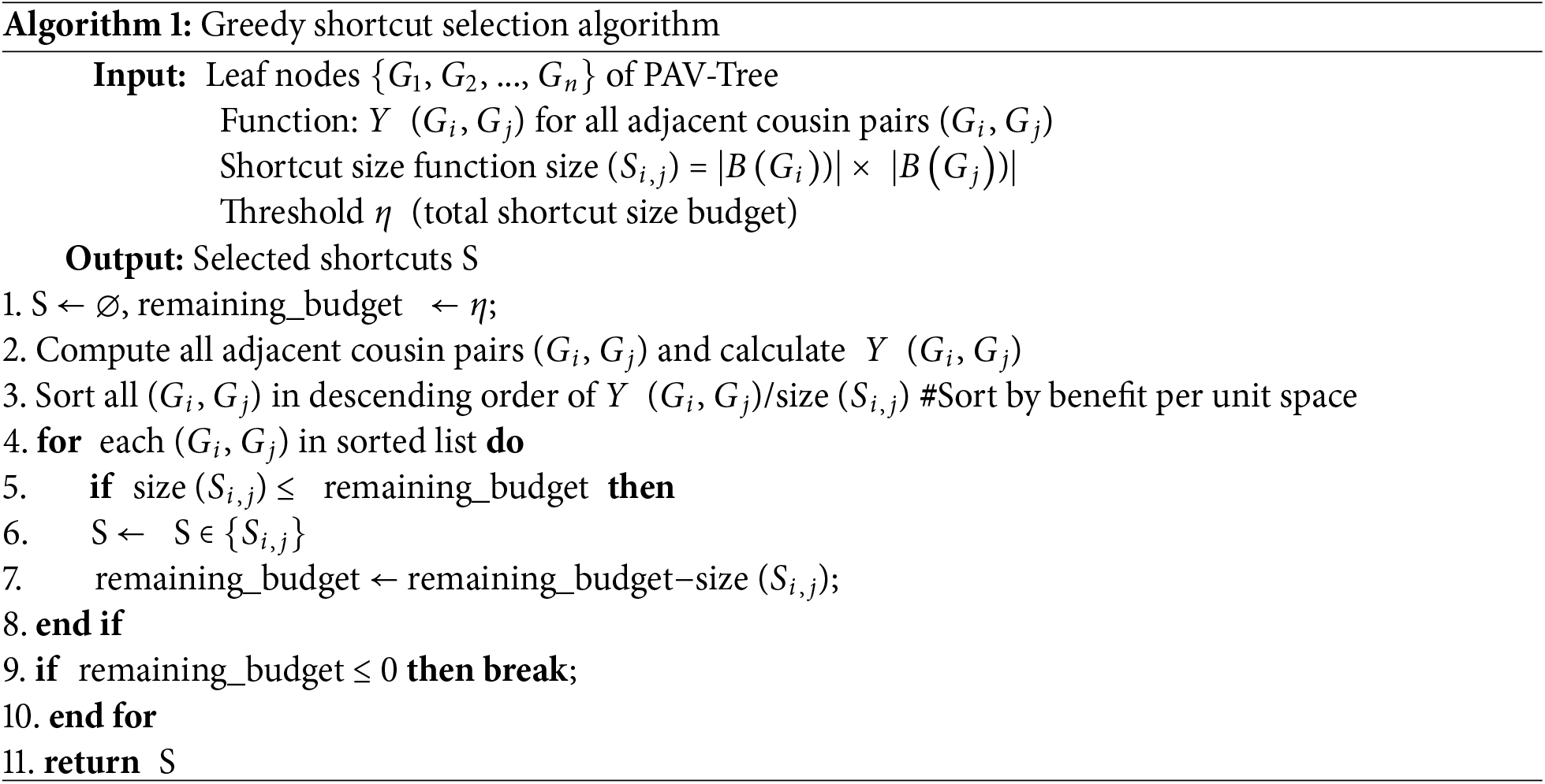
Based on Definition 4, the shortcut selection problem is equivalent to the 0–1 knapsack problem, which is known to be NP-hard. Thus, this paper employs a greedy algorithm to approximate the solution to the shortcut selection problem. The pseudocode for shortcut selection is presented in Algorithm 1.

Example 2 (Building shortcuts for leaf nodes). As an example of the shortcut construction process for the PAV-Tree in Fig. 2b, and based on Definition 1, there are: C∼F, D∼F, and D∼E. Next, we provide a specific example for Y (C, F) using leaf nodes C and F. Note that the SCAP (C, F) is {C,A,B,F}. Thus, the value of the function Y (C, F) is calculated as follows:

Y(C,F)=|B(GC)|+|B(GF)|+|B(GC)|⋅|B(GA)|+|B(GA)|⋅|B(GB)|+|B(GB)|⋅|B(GF)|

=2+1+2×3+3×2+2×1=17.

Similarly, Y (D, F) = 21 and Y (D,E) = 21. Then, based on Definition 4, the shortcut selection problem is formulated as follows:

[Y(C,F),Y(D,F),Y(D,E)]⋅X(4)

[|B(GC)|⋅|B(GF)|,|B(GD)|⋅|B(GF)|,|B(GD)|⋅|B(GE)|]⋅X≤η(5)

Maximize Eq. (4) subject to Eq. (5), where the operator [] denotes the combination of values into a row vector, and X is a column vector that can only take values of 0 or 1. Moreover, in this example, η is set to 5. According to line 3 of Algorithm 1, applying the algorithm yields the sorted list: ((8.5, (GC, GF)), (7, (GD, GE)), (7, (GD, GF))). Finally, substituting the specific values into the above problem yields X = [1,0,1]T. Therefore, this example chooses to create a shortcut between the leaf node pairs <C, F> and <D, E>.

4.4 Comparative Analysis of Index Structures

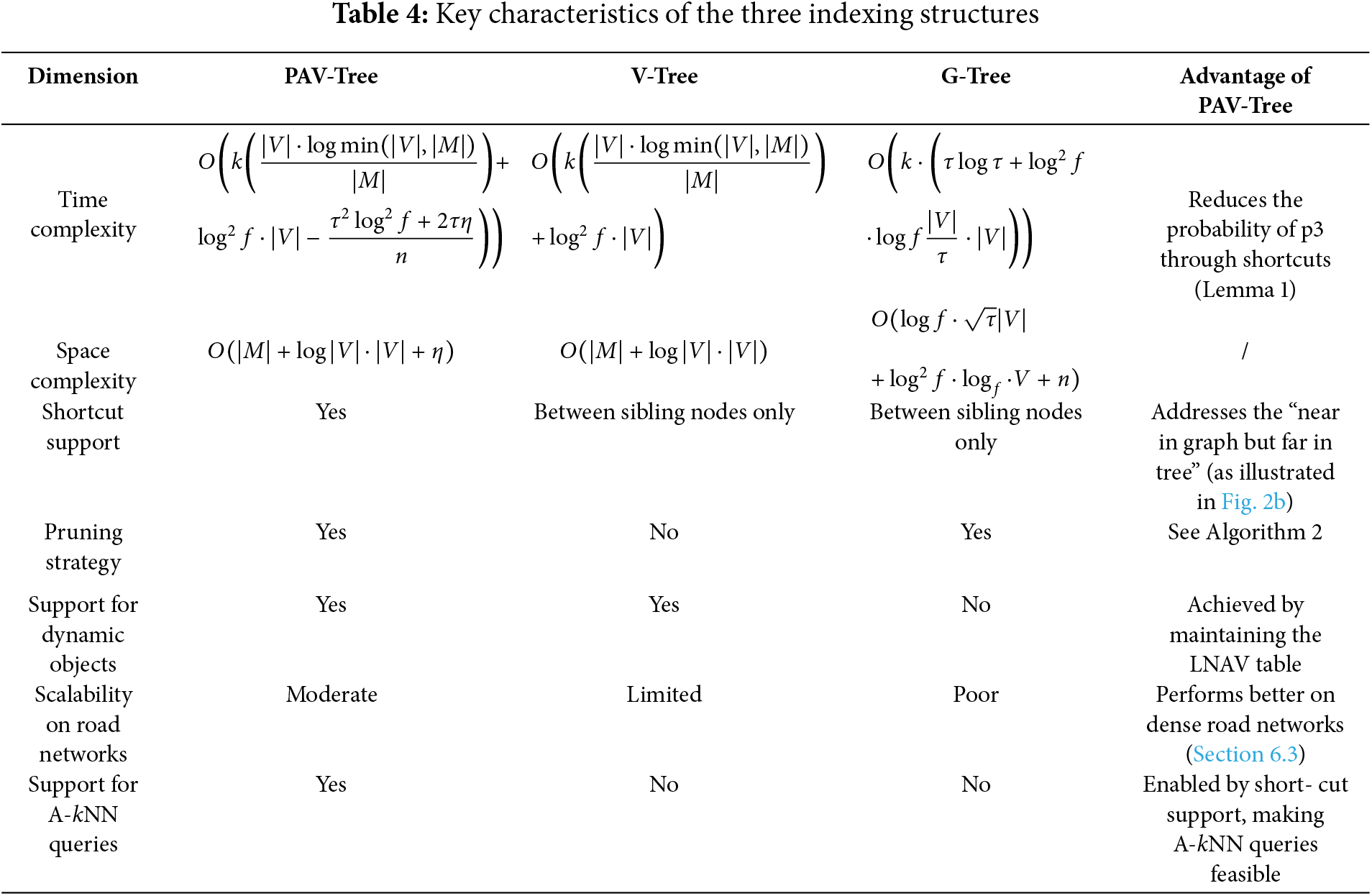
To highlight the structural and functional distinctions among the three major indexing methods—PAV-Tree, V-Tree, and G-Tree—we summarize their key characteristics in Table 4. This comparison not only demonstrates the design improvements introduced by PAV-Tree, such as shortcut support and destination awareness, but also clearly shows its advantages in supporting A-kNN queries and dynamic moving objects.

5  PAV-A-kNN Query Algorithm

5.1 Single-Pair Shortest Path Query

Given a query q = (u,v), the single-pair shortest path query returns SPDist (u,v). As previously noted, existing V-Tree-based methods suffer from redundant computations when calculating the distance between two vertices that are far apart in the V-Tree. In order to resolve this issue, this paper introduces a more efficient approach by utilizing shortcuts in the PAV-Tree, as shown in Algorithm 2. When no shortcut exists between two nodes, the shortest distance is computed using dynamic programming, with the core strategy focused on expanding along the SCAP of the two vertices. During the computation, the algorithm prioritizes visiting boundary vertices and maintains a priority queue to store candidate vertices along the current path, along with their corresponding shortest distances. If a candidate’s distance exceeds the known shortest distance, the algorithm terminates early to avoid redundant calculations.

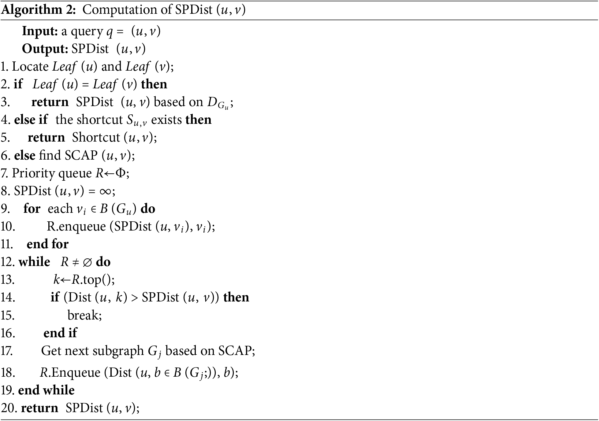
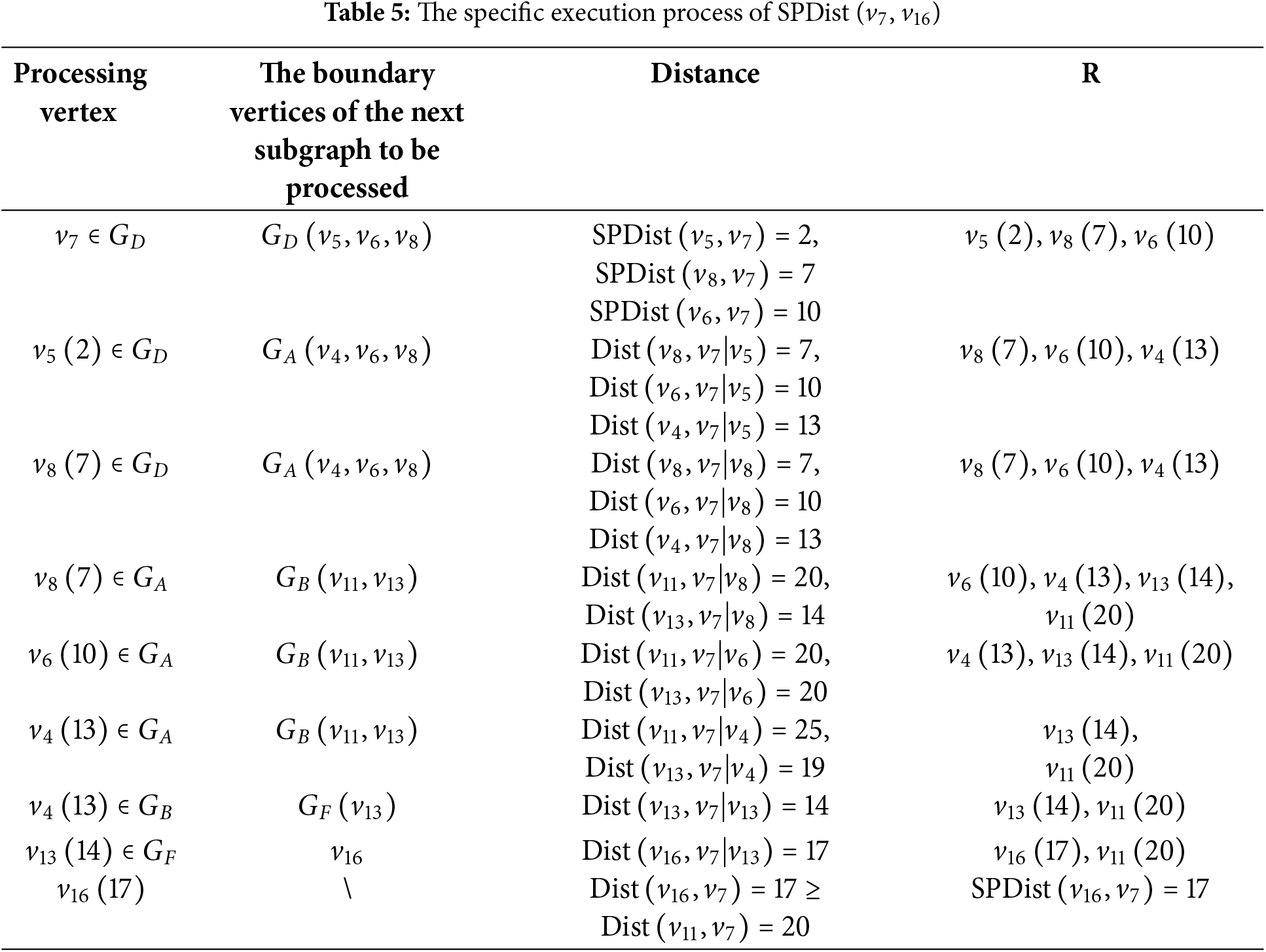
The computation of Algorithm 2 when there is no shortcut between two nodes is given in Fig. 4. It is worth noting that the two red curved lines in Fig. 4 do not need to be computed because at this point, the first element of the queue Dist (v7, v11) = 20 ≥ SPDist (v7, v16) = 17, and the algorithm ends with the return of SPDist (v7, v16) = 17. To provide a clearer explanation, Table 5 presents the detailed procedure for computing SPDist (v7, v16). The notation Dist (u,v|β) refers to the distance from vertex u to vertex v, conditioned on passing through boundary vertex β, as explained in the context of the subgraph structure.

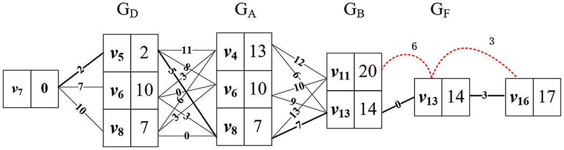
Figure 4: The dynamic programming for computing SPDist (v7, v16)

Lemma 1: The time complexity of Algorithm 2 is:

O(k⋅(τ2V2+τ(1−f)log2⁡f−2τηV+Vlog2⁡f−τ2log2⁡fV))(6)

where V is the number of vertices in the graph, and f, τ and η are the fanout, maximum leaf size and shortcut threshold of the PAV-Tree, respectively.

Proof of Lemma 1. Algorithm 2 is divided into three cases.

1.    Case 1: u and v are in the same subgraph: SPDist (u, v) is directly gotten from leaf distance DGu. The time complexity of this case is O (1).

2.    Case 2: A shortcut exists between leaf (Gu) and leaf (Gv): The time complexity is O (b2), where b denotes the average number of boundary vertices in a leaf node. It has been formally proven in [11] that b = O (τ⋅log⁡f). Thus, in this case, the time complexity is O (τlog2⁡f).

3.    Case 3: No shortcut exists between leaf (Gv) and leaf (Gu): The time complexity is O (nlog2⁡f) [11], so the overall time complexity of Algorithm 2 is:

p1⋅O(1)+p2⋅O(τlog2⁡f)+O(nlog2⁡f)(7)

1.    When two randomly chosen vertices are located within the same subgraph, the probability is given by p1 = τ2n2.

2.    When there is a shortcut between the subgraphs in which the two vertices are located: firstly, the average number of boundaries in each leaf node is τ⋅log⁡f, and each shortcut consumes on average O (τlog2⁡f) space, and each pair of sibling nodes has an implicit shortcut. Therefore, the number of shortcuts is: shortcuts ≈ ητlog2⁡f+f2⋅nτf, where nτf represents the number of parents of all leaf nodes. Secondly, the total number of leaf node pairs is Node Pairs = (n/τ2). Thus, we obtain the probability p2 = shortcutsNodePairs=τ2log2⁡f(f−1)n+2τ2ητlog2⁡f⋅n(n−τ).

3.    It is clear that p3 = (1 − p1 − p2).

Lemma 1 is proved by bringing p1, p2, and p3 into Eq. (7), respectively.

5.2 GNAV Calculation Process

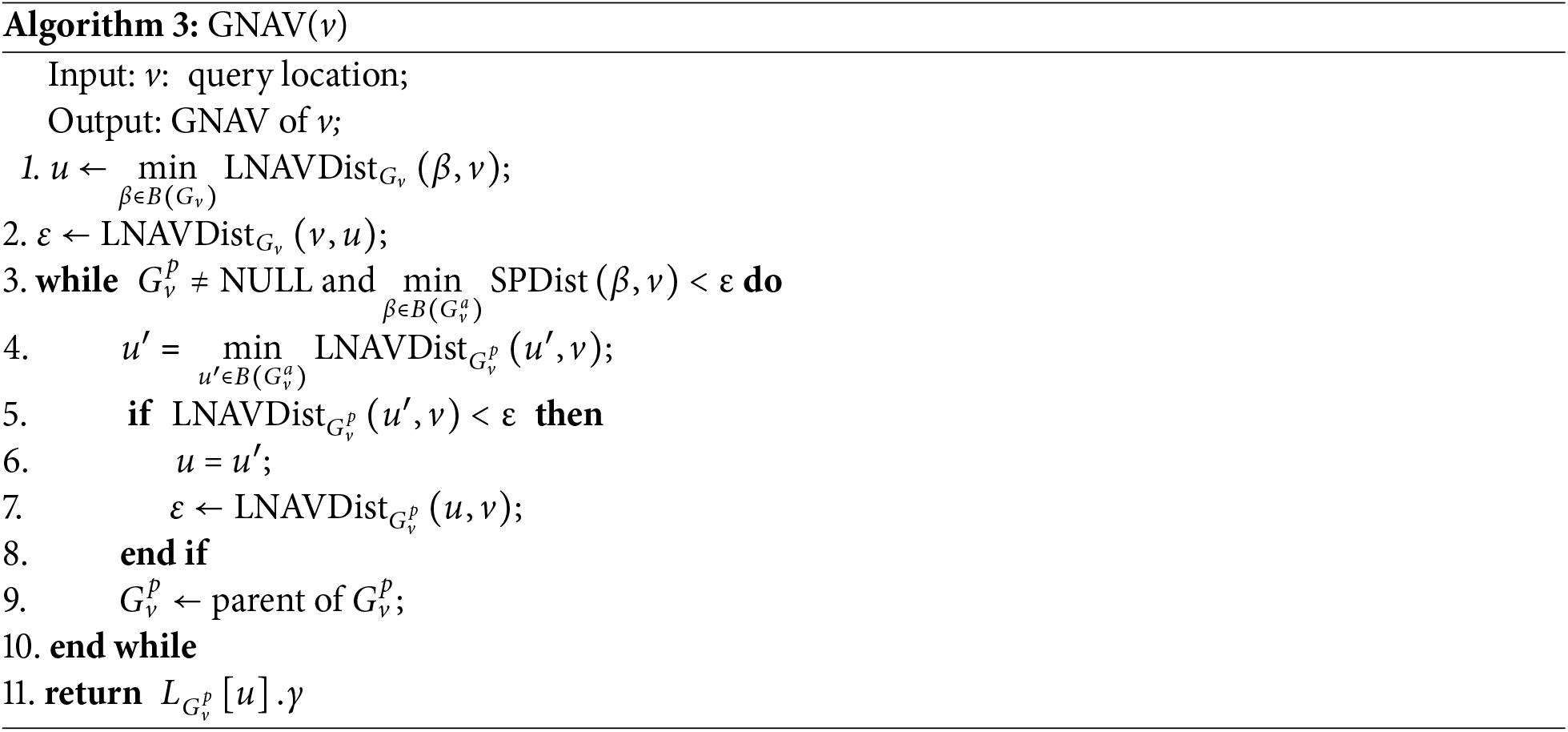
Finding GNAV. This paper employs a bottom-up approach to identify the GNAV, as described in Algorithm 3. The process consists of two main steps:

1.    Exploring the vertices in the leaf graph Gv: Using the LNAV Table LGv of the leaf node Gv, the algorithm identifies the LNAV u of vertex v (line 1 in Algorithm 3) and gets the SPDist(u,v) (line 2).

2.    Exploring boundary vertices of the ancestors of Gv: Let Gvp denote the parent graph of Gv. The variable ε is used to store the minimum distance found so far, and it initialized as LNAVDistGv(u,v). If minβ∈B(Gva)SPDist(β,v)≥ε, the algorithm terminates, as further search would yield active vertices with greater distances. Otherwise, if SPDist (Gvp, v) < ε, the GNAV is identified within Gvp. The algorithm computes smaller active vertex in Gvp (lines 4–7).

Example 3 (Finding the GNAV). Consider finding the GNAV of v6 as an example. First, locate the leaf subgraph GD containing v6. Using the LNAV Table LD of GD, the algorithm determines ε = 8. Next, it searches the locally active vertices in GA. After calculations, the distance from v6 to the active vertex in GA is found to be 3, leading to an update ε = 3. The algorithm then continues to the parent node of GA, which is GR. In GR, it evaluates minβ∈B(GR)SPDist(β,v)=ε = 10. Since this value does not satisfy the loop condition (≥ε), the algorithm terminates. The function returns v3 as the GNAV of v6.

Finding the Next GNAV (NGNAV). To maintain the LNAV table L, the NGNAV(v, u) function is used to identify the next GNAV after the first GNAV has been determined. The main steps are summarized as follows:

Step 1: Deactivation: Mark the current GNAV u as inactive in the PAV-Tree to prevent it from being selected again. Algorithm 3 is then invoked again to continue the identification of subsequent GNAVs.

Step 2: Local Buffer Access: Due to concurrency control, the global LNAV table L cannot be updated during query processing. A local buffer is maintained for each query to store modified entries of L. If the buffer contains valid entries, they are prioritized during retrieval; otherwise, the algorithm falls back to the global L on the PAV-Tree.

Step 3: Query Execution on Modified Graph: The NGNAV computation runs on a slightly modified graph G′, which may cause repeated exploration of unchanged subgraphs. To avoid this, a priority queue (PQ) is used to record boundary vertices along with their LNAVDist values, as detailed in Algorithm 3.

Step 4: Subgraph Reuse Optimization: The algorithm tracks the subgraph GL where the previous GNAV or NGNAV computation terminated. This allows the subsequent NGNAV process to resume traversal from that point, improving efficiency.

Step 5: Early Termination: If the shortest path distance from the query point q to the next candidate u exceeds the threshold ε, the algorithm terminates early to reduce unnecessary computation.

5.3 PAV-A-kNN Algorithm

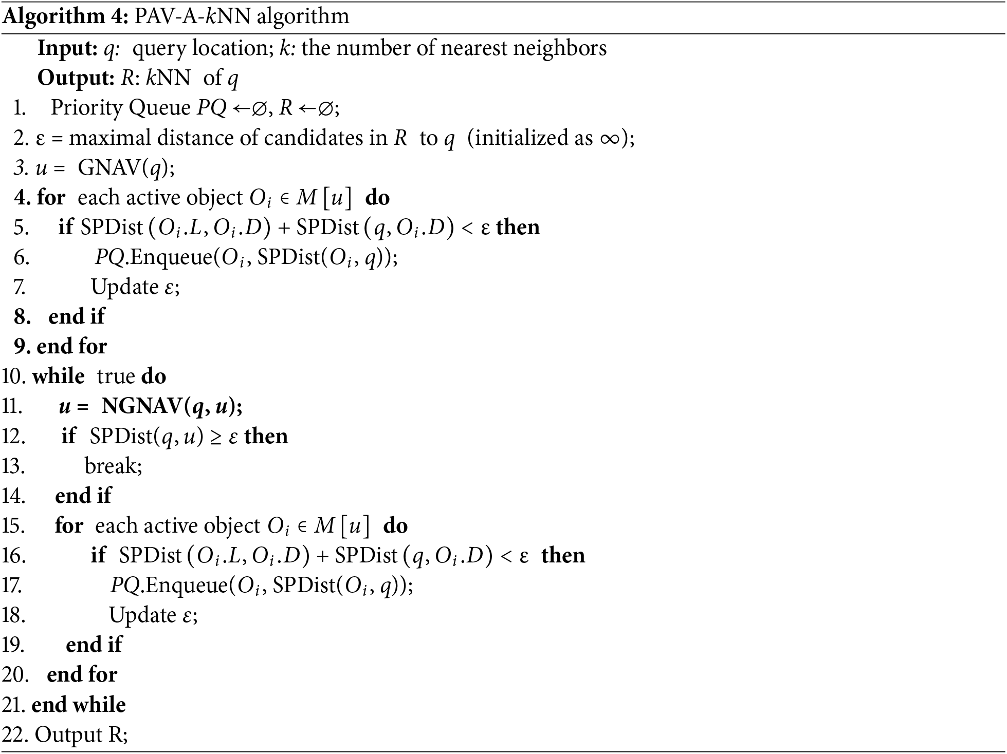
This section introduces the PAV-A-kNN algorithm based on the PAV-Tree. When the destination of a moving object and the query point belong to subgraphs that are far apart, the V-Tree algorithm requires traversing numerous unrelated subgraphs, resulting in inefficient querying of moving objects. To address this, we propose a more efficient algorithm, PAV-A-kNN, as shown in Algorithm 4. The PAV-A-kNN algorithm processes A-kNN queries in three main steps:

1.    Maintaining a priority queue PQ: PQ stores the distances of k candidate objects from the query point q. Initially, ε, which represents the maximum distance of the candidates in PQ to q, is set to ∞ (lines 1–2 in Algorithm 4).

2.    Identifying the First GNAV: By invoking the GNAV(v), the GNAV vertex u for v and SPDist (u,v) are obtained. The Active objects associated with u are added to PQ based on the A-kNN query method, and ε is updated accordingly (lines 3–7).

3.    Locating Subsequent GNAV: Vertex u is marked as inactive, and the NGNAV (v,u) function is called to find the next GNAV. The shortest path distance d = SPDist (u,v) is computed. If d > ε, this indicates that the active objects associated with u cannot be among the kNN results for q, and the algorithm terminates (lines 12–13). Otherwise, the active objects of u are added to PQ (lines 14–18). The process iterates until the top k nearest results are found.

Example 4 (PAV-A-kNN Query): Using PAV-A-kNN (v8, 2) as an example, Fig. 5 illustrates the specific processing steps:

Step 1: The priority queue PQ is initialized as empty (PQ=∅), ε is set to ∞, The function GNAV (v8) is called, returning v5 as the GNAV of v8. The object O2, associated with v5, is added to candidate set R = {(O2, 20)}, ε = 20.

Step 2: The function NGNAV (v8, v5) is called, returning v4. The object O7, associated with v4, is added to R. R = {(O7, 8), (O2, 20)}, ε = 20.

Step 3: The function NGNAV (v8, v4) is called, returning v1. The object O6, associated with v1, is added to R, and ε is updated. R = {(O7, 8), (O6, 11)}, ε = 11.

Step 4: The function NGNAV (v8, v1) is called, returning v2 Since SPDist (v8, v2) = 11 ≥ ε, the algorithm terminates. The final result is R = {(O7, 8), (O6, 11)}.

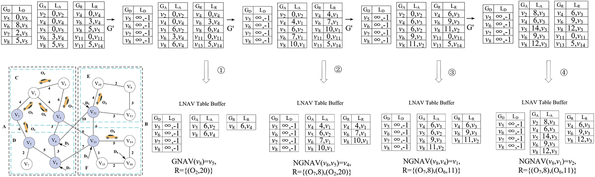
Figure 5: PAV-A-kNN query processing steps for (v8, 2)

5.4 Time Complexity of the PAV-A-kNN Algorithm

Given a graph G and PAV-Tree with V vertices and M moving objects, with the assumption that the moving objects are uniformly distributed across the road network, the average time complexity of A-kNN search is:

O(k⋅(Vlog2⁡f+Vlog⁡min(V,M)M))(8)

6  Experiment

Datasets: We evaluated the proposed algorithm using eight different datasets, including both synthetic and real-world datasets, as shown in Table 6.

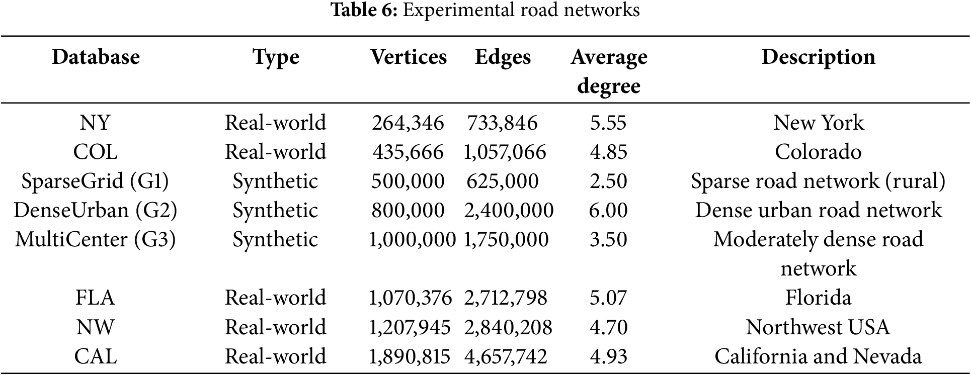
Environment. All experiments were carried out on a computer running Windows 11, with an Intel i5-9300H CPU (2.40 GHz), 8 GB RAM, and a 512 GB SSD. The experiments were carried out within a virtual machine configured with 4 GB of memory and two processors, each with two cores (a total of four cores). All algorithms were implemented in C++, without utilizing any parallelization techniques; all programs were executed serially on a single core. Graph partitioning was performed using the METIS library. The indexing structures were implemented based on adjacency lists, and all methods were evaluated under identical experimental conditions.

Baseline: We compared PAV-Tree, with the methods of V-Tree [5] and G-Tree [11], and the three index structures were set with fanout f = 4 and τ = 32, which are the same as the V-Tree proposed parameters. Additionally, the shortcut threshold η for the PAV-Tree was set as follows: 1 million for NY, COL, G1, and G2; 1.5 million for G3, FLA, NW; and 3.5 million for CAL. These values were chosen to ensure that the size of the shortcuts does not exceed approximately 15% of the total size of the PAV-Tree.

Moving Objects: The density of moving objects was uniformly set to θ − TotalnumberofmovingobjectsTotalnumberofvertices = 0.01. Additionally, 90% of the moving objects were configured to be in an occupied state. For unoccupied objects, their destinations were set to ∅. The positions of moving objects were randomly generated.

6.1 Evaluation on Index Construction

This section evaluates the index construction cost and index size of PAV-Tree, V-Tree, and G-Tree across the eight datasets.

Fig. 6 presents a comparison of the construction time and space consumption for the three index structures. The results show that both construction time and index size increase with the scale of the dataset. In terms of construction time, PAV-Tree falls between V-Tree and G-Tree. Although PAV-Tree incurs slightly higher overhead than V-Tree due to the additional cost of building shortcuts between leaf nodes, its bottom-up construction strategy effectively avoids redundant computations, resulting in better construction efficiency than G-Tree. Regarding index size, the differences among the three methods are relatively small. PAV-Tree’s index is marginally larger, as it stores additional information, such as moving objects and inter-leaf shortcuts.

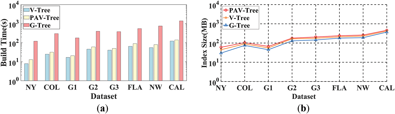
Figure 6: Index comparison. (a) Construction time. (b) Index size

It is worth noting that on dense graphs (e.g., G2, FLA, and CAL), both index construction time and space usage grow more significantly. This is mainly due to higher vertex connectivity, which increases the number of border vertices and the complexity of shortcut construction. In contrast, for sparse graphs (e.g., G1), where the network structure is simpler, the differences in index construction time and space consumption among the three methods are less pronounced. Overall, PAV-Tree demonstrates a good balance between efficiency and scalability across both sparse and dense road networks.

6.2 Evaluation of A-kNN Query Performance

This section evaluates the A-kNN query performance of the PAV-Tree, V-Tree, and G-Tree on the NW dataset. The experiments were conducted by varying parameters such as the values of k, query distances, update intervals, and the densities of moving objects. Let there be n queries, q1, …, qn, within a specified time period, and assume that objects are updated before executing each qi. The average total query time is calculated as follows: Average Total Query Time = Tu+∑i=1nTqin, where Tu represents the update time and Tq denotes the query time for each query Ti. In the bar charts, the entire bar represents the total query time, with the top part showing the average update time and the bottom part showing the average query time.

Varying K: As shown in Fig. 7a, we conducted experiments with varying k values, ranging from 10 to 50 in increments of 10. The results clearly demonstrate that the PAV-Tree consistently achieves the fastest query times. This is because PAV-Tree can efficiently utilize the LNAV Table L to quickly locate moving objects. Additionally, when a moving object is already occupied, PAV-Tree utilizes shortcuts to rapidly compute the actual distance between the query point and the moving object. In contrast, the V-Tree approach may unnecessarily traverse multiple leaf nodes when calculating the actual distance, which significantly impacts its efficiency. Among the three algorithms, G-Tree is the slowest, as it traverses the tree structure in a top-down manner, requiring substantial computation and incurring high cost to explore its subtrees.

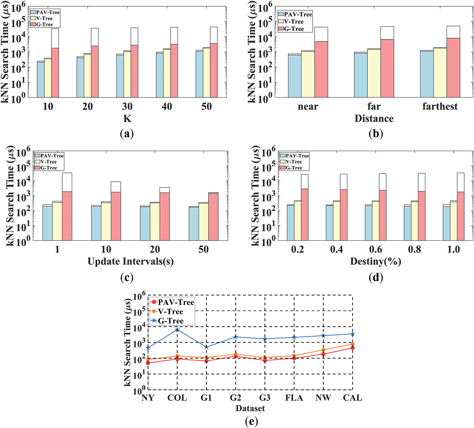
Figure 7: Performance comparison of A-kNN queries (NW Dataset(a-e)). (a) Varying K, (b) Varying distance, (c) Varying updating interval, (d) Varying density, (e) Performance comparison of A-kNN on different datasets.

Varying Distance: For different query distances, we first extract the query location from the actual query, and then sort the objects according to their distance from the query location. The moving objects are categorized into three groups of equal size: near, far, and farthest, with k set to 10. The experimental results, as shown in Fig. 7b, indicate that the average total search time of all three algorithms tends to increase as the query distance increases. However, PAV-Tree always maintains the best performance. Specifically, for long-distance queries, the PAV-Tree algorithm performs better by accessing fewer tree nodes and utilize shortcuts to efficiently calculate the distance between the query point and the moving object.

Varying Update Interval: For update intervals, we set the values to 1, 10, 20, and 50 s, with k set to 10. We evaluated the update cost using the positions of moving objects and queries during this period. The results presented in Fig. 7c indicate that as the update frequency decreases, the average update time for all three algorithms decreasing accordingly. This is because the cost of updates decreases with longer update intervals.

Varying Density: For the density of moving objects, we tested values of 0.2%, 0.4%, 0.6%, 0.8%, and 1.0%, with k set to 10. The results are shown in Fig. 7d. First, in terms of search time, the performance of PAV-Tree is always optimal. Second, with the increase in the number of search objects, the average total query time for all three algorithms also grows. This is attributed to the increased update overhead caused by the growing number of moving objects. Additionally, all three algorithms achieve faster average query speeds while increasing object density, as higher density reduces search space.

Various Datasets: To assess the query efficiency of the three algorithms, we measured the average response time for single queries across eight distinct datasets, with the parameter k fixed at 10. As illustrated in Fig. 7e, the PAV-Tree consistently achieves superior performance, exhibiting nearly a 50% reduction in query time compared to the V-Tree, and outperforming the G-Tree by one to two orders of magnitude. This notable improvement stems from the shortcut connections established between leaf nodes during the PAV-Tree’s index construction phase, which improves the efficiency of computing the actual distance between the query point and moving objects.

6.3 Scalability Evaluation under Varying Workloads

To comprehensively assess the performance and scalability of the three query methods, we conducted experiments under both normal and extreme conditions. These tests evaluate the method’s adaptability to diverse road network structures and its efficiency in handling high-density moving objects with frequent updates.

6.3.1 Normal Workload Scenario

We conducted a comparative evaluation of PAV-A-kNN against two baseline methods under standardized testing conditions, with fixed parameters (k = 10, vehicle density = 1%, update interval = 1 s) as shown in Fig. 8a.

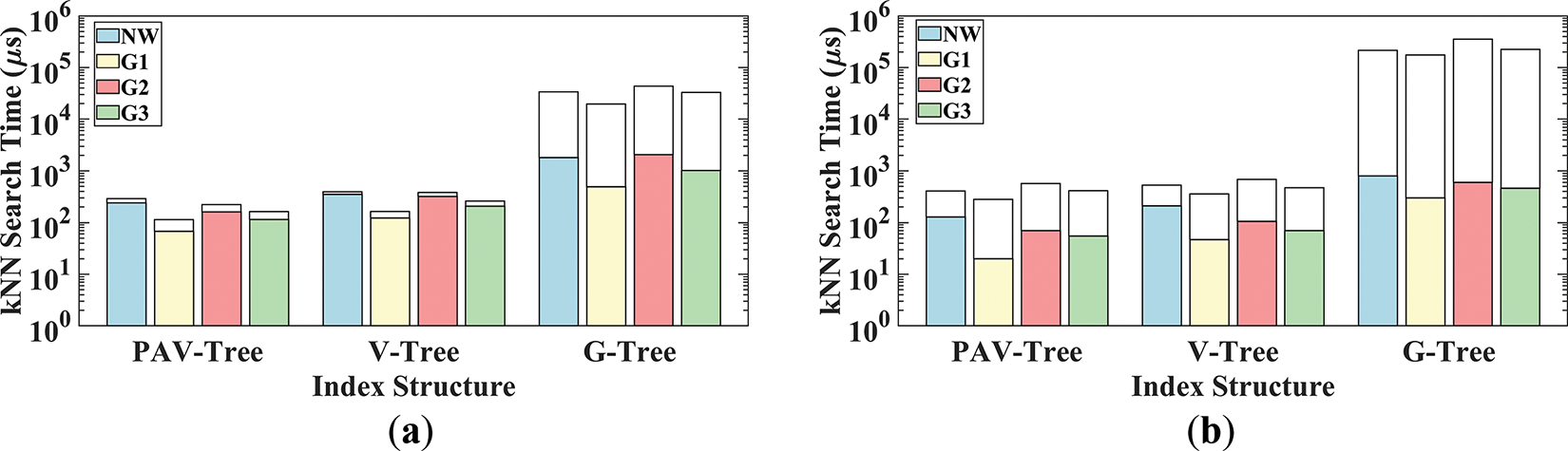
Figure 8: Performance evaluation under varying workload conditions. (a) Standard workload; (b) Stress workload

Query Efficiency: PAV-Tree achieves query times of 58–210 μs, which is 35%–60% faster than V-Tree and 3%–12% of G-Tree’s query time. In Sparse graph (G1), PAV-Tree has a high shortcut coverage, thus achieving the lowest query latency (58 μs). In the dense graph (G2), although the number of boundary vertices increases, causing queries to traverse more vertices, the PAV-Tree maintains efficient querying (141 μs). In contrast, the absence of dynamic pruning mechanisms in V-Tree results in significant performance degradation (320 μs), while G-Tree suffers from severe computational overhead (1560 μs) due to its exhaustive subgraph exploration pattern.

Update Efficiency: PAV-Tree’s update times (46–72 μs) are comparable to V-Tree, while G-Tree’s global index reconstruction leads to 2 orders of magnitude higher overhead (19.2–41.6 ms). The slightly higher update time for G2 (62 μs vs. 46 μs for G1) is due to prolonged LNAV table updates in dense networks.

6.3.2 Extreme Workload Scenario

To evaluate robustness, we tested the algorithm under high-density moving objects and frequent updates: uniformly set parameters: k = 10, the density of moving objects is 10%, and the update interval is 0.2 s. The result is shown in Fig. 8b. As moving object density and update frequency increase, all methods exhibit reduced query times but significantly higher update overhead (see Section 6.2), but still within the range of real-time operation.

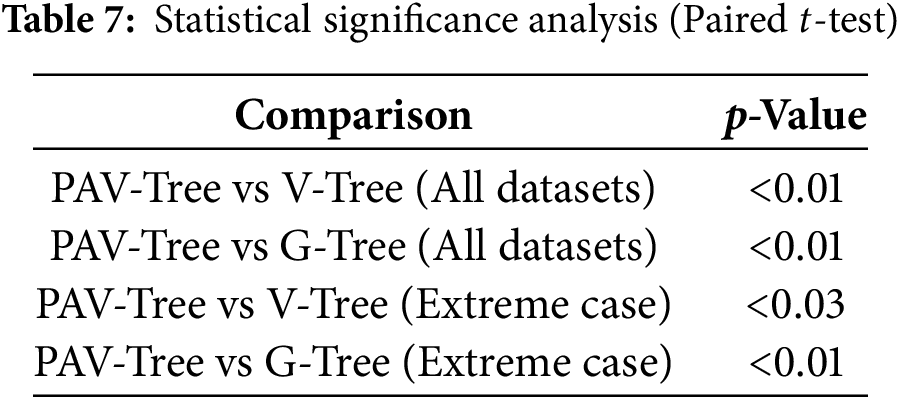
To confirm the statistical significance of these improvements, we repeated the experiments in Figs. 7e and 8b five times and conducted paired t-tests. As shown in Table 7, even in the most extreme cases, all observed improvements were statistically significant (p < 0.05).

6.4 Evaluation of Shortcut Parameter η

In this section, we evaluate the impact of shortcut selection parameters on the query efficiency of the PAV-Tree. Specifically, we design two sets of experiments to investigate: (1) the effect of different shortcut threshold configurations, and (2) the influence of shortcut usage on algorithm execution time.

6.4.1 Performance Evaluation of Shortcut

In the first set of experiments, we compared the execution time of PAV-Tree with and without the shortcut mechanism on four road network datasets (NW, G1, G2, and G3), which exhibit diverse topological structures and density characteristics. The results, shown in Fig. 9a, indicate that enabling the shortcut mechanism significantly reduces query time across all datasets, achieving an average speedup of approximately 2.2×. The G1 dataset achieves the highest improvement, with query time reduced from 150 to 68 μs. This is primarily due to the sparsity of the graph, where fewer direct connections between vertices result in longer path dependencies; thus, shortcuts can bypass redundant computations more effectively. In contrast, the performance gain on dense graphs (e.g., G2) is relatively limited. In such networks, the abundance of direct edges between vertices reduces the marginal utility of additional shortcuts. These findings further validate the critical role of shortcuts in accelerating the query process, particularly in medium- to large-scale graphs. Furthermore, the varying levels of improvement across datasets suggest that the effectiveness of shortcut-based optimization is more pronounced in sparse graphs and networks with high path selection complexity.

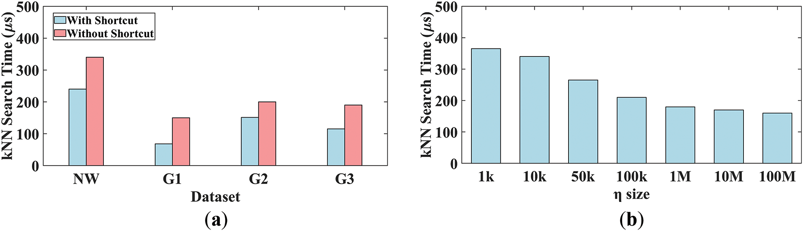
Figure 9: Performance evaluation of shortcut. (a) With/without shortcut. (b) Varying shortcut thresholds η

6.4.2 Query Performance under Varying Shortcut Thresholds

We evaluated the query performance of PAV-Tree on NW dataset under different shortcut thresholds, with the threshold values ranging from 1 k to 100 M. As shown in Fig. 9b, the execution time decreases significantly with the increase of the shortcut threshold, dropping from 340 to 160 μs. The most notable performance improvement is observed when the threshold increases from 10 to 10 and 100 k. This indicates that increasing the threshold will skip the calculation of actual path extension and shortest path during query processing, thereby improving query efficiency. However, when the number of shortcuts reaches a certain scale (such as 10 to 100 M), the improvement in query performance begins to reach saturation. This is because as shortcuts become increasingly dense, the types and distribution of covered paths are already sufficient, and the original paths are close to optimal in space, making it difficult to further significantly optimize query performance.

6.5 Real-Time Feasibility Analysis

In ride-hailing systems, real-time responsiveness is critical, with typical requirements demanding sub-second latency. As shown in Fig. 7e, the proposed PAV-A-kNN algorithm achieves average query times at the microsecond (μs) level, even on large-scale datasets such as CAL and NW. For instance, the average response time on the CAL dataset is approximately 553 μs. This ultra-low latency indicates that our method not only meets the sub-second responsiveness requirement but also leaves sufficient headroom for additional computation or integration overhead. Therefore, it is highly suitable for practical deployment in high-demand environments, such as online ride-hailing platforms.

6.6 Runtime Breakdown Analysis of the PAV-A-kNN Algorithm

To validate the efficiency of each component in PAV-A-kNN, we analyze the runtime distribution across datasets with varying road network densities (with the same query conditions as Section 6.3.1). Table 8 presents the detailed breakdown of query time for GNAV computation, shortcut processing, and other operations (e.g., priority queue updates and shortest path calculations).

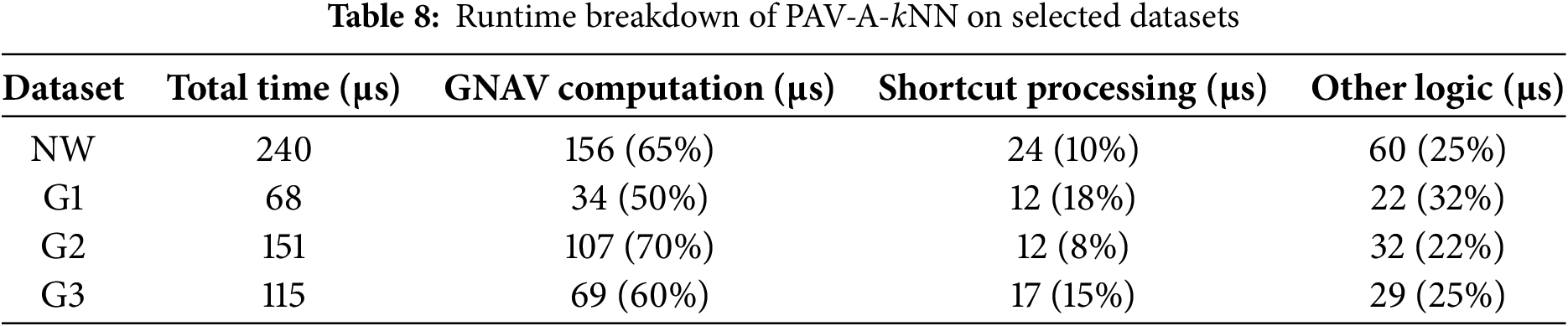
Across four representative datasets, GNAV computation consistently constitutes the primary source of runtime overhead. In particular, it accounts for 70% on the dense graph G2 and 65% on the real-world road network NW, indicating the high cost of locating the nearest active object in complex graph structures. On the sparse graph G1, the GNAV share drops to 50%, while shortcut processing increases to 18%, suggesting that shortcuts are more effective in accelerating queries when the path selection space is limited. The overhead of control logic—including priority queue maintenance and LNAV buffer updates—remains stable across datasets, ranging from 22% to 32%.

Overall, PAV-A-kNN spends the majority of its runtime on GNAV-related search, while shortcut processing incurs minimal overhead but shows notable effectiveness in sparse networks. Control logic remains a consistent cost component. These findings confirm the efficiency and adaptability of the algorithm across different graph structures.

7  Conclusions

In this paper, we investigate a novel type of kNN query method, known as Approachable kNN (A-kNN) query which differs from traditional kNN methods in the measurement between the query points and the moving objects. Although V-Tree is widely recognized as an efficient kNN method, its limitations in computing the shortest distance between arbitrary vertices make it less efficient in handling A-kNN queries. To address the efficiency limitations of existing methods, a novel indexing structure, PAV-Tree, is proposed. It extends the V-Tree by establishing shortcuts between leaf nodes thereby accelerating the shortest distance queries between vertices. In addition, an efficient PAV-A-kNN algorithm is developed to solve the A-kNN query problem. Finally, we conduct extensive experiments on both real-world and synthetic datasets, with empirical results demonstrating that our proposed method achieves significant advantages over baseline approaches. Despite its promising performance, the proposed method still presents several challenges. First, space overhead may become a bottleneck in large-scale networks, as the storage of numerous shortcuts can be prohibitive. This limitation highlights the need for more efficient shortcut selection or compression strategies. Second, the index’s robustness under noisy data—such as imprecise vertex coordinates or corrupted edge weights—has not been thoroughly examined. Addressing this issue could further improve the reliability of A-kNN queries in real-world settings. While these issues merit attention, our immediate future work will focus on two key directions: (1) extending the approach to dynamic road networks, where edge weights vary over time; and (2) exploring learning-based methods for shortest path estimation, such as leveraging graph neural networks (GNNs) or reinforcement learning (RL), to enhance query efficiency and reduce redundant path traversal.

Acknowledgement: The authors gratefully acknowledge all those who contributed to the research and preparation of this article.

Funding Statement: This work was supported by the Special Project of Henan Provincial Key Research, Development and Promotion (Key Science and Technology Program) under Grant 252102210154, in part by the National Natural Science Foundation of China under Grant 62403437.

Author Contributions: Conceptualization, Kailai Zhou and Weikang Xia; Methodology, Weikang Xia; Software, Weikang Xia; Validation, Kailai Zhou; Formal analysis, Jiatai Wang; Data Curation, Kailai Zhou; Writing—original draft preparation, Weikang Xia; Writing—review & editing, Weikang Xia; Supervision, Jiatai Wang. All authors reviewed the results and approved the final version of the manuscript.

Availability of Data and Materials: The data that support the findings of this study are available from the corresponding author, K.Z., upon reasonable request.

Ethics Approval: Not applicable.

Conflicts of Interest: The authors declare no conflicts of interest to report regarding the present study.

References

1. Sarana N, Rui Z, Egemen T, Lars K. The V*-Diagram: a query-dependent approach to moving KNN queries. Proc VLDB Endow. 2008;1(1):1095–106. doi:10.14778/1453856.1453973. [Google Scholar] [CrossRef]

2. He D, Wang S, Zhou X, Cheng R. An efficient framework for correctness-aware kNN queries on road networks. In: 2019 IEEE 35th International Conference on Data Engineering (ICDE); 2019 Apr 8–11; Macao, China . p. 1298–309. doi:10.1109/icde.2019.00118. [Google Scholar] [CrossRef]

3. Cho HJ. The efficient processing of moving k-farthest neighbor queries in road networks. Algorithms. 2022;15(7):223. doi:10.3390/a15070223. [Google Scholar] [CrossRef]

4. Li M, He D, Zhou X. Efficient kNN search with occupation in large-scale on-demand ride-hailing. In: Databases theory and applications. Cham, Switzerland: Springer International Publishing; 2020. p. 29–41. doi:10.1007/978-3-030-39469-1_3. [Google Scholar] [CrossRef]

5. Shen B, Zhao Y, Li G, Zheng W, Qin Y, Yuan B, et al. V-tree: efficient kNN search on moving objects with road-network constraints. In: 2017 IEEE 33rd International Conference on Data Engineering (ICDE); 2017 Apr 19–22; San Diego, CA, USA. p. 609–20. doi:10.1109/ICDE.2017.115. [Google Scholar] [CrossRef]

6. Feng Q, Zhang J, Zhang W, Qin L, Zhang Y, Lin X. Efficient kNN search in public transportation networks. Proc VLDB Endow. 2024;17(11):3402–14. doi:10.14778/3681954.3682009. [Google Scholar] [CrossRef]

7. Jiang W, Ning B, Li G, Bai M, Jia X, Wei F. Graph-decomposed k-NN searching algorithm on road network. Front Comput Sci. 2024;18(3):183609. doi:10.1007/s11704-023-3626-3. [Google Scholar] [CrossRef]

8. Xu Y, Zhang M, Wu R, Li L, Zhou X. Efficient processing of coverage centrality queries on road networks. World Wide Web. 2024;27(3):25. doi:10.1007/s11280-024-01248-5. [Google Scholar] [CrossRef]

9. Min X, Pfoser D, Züfle A, Sheng Y, Huang Y. The partition bridge (PB) tree: efficient nearest neighbor query processing on road networks. Inf Syst. 2023;118(5):102256. doi:10.1016/j.is.2023.102256. [Google Scholar] [CrossRef]

10. Dijkstra EW. A note on two problems in connexion with graphs. Numer Math. 1959;1(1):269–71. doi:10.1007/BF01386390. [Google Scholar] [CrossRef]

11. Zhong R, Li G, Tan KL, Zhou L, Gong Z. G-tree: an efficient and scalable index for spatial search on road networks. IEEE Trans Knowl Data Eng. 2015;27(8):2175–89. doi:10.1109/TKDE.2015.2399306. [Google Scholar] [CrossRef]

12. Li Z, Chen L, Wang Y. G*-tree: an efficient spatial index on road networks. In: 2019 IEEE 35th International Conference on Data Engineering (ICDE); 2019 Apr 8–11; Macao, China. p. 268–79. doi:10.1109/ICDE.2019.00032. [Google Scholar] [CrossRef]

13. Li L, Cheema MA, Ali ME. Continuously monitoring alternative shortest paths on road networks. In: vLDB endowment. 3rd edition. New York, NY, USA: Association for Computing Machinery; 2020. p. 2243–55. doi:10.14778/3407790.3407822. [Google Scholar] [CrossRef]

14. Abeywickrama T, Cheema MA, Storandt S. Hierarchical graph traversal for aggregate k nearest neighbors search in road networks. In: Proceedings of the International Conference on Automated Planning and Scheduling; 2020 Jun 14–19; Nancy, France. p. 2–10. doi:10.1609/icaps.v30i1.6639. [Google Scholar] [CrossRef]

15. Luo S, Kao B, Li G, Hu J, Cheng R, Zheng Y. Toain: a throughput optimizing adaptive index for answering dynamic knn queries on road networks. Proc VLDB Endow. 2018;11(5):594–606. doi:10.1145/3177732.3177736. [Google Scholar] [CrossRef]

16. He D, Wang S, Zhou X, Cheng R. GLAD: a grid and labeling framework with scheduling for conflict-aware kNN queries. IEEE Trans Knowl Data Eng. 2021;33(4):1554–66. doi:10.1109/TKDE.2019.2942585. [Google Scholar] [CrossRef]

17. Geisberger R, Sanders P, Schultes D, Delling D. Contraction hierarchies: faster and simpler hierarchical routing in road networks. In: Experimental Algorithms. Berlin/Heidelberg, Germany: Springer; 2008. p. 319–33. doi:10.1007/978-3-540-68552-4_24. [Google Scholar] [CrossRef]

18. Ouyang D, Qin L, Chang L, Lin X, Zhang Y, Zhu Q. When hierarchy meets 2-hop-labeling: efficient shortest distance queries on road networks. In: Proceedings of the 2018 International Conference on Management of Data; 2018; Houston, TX, USA. p. 709–24. doi:10.1145/3183713.3196913. [Google Scholar] [CrossRef]

19. Ouyang D, Wen D, Qin L, Chang L, Zhang Y, Lin X. Progressive top-K nearest neighbors search in large road networks. In: Proceedings of the 2020 ACM SIGMOD International Conference on Management of Data; 2020; Portland, OR, USA. p. 1781–95. doi:10.1145/3318464.3389746. [Google Scholar] [CrossRef]

20. Wang Y, Yuan L, Zhang W, Lin X, Chen Z, Liu Q. Simpler is more: efficient top-K nearest neighbors search on large road networks. arXiv:2408.05432, 2024. [Google Scholar]

21. Wang S, Xiao X, Yang Y, Lin W. Effective indexing for approximate constrained shortest path queries on large road networks. Proc VLDB Endow. 2016;10(2):61–72. doi:10.14778/3015274.3015277. [Google Scholar] [CrossRef]

22. Zhu AD, Xiao X, Wang S, Lin W. Efficient single-source shortest path and distance queries on large graphs. In: Proceedings of the 19th ACM SIGKDD International Conference on Knowledge Discovery and Data Mining; 2013; Chicago, IL, USA. p. 998–1006. doi:10.1145/2487575.2487665. [Google Scholar] [CrossRef]

23. Singh A. A novel shortest path problem using dijkstra algorithm in interval-valued neutrosophic environment. In: 2022 International Conference on Smart Generation Computing, Communication and Networking (SMART GENCON); 2022 Dec 23–25; Bangalore, India. p. 1–6. doi:10.1109/SMARTGENCON56628.2022.10083619. [Google Scholar] [CrossRef]

24. Wang L, Wong RC. PCSP: efficiently answering label-constrained shortest path queries in road networks. Proc VLDB Endow. 2024;17(11):3082–94. doi:10.14778/3681954.3681985. [Google Scholar] [CrossRef]

25. Li J, Chen Y, Zhang M, Li L. A CPU-GPU hybrid labelling algorithm for massive shortest distance queries on road networks. Proc VLDB Endow. 2024;18(3):770–83. doi:10.14778/3712221.3712241. [Google Scholar] [CrossRef]

26. Chen Z, Fu AW, Jiang M, Lo E, Zhang P. P2H: efficient distance querying on road networks by projected vertex separators. In: Proceedings of the 2021 International Conference on Management of Data. Virtual Event; 2021; China. p. 313–25. doi:10.1145/3448016.3459245. [Google Scholar] [CrossRef]

27. Anirban S, Wang J, Islam MS. Experimental evaluation of indexing techniques for shortest distance queries on road networks. In: 2023 IEEE 39th International Conference on Data Engineering (ICDE); 2023 Apr 3–7; Anaheim, CA, USA. p. 624–36. doi:10.1109/ICDE55515.2023.00054. [Google Scholar] [CrossRef]

28. Dan T, Luo C, Li Y, Guan Z, Meng X. LG-tree: an efficient labeled index for shortest distance search on massive road networks. IEEE Trans Intell Transp Syst. 2022;23(12):23721–35. doi:10.1109/TITS.2022.3203432. [Google Scholar] [CrossRef]

29. Huang S, Wang Y, Zhao T, Li G. A learning-based method for computing shortest path distances on road networks. In: 2021 IEEE 37th International Conference on Data Engineering (ICDE); 2021 Apr 19–22; Chania, Greece. p. 360–71. doi:10.1109/icde51399.2021.00038. [Google Scholar] [CrossRef]

30. Zheng B, Ma Y, Wan J, Gao Y, Huang K, Zhou X, et al. Reinforcement learning based tree decomposition for distance querying in road networks. In: 2023 IEEE 39th International Conference on Data Engineering (ICDE); 2023 Apr 3–7; Anaheim, CA, USA. p. 1678–90. doi:10.1109/ICDE55515.2023.00132. [Google Scholar] [CrossRef]

31. Drakakis S, Kotropoulos C. Applying the neural bellman-ford model to the single source shortest path problem. In: Proceedings of the 13th International Conference on Pattern Recognition Applications and Methods; 2024 Feb 24–26; Rome, Italy. p. 386–93. doi:10.5220/0012425800003654. [Google Scholar] [CrossRef]