SP-Sketch: Persistent Flow Detection with Sliding Windows on Programmable Switches

1  Introduction

Persistent flow detection is fundamental for uncovering long-term abnormal traffic patterns, including low-rate denial-of-service (LDoS) attacks, network probing, and malicious activities [1–3]. Unlike transient anomalies, persistent flows—defined as those appearing in at least k distinct time intervals (where k is a predefined operational threshold)—manifest recurrent patterns over extended periods, often with negligible traffic intensity. Detecting persistent flows is indispensable for network performance monitoring and security, as they frequently signal underlying issues like misconfigurations or stealthy attacks [4].

However, existing persistent flow detection solutions typically encounter substantial trade-offs between accuracy and memory efficiency, especially in real-time, high-speed network environments. Traditional methods, such as fixed-window sketches [5] and multi-instance tracking, often suffer from prohibitive memory overhead and computational limitations, making them challenging to deploy efficiently in high-throughput networks. This issue is particularly pronounced in programmable switches (e.g., P4 devices), where the strict limitations on memory and computational resources make existing solutions fundamentally incompatible (e.g., Tofino ASIC only has 15 MB SRAM and limited ALUs, and does not support floating-point numbers or division operations) [6].

Specifically, as shown in Fig. 1, conventional sliding window methods typically require multiple sketch instances to represent sub-intervals within a time window, with each instance maintaining independent flow counters. This design not only substantially increases memory consumption but also introduces significant computational overhead, especially in network environments requiring real-time processing. Programmable switches, with their fixed pipeline architecture, are fundamentally constrained in their ability to maintain long-term state or perform complex computations, further exacerbating this challenge [7].

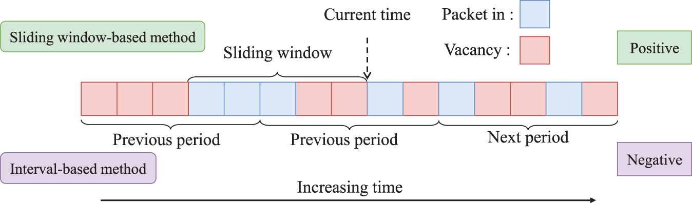
Figure 1: Comparison of sliding window and interval-based window techniques for persistent flow detection

Therefore, a key question arises: Considering the limitations of programmable switches, can we efficiently detect multiple persistent flows, ensuring high accuracy and temporal resolution without requiring excessive memory and computational resources?

To address this fundamental challenge, we propose SP-Sketch, a memory-efficient sketch-based method for real-time persistent flow detection on programmable switches, using an innovative sliding window scheme. SP-Sketch integrates the advantages of sliding window techniques with an innovative probabilistic subtraction mechanism to provide accurate persistent flow estimation without requiring multiple sketch instances or timestamp storage. The core innovation of SP-Sketch lies in its ability to dramatically reduce memory requirements by maintaining a single sketch structure, where counter values are probabilistically incremented or decremented based on flow occurrences, precisely simulating the expiration of historical data without additional memory overhead. This approach enables precise persistent flow detection with minimal memory utilization, making it particularly suitable for deployment in resource-constrained, real-time environments.

The main contributions of this paper are summarized as follows:

•   We propose SP-Sketch, a novel sliding window-based persistent flow measurement solution that simulates slot expiration using a probabilistic subtraction mechanism. By maintaining only a single sketch structure, SP-Sketch reduces memory consumption by up to 65% compared to existing multi-instance approaches while sustaining over 95% detection accuracy.

•   We design lightweight and efficient update/query algorithms specifically optimized for the resource constraints of programmable switches. SP-Sketch avoids floating-point operations, uses fixed-size memory, and applies integer-based probabilistic updates. Our implementation achieves zero control-plane interaction per packet and sustains processing at line-rate on P4 hardware.

•   We implement SP-Sketch on both P4 hardware switches (Intel Tofino) and software switches (BMv2). Extensive experiments on real-world traffic traces demonstrate that SP-Sketch significantly outperforms traditional methods, improving accuracy by up to 20% over baseline sliding window approaches and boosting recall by 5% compared to non-sliding alternatives, while enabling advanced tasks such as heavy-change-aware persistent flow detection.

The remainder of this paper is organized as follows. Section 2 reviews the related work on persistent flow detection and sketch-based methods. Section 3 presents the SP-Sketch design, detailing the algorithms, data structures, basic operations, and a discussion on error analysis. Section 4 describes the implementation of SP-Sketch on programmable switches and addresses the challenges encountered during deployment. Section 5 presents comprehensive experimental results, comparing SP-Sketch with other state-of-the-art approaches. Finally, Section 6 concludes the paper and discusses promising directions for future research.

2  Related Work

Existing approaches to detect persistent flows can be categorized into three principal categories: encoding-based methods, sliding-window-based methods, and persistent spread estimation.

PIE [8] is an encoding-based approach for systematically identifying persistent flow items. It utilizes Raptor codes to compress item identifiers into an encoded format, which is then stored in a Space-Time Bloom Filter (STBF) for subsequent decoding and analysis. PIE demonstrates high accuracy and supports reversibility, making it suitable for scenarios that require offline decoding and comprehensive post-analysis. Its design emphasizes encoding fidelity and offline analysis, making it particularly well-suited for scenarios that prioritize accuracy over real-time processing.

For sliding-window-based methods, DISPERSE [9] extends the PIE framework to support distributed datasets. It defines the persistence of an item i over T time windows as Persistence(i)=∑t=1TIi,t, where Ii,t is an indicator function reflecting the presence of i in window t. DISPERSE enhances scalability by enabling distributed processing and is well-suited for retrospective analysis in large-scale environments. The On-Off Sketch [10] builds on this by introducing a binary flag mechanism to record item activity states within a window, offering a compact structure for frequency filtering. Subsequently, the combination of On-Off Sketch with Sliding Sketch [11] provides improved temporal granularity and enhances the ability to track evolving item patterns across intervals. These designs represent significant advances toward efficient time-aware measurement in streaming systems.

An alternative perspective in persistent flow detection focuses on estimating persistent spread. Techniques such as LogLog [12] and HyperLogLog [13] provide compact, memory-efficient estimations of cardinality, where the number of elements (e.g., destination IP addresses or ports) associated with a flow are approximated as Cardinality^(f)=1α⋅2max{Rf,1,Rf,2,…,Rf,k}, where Rf,i is the rank recorded in the i-th register for flow f, and α is a constant determined by the algorithm. These methods achieve high scalability by sharing registers across flows and have been extended to persistent spread estimation in various studies [14–16]. Such approaches are particularly effective when the goal is to monitor aggregate behavior over large volumes of traffic, rather than to precisely identifying individual persistent flow identities with temporal precision.

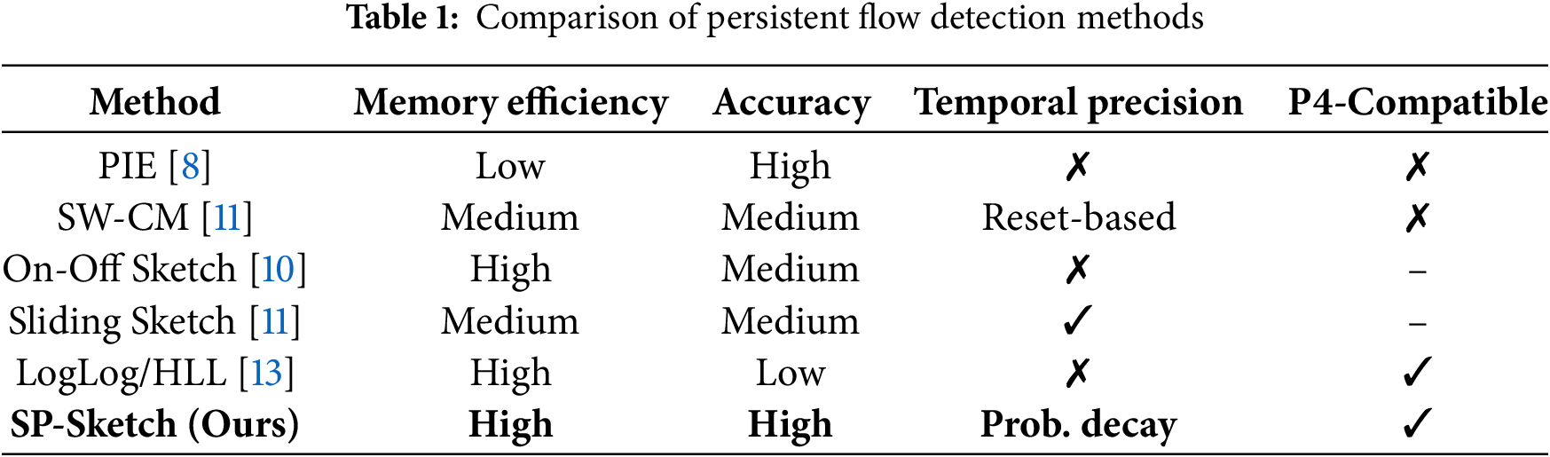
Table 1 compares these persistent flow detection methods in terms of memory efficiency, accuracy, temporal precision, and P4 compatibility. In contrast, SP-Sketch is specifically designed for fine-grained, real-time tracking of individual persistent flows while supporting persistent spread estimation. It integrates probabilistic operations within a single sketch structure, eliminating multiple instances or offline computation. This lightweight approach is compatible with programmable switch constraints, addressing a critical gap in existing methods.

3  Design of SP-Sketch

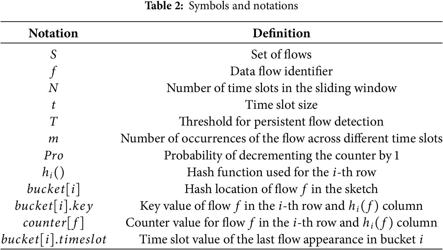
We propose SP-Sketch, a probability-based sliding window sketch designed for efficient persistent flow detection on the programmable data plane. Some key notations that will be used are summarized in Table 2.

3.1 Overview

SP-Sketch is a novel method for persistent flow detection on programmable switches. A flow is defined by its source and destination IP addresses (simplified for clarity; 5-tuple definitions remain valid elsewhere) and is considered persistent if it appears in at least T different time slots within the observation window. The goal of SP-Sketch is to efficiently identify such flows in sliding window scenarios under high-volume traffic with numerous concurrent flows [17].

To minimize memory usage and control plane communication overhead, we employ a Bloom filter [18] to track the first occurrences of flows. A calculated timeslottimeslot timeslot field, derived from packet timestamps, is used to mark each packet with its corresponding time slot. This method reduces unnecessary resets of the Bloom filter and helps mitigate false positives.

SP-Sketch employs a probabilistic mechanism to manage flow counters and approximate the expiration of flow activity in the oldest slot. Instead of creating new sketch structures, SP-Sketch uses probabilistic operations to update the existing counters. This approach simulates the expiration of flow activity without requiring additional memory for new data structures, thus reducing memory consumption and enhancing overall efficiency.

To address the challenge of updating flow counters when packets appear intermittently across time slots, SP-Sketch utilizes a match-action table to store the pre-calculated probability updates for each flow, thereby enabling efficient retrieval and updating of flow counters even when the flow appears in non-continuous slots.

The following subsections present the detailed methodology of SP-Sketch, including its data structures, algorithms, basic operations and the relevant discussion and analysis.

3.2 Data Structure

Data Structure: The data structure of SP-Sketch contains three rows and each row has w buckets, as illustrated in Fig. 2a. Each bucket is divided into three parts. The first part stores a key value (i.e., source IP address and destination IP address). The second part is a counter that tracks the number of slots that this flow occurs within the current time window. The third part is a field named timeslot that records the last appearance of the flow, as mentioned in Section 3.1.

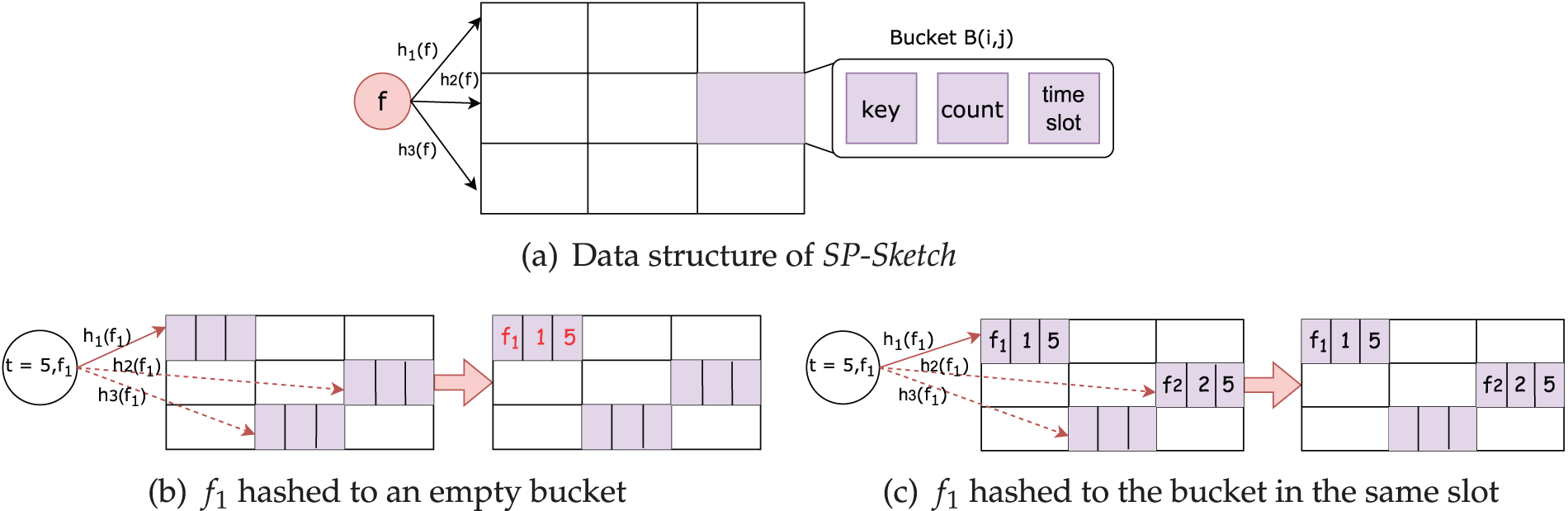
Figure 2: SP-Sketch data structure and the packet’s flow information insertion process. (a) Data structure of SP-Sketch, (b) f1 hashed to an empty bucket, and (c) f1 hashed to the bucket in the same slot

When a data packet arrives, it is processed by applying three different hash functions to map it to three specific buckets within the sketch. The counters associated with these buckets are then incremented to track the number of times the flow appears in different slots.

Initialization: All buckets are set to 0. Prior to the commencement of the detection process, it is necessary to transmit the relevant table entries information to the data plane from the controller.

3.3 The Insertion Operation

When a packet arrives at the switch, its headers are parsed to extract the source and destination IP addresses. These two components are then passed to three distinct hash functions, each generating a hash value. These hash values are used to identify the corresponding buckets in the sketch where the packet’s flow information is stored.

Next, SP-Sketch traverses these three buckets. If the packet’s source IP address and destination IP address match the key (i.e., source IP address and destination IP address) stored in any one of these buckets, the counter of that bucket will be incremented, and the packet is considered successfully inserted. If an empty bucket is encountered and the buckets before the empty bucket do not have matching keys with the packet, the packet’s flow information will be inserted into the empty bucket. Specifically, we set the key to the packet’s source IP address and destination IP address, set the counter value to 1, and set the timeslot to the packet’s timeslot.

If no matching flow is found and all the corresponding buckets are full, the replacement operation is triggered. In this operation, one of the existing flows in the full buckets is evicted to make room for the new flow. The evicted flow is selected based on a probabilistic strategy, which involves factors such as the least recently updated flow or other criteria designed to optimize memory usage. The new flow’s information is then inserted into the selected bucket, replacing the evicted flow’s data.

For example, as shown in Fig. 2b, when the packet belonging to flow f1 arrives at the switch during the fifth slot, all buckets are empty. The packet is inserted into the first available bucket, and the flow’s information, such as bucket[i].count, bucket[i].timeslot, and bucket[i].key, is updated accordingly. If a matching flow is not found and no empty bucket is available, the replacement operation will be triggered to evict an existing flow and insert the new packet into the sketch.

3.4 The Update Operation

The update operation is the core of SP-Sketch that maintains flow persistence tracking across sliding time windows. This section details the four key components of the update process.

3.4.1 Detecting Time Slot Difference

When a data packet arrives, it is hashed to three buckets and checked for corresponding key values. The first step is to compare the current time slot with the slot value corresponding to the key in the sketch. If both slot values are equal, it means that the two packets of the flow appear in the same slot, so no further counting is needed.

As illustrated in Fig. 2c, at the fifth slot, f1 finds the corresponding position, and no operation is performed because it belongs to a flow that repeatedly appears in the same slot. The update operation is only performed when the slot value exceeds the last occurrence, meaning the flow has entered a new slot in the current window.

3.4.2 Calculating Delta

If the packet occurs in a different slot, the system calculates the number of missed slots between the current arrival and the last recorded appearance. The difference between the current time slot and the stored time slot value is recorded as δ, representing the number of time slots that have elapsed since the flow’s last appearance.

This δ value is crucial for determining how many probabilistic decrement operations should be simulated to account for the flow’s absence during the missed slots. The calculation ensures that when a flow appears after multiple slots, the probability is reduced multiple times, not just once.

3.4.3 Determining Decrement Probability

The probabilistic subtraction mechanism adjusts the flow counters based on the appearance of flows across different time slots. When a flow appears in adjacent time slots, the probability of decrementing its counter is given by mN, where m represents the current counter value, and N is the total number of slots in the window.

When a flow reappears after missing Δs slots, we need to simulate the decay that should have occurred during those missed slots. For each missed slot, the decay probability is p=mN where m is the current counter value. The number of decrements k over Δs missed slots follows a binomial distribution: P(k decrements)=(Δsk)pk(1−p)Δs−k. However, since the counter value changes after each decrement, we use the sequential probability: P(final counter=m−k)=∏i=0k−1m−iN⋅∏j=kΔs−1N−(m−j)N.

3.4.4 Performing Probabilistic Update

A random number is generated to determine whether the decrement operation should be performed based on the calculated probability. The corresponding counter value is then read and potentially decremented according to the probabilistic decision.

As illustrated in Fig. 3a, the probabilistic mechanism determines whether a decrement operation occurs when flow packets arrive after missing time slots.

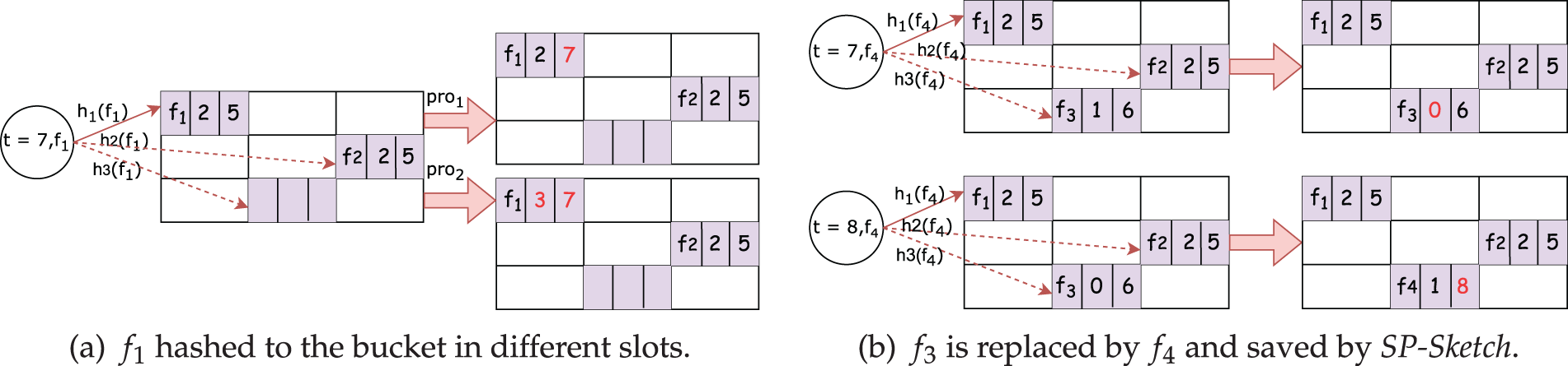
Figure 3: SP-Sketch collision handling and flow replacement mechanism. (a) f1 hashed to the bucket in different slots, and (b) f3 replaced by f4 and saved by SP-Sketch

Fig. 4 provides a comprehensive step-by-step example where flow f1 appears in slots S1, S2, S6, and S8, while being absent during slots S3, S4, S5, and S7. The figure shows how the counter evolves from 0 to 3 across eight time slots. Key observations include: (1) the counter increments by 1 when flow packets arrive in consecutive slots (S1→S2), (2) the counter remains unchanged during absent periods (S3–S5), and (3) probabilistic decrements occur when flows reappear after missing multiple slots, as demonstrated in S6 where Δs=3, P=0.4, and a random value of 0.3 triggers the decrement operation before adding the new packet.

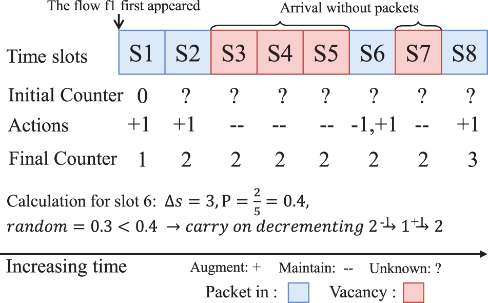
Figure 4: Step-by-step counter update process

Finally, when Δs is greater than or equal to the window size N, the counter is directly set to 0, indicating that the flow has been absent for too long and is no longer part of the current window.

The complete update procedure is formalized in Algorithm 1. The algorithm examines d hashed rows and performs constant-time actions with time complexity 𝒪(d), making it well-suited for the parallel pipeline of programmable switches like Tofino.

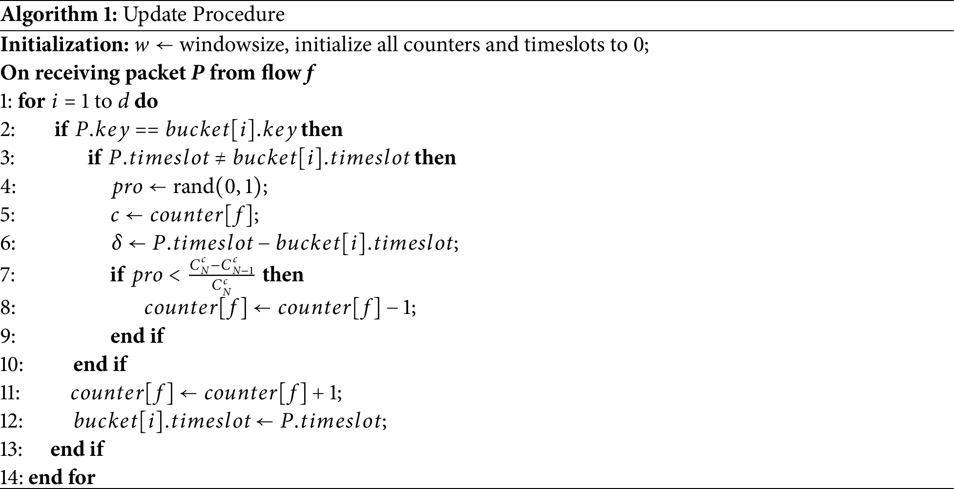
The algorithm uses simplified notation where counter[f] represents the counter value for flow f, and bucket[i] represents the bucket at position i. This notation makes the algorithm more readable while maintaining the same functionality as the original formulation.

3.4.5 Mathematical Foundation and Convergence

Convergence Guarantee: The probabilities satisfy ∑k=0min(m,Δs)P(final counter=m−k)≤1, ensuring mathematical consistency.

Numerical Example: Consider m=3, N=5, Δs=2: P(k=0)=25×25=0.16; P(k=1)=35×35+25×35=0.6; P(k=2)=35×25=0.24. Total: 0.16+0.6+0.24=1.0, confirming perfect convergence. This approach provides equivalent functionality while being mathematically verifiable and computationally efficient. Finally, when Δs is greater than or equal to the window size N, B(i,hi(f)).count is directly set to 0, indicating that the flow has been absent for too long and is no longer part of the current window.

3.5 The Replace Operation

The replace operation handles the hash collisions when multiple flows map to the same bucket locations. This operation consists of three main phases: conflict detection, minimum-count entry identification, and the application of decrement or replacement strategies. This section details each phase to provide a comprehensive understanding of the collision handling mechanism.

3.5.1 Conflict Detection

When a new packet from flow f arrives, the system first attempts to locate the flow in its three hashed bucket positions. If any of these buckets contain a matching key, the packet is processed normally without triggering the replacement operation.

A conflict occurs when all three hashed buckets are occupied by different flows (non-matching keys). At this point, the system must decide which existing flow to potentially evict to make room for the new flow. This conflict detection phase is crucial for maintaining the sketch’s integrity while accommodating new flows under memory constraints.

The conflict detection process checks whether P.key≠B(i,hi(f)).key for all i∈{1,2,3}. Only when this condition is satisfied for all three buckets does the system proceed to the next phase of identifying the minimum-count entry.

3.5.2 Identifying Minimum-Count Entry

Once a conflict is detected, the system identifies the entry with the smallest counter value among the three candidate buckets. This identification process is designed to preserve flows with higher counter values, which are more likely to represent persistent flows.

The minimum-count identification examines the counter values bucket[i].count for each of the three hashed positions and selects the entry with the smallest value. In case of ties, the system selects the first encountered minimum entry. This strategy ensures that flows with stronger persistence indicators (higher counters) are preferentially retained in the sketch.

The selection of the minimum-count entry is performed using simple comparison operations that are well-suited to the constraints of P4 programmable switches, avoiding complex sorting algorithms that would be resource-intensive.

3.5.3 Applying Decrement or Replacement

After identifying the minimum-count entry, the system applies one of two strategies: decrement the counter or perform direct replacement. The choice between these strategies depends on the current counter value and timing conditions.

Decrement Strategy: If the minimum counter value is greater than 0, the system decrements it by 1. This gradual reduction approach allows persistent flows to persist longer in the sketch, as they need multiple collision events to be completely evicted. The decrement operation also considers the time slot difference to ensure proper temporal handling.

Replacement Strategy: When the minimum counter hits 0, direct replacement occurs. The existing flow’s key is replaced with the new flow’s key, and the counter is set to 1. This ensures that completely aged-out flows are efficiently removed to make room for new active flows.

3.5.4 Simplified Replace Algorithm

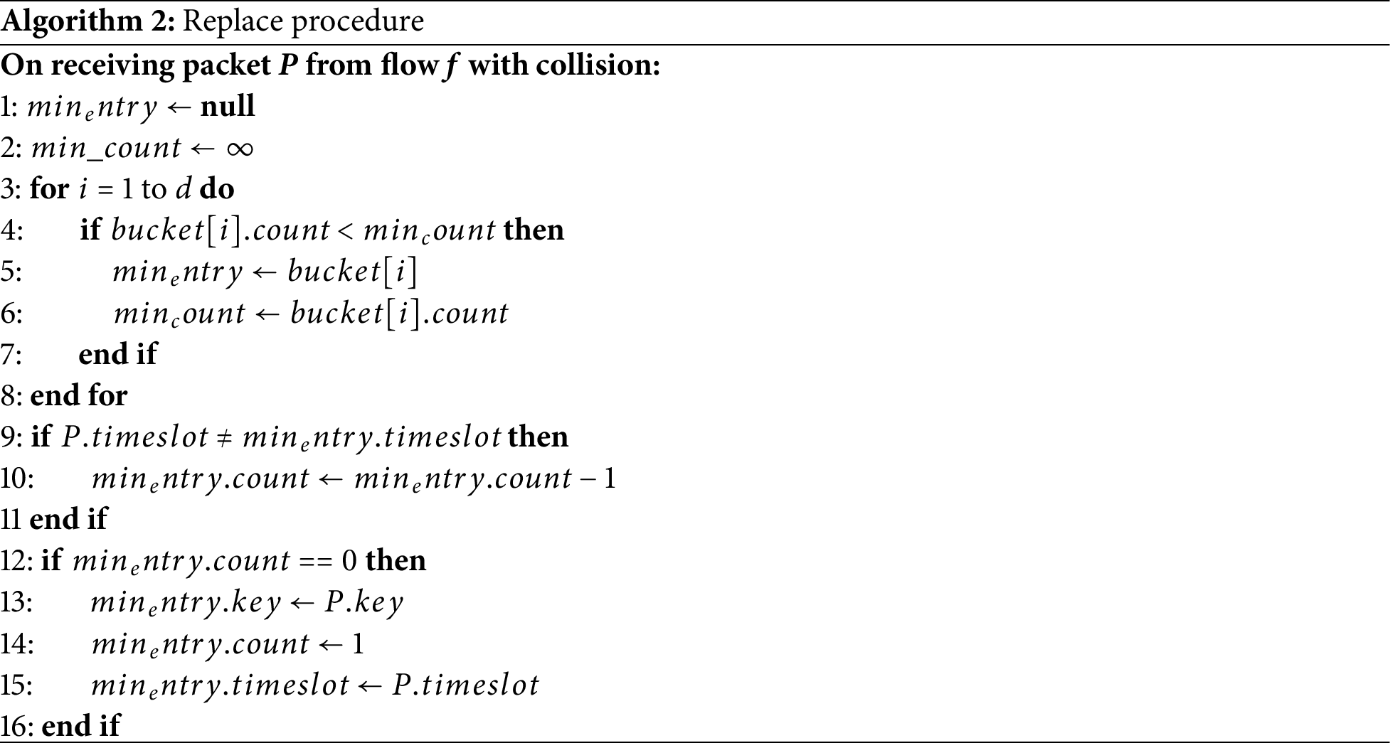
The complete replace procedure is formalized in Algorithm 2. The algorithm eliminates nested loops and uses a streamlined approach for better efficiency and readability.

3.5.5 Decision Flow for Decrement vs. Replacement

The decision process for applying decrement or replacement follows a clear decision tree structure: The application of decrement or replacement is guided by a structured decision tree, depicted in Fig. 5. Upon packet arrival, the system checks for conflicts across three hashed buckets to ascertain flow occupancy. If no conflict arises, processing proceeds as usual. Upon conflict detection, the system selects the bucket with the lowest count. Actions depend on the minimum count: a decrement triggers a complete eviction check (counter == 0); immediate replacement occurs if the count is already zero. This method ensures efficient memory use and maintains flows with higher persistence.

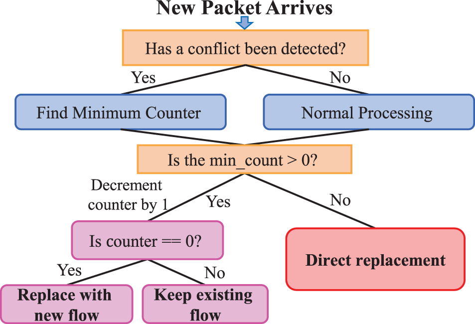
Figure 5: A decision tree diagram of replacement

3.6 The Query Operation

Based on the aforementioned operations, the objective is to maximize the retention of persistent flows within the most recent window in the sketch structure. During querying, it is only necessary to traverse all registers to identify the key value associated with a flow whose counter value surpasses the slot threshold. This scan has time complexity 𝒪(d⋅w), where d is the number of hash rows and w is the number of entries per row. Although linear in sketch size, it is invoked periodically and can be offloaded or parallelized on the switch’s control processor.

Overall, the sliding window probability reduction method provides a more accurate and reliable approach to detecting persistent flows in real-time network traffic monitoring. By accounting for the sliding window technique and the probabilistic nature of persistent flows, this method helps minimize errors and improve the accuracy of network traffic analysis.

3.7 Discussion and Analysis

3.7.1 Flow Persistence Estimation

We first derive the expected value of flow persistence P, which is defined as the number of distinct time intervals in which a flow appears within the sliding window. Let N be the total number of time intervals, v the number of intervals in which the flow appears, and θ the probability of the flow appearing in any given interval. We aim to calculate E(P), the expected average persistence of the flow across multiple time windows, using a binomial distribution.

Step 1: Computing the Probability Distribution of P

Suppose a flow appears in v distinct time intervals. The probability of this event follows a binomial distribution. The binomial distribution describes the number of successes in a fixed number of independent trials. In this case, each time interval can be considered a trial, and the appearance of the flow in that time interval counts as a success.

The probability that the flow appears in exactly v time intervals is given by: P(P=v)=(Nv)⋅θv⋅ (1−θ)N−v. As described earlier, (Nv) represents the number of ways to choose v intervals from N total intervals, and the terms θv and (1−θ)N−v represent the probability of the flow appearing in v intervals and not appearing in the remaining N−v intervals, respectively.

Step 2: Computing the Expected Value E(P)

The expected value E(P) is a statistical measure representing the average persistence of a flow. According to probability theory, the expected value can be computed by multiplying each possible value of v by its corresponding probability and summing over all possible values of v: E(P)=∑v=0Nv⋅(Nv)⋅θv⋅(1−θ)N−v.

As previously defined, v represents the possible values of persistence P, and (Nv) is the combination term representing the number of ways to choose v intervals from N. The terms θv⋅(1−θ)N−v represent the probability of the flow appearing in exactly v time intervals.

3.7.2 Fairness of Replacement Strategy

In SP-Sketch, the replacement mechanism selects the entry with the smallest counter value among d candidate buckets when a flow collision occurs. This strategy is designed to favor flows with high recent activity, which are more likely to represent high-bandwidth or volumetric behaviors. Such prioritization improves detection accuracy under tight memory constraints by preserving frequent flows that are assumed to be more significant.

However, this approach may introduce a potential fairness issue: low-frequency but long-lived persistent flows can be prematurely evicted if their counters remain small. This is particularly relevant in use cases such as stealthy long-term threat detection or low-rate anomaly monitoring, where such flows may be of high importance despite low volume.

To mitigate this, one possible extension is to incorporate temporal persistence indicators into the replacement strategy, such as exponential aging of counters or incorporating timestamps to track recent activity intervals. Another promising direction is to explore hybrid replacement schemes (e.g., combining count with time decay or using reservoir sampling) to balance between frequency and longevity. We leave the implementation of these advanced strategies to future work.

3.7.3 Fairness Analysis of Decay Mechanism

A critical concern in SP-Sketch is whether the packet-driven decay mechanism ensures consistent counter decay rates across all flows. We provide a rigorous mathematical analysis proving that while instantaneous fairness may vary, the system achieves statistical fairness in expectation.

Theorem 1 (Expected Decay Rate Consistency): In SP-Sketch, all flows achieve consistent expected decay rates under appropriate conditions.

Proof: Let flow fi have packet arrival rate λi (packets per slot) and counter value Ci(t) at time slot t. The packet arrivals follow a Poisson process, so the probability of k packet arrivals in slot Δt is: P(Ni=k)=(λiΔt)ke−λiΔtk!. Given k packet arrivals, the probability of at least one decay operation is: P(decay|Ni=k)=1−(1−Ci(t)N)k. The expected decay probability becomes: E[Pdecay,i]=∑k=0∞P(decay|Ni=k)⋅P(Ni=k) =1−e−λiΔt∑k=0∞(1−Ci(t)N)k(λiΔt)kk!=1−e−λiΔtCi(t)N.

When λiΔtCi(t)N≪1 (typical in practice), using Taylor expansion: E[Pdecay,i]≈λiΔtCi(t)N. This shows the expected decay rate is proportional to the target rate Ci(t)N with factor λiΔt. ◻

Theorem 2 (Error Bounds): The relative error in decay rates is bounded and predictable.

Proof: The relative error is defined as: ϵi=|E[Pdecay,i]−Ci(t)N|Ci(t)N=|N(1−e−λiΔtCi(t)N)Ci(t)−1|. For the critical case λiΔt=1 (one packet per slot): ϵi=|N(1−e−Ci(t)N)Ci(t)−1|≈0 when Ci(t)N≪1. In general, the error is bounded by: ϵi≤max(|λiΔt−1|,1λiΔt−1). This bound approaches zero as λiΔt→1. ◻

Theorem 3 (Long-Term Stability): Cumulative errors remain bounded over multiple time slots.

Proof: Let Ei(T) be the cumulative error over T slots. Since each slot’s error is bounded by ϵmax, we have |Ei(T)|T≤ϵmax=O(1). Due to natural counter bounds (0≤Ci(t)≤N), the long-term average error remains finite and does not diverge. ◻

Practical Implications: This analysis establishes that: (1) Perfect statistical fairness is achievable when flows have approximately one packet in each slot; (2) Deviation errors are bounded and predictable; (3) For typical network traffic where most flows have moderate packet rates (λiΔt∈[0.5,2]), the relative error remains below 10%; (4) The system maintains long-term stability without error accumulation.

3.7.4 Hash Collision Impact on Decay Accuracy

Hash collisions affect SP-Sketch decay accuracy since the decay probability mN depends on counter values that may be distorted by multiple flows mapping to the same bucket. We provide theoretical analyses of the collision-error relationship and mitigation strategies.

Collision-Error Relationship: When bucket j has collision set 𝒞j with flows {m1,m2,...,mk}, the counter m^j differs from individual persistence mi, causing a decay error. The collision probability is Pcollision≤1−e−n22w and the expected error is E[ϵcollision]≤nw⋅N−1N. For a typical load factor α≤0.7, the collision error remains below 7%.

Collision Mitigation Strategies: SP-Sketch employs several design principles to minimize hash collision impact: (1) Multi-hash verification: Using d=3 independent hash functions reduces the collision probability from nw to (nw)3; (2) Hash function independence: CRC32 with different seeds ensures statistical independence; (3) Counter-based replacement: The minimum-counter replacement strategy preserves persistent flows with higher accuracy; (4) Load factor control: Maintaining α<0.7 keeps the collision probability manageable. These strategies ensure the collision impact remains bounded and predictable.

3.7.5 Error Analysis

In this section, we analyze the error in the persistence estimation used by SP-Sketch. Let Pt(ei) and Pt(ei)^ represent the true and estimated persistence of flow ei in the t-th time interval, respectively. The error term for the minimum persistence in the t-th interval is denoted by ct, and l is the first time interval in which flow ei is inserted into the sketch. Additionally, q is the number of additional intervals between l and t in which flow ei appears.

Step 1: Estimation error when a replacement operation is triggered

When flow ei is not found in the bucket during the query process, the estimated persistence is set to 0. Therefore, the error is 0 in this case.

If flow ei is already stored in the bucket, there are two possible cases:

•   Case 1: Flow ei does not require replacement, meaning its estimated persistence Pt(ei)^ is equal to its true persistence Pt(ei). In this case, the estimation error is 0.

•   Case 2: Flow ei is replaced by another flow. Suppose flow ei arrives at the l-th time interval, and the minimum persistence in the bucket is cl−1. In this case, the estimated persistence of flow ei at time interval l is: Pl(ei)^=cl−1+1.

Step 2: Inductive derivation of the estimation error bound

We now proceed to derive the relationship between the estimated persistence and the true persistence of the flow using mathematical induction.

Base case: When the flow ei is not found in the bucket at time interval t, the estimated persistence is set to 0, i.e., Pt(ei)^=0. Therefore, the error in this case is 0, which satisfies the error bound Pt(ei)^≤Pt(ei)+ct, since ct=0.

Inductive hypothesis: Assume that for time interval l, the flow ei has been inserted into the sketch, and the persistence estimate at time interval l is Pl(ei)^=cl−1+1. We will show that for time interval t, the estimated persistence is bounded by the true persistence and the error term.

Inductive step: Suppose flow ei appears q additional times between intervals l and t, with q≤Pt(ei)−1. The estimated persistence at time t is: Pt(ei)^=Pl(ei)^+q=cl−1+1+q≤cl−1+Pt(ei).

This shows that the estimated persistence Pt(ei)^ is bounded by the true persistence Pt(ei) plus the error term cl−1. Therefore, the error is bounded by: Pt(ei)^≤Pt(ei)+ct, where ct is the error term for the minimum persistence in the t-th interval.

Summary of the error bound: The key formula that represents the relationship between the estimated persistence Pt(ei)^ and the true persistence Pt(ei) is as follows:

Pt(ei)^=Pl(ei)^+q≤cl−1+1+Pt(ei)−1=cl−1+Pt(ei)≤Pt(ei)+ct.(1)

This formula captures the progression of the estimated persistence from time interval l to t, showing that the error is bounded by ct, thereby ensuring the accuracy of the SP-Sketch algorithm within a predictable error range.

4  Implementation on P4 Programmable Switches

We have implemented a prototype of SP-Sketch on P4 hardware switches with Intel Tofino ASIC. SP-Sketch uses CRC32 as the hash function. The Tofino switch operates in a packet-driven manner during the sliding window process. As shown in Fig. 6, probability table entries are transmitted from the controller to the data plane before the detection process begins. If no packet arrives within a time slot, the flow information remains unchanged.

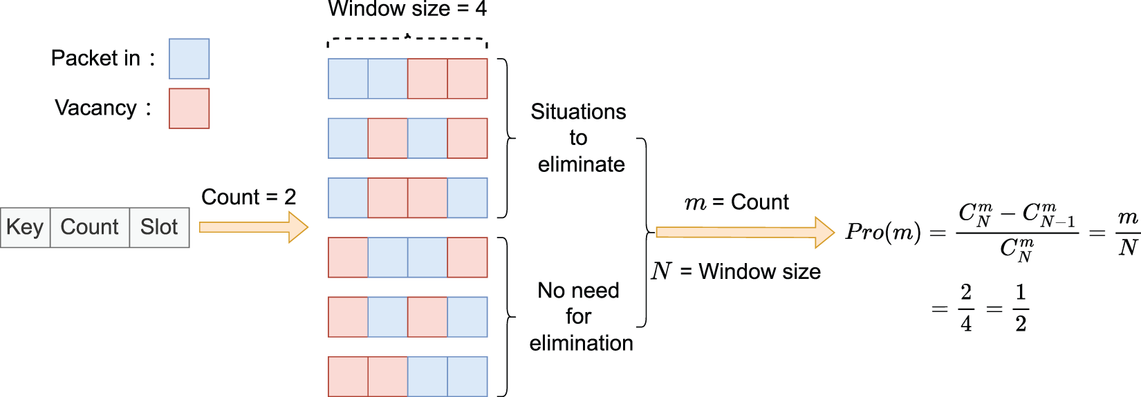
Figure 6: Probability subtraction algorithm flow of SP-Sketch

To handle the sliding window, SP-Sketch computes the delta value, which indicates the movement of the window by subtracting the current packet’s slot value from the sketch’s corresponding value. Since P4 switches do not support floating-point operations, probability updates are simulated using integer slot ranges, and a random number generator determines the probability based on the range.

Flow information, including the flow’s key, counter, and timestamp, is stored in the registers. The window slides forward when a packet’s timestamp exceeds the stored value, and the flow’s count is updated based on the calculated delta. This mechanism helps efficiently track flow activity while meeting the resource constraints of the Tofino switch.

5  Experiment

5.1 Experimental Setup

We have evaluated SP-Sketch using both P4 hardware switches (with Intel Tofino ASIC) and software switches (i.e., BMv2). A flow is considered to be persistent if it appears in at least T=5 distinct timeslots, where T is the persistence threshold.

Dataset: Two public datasets are used to evaluate the efficiency and accuracy of SP-Sketch in detecting persistent flows under both attack and real traffic scenarios:

•   Datacenter: This dataset consists of real internet traffic traces collected by CAIDA’s passive monitors from the “equinix-nyc” location in 2023 [19]. The dataset includes approximately 2 million packets and 64,127 distinct flows identified by source IP (srcIP), making it a valuable source for testing SP-Sketch’s performance in real-world network conditions.

•   DDoS: This dataset consists of simulated malicious traffic (normal and attack packets) to evaluate SP-Sketch’s performance in persistent flow detection under adverse conditions. This dataset is sourced from Sharafaldin et al. [20], which includes a variety of attack scenarios to mimic real-world DDoS activities.

Evaluation Metrics:

•   Average Relative Error (ARE): 1n∑i=1n|yi^−yi|yi, where yi is the real persistence of flow fi, yi^ is the estimated persistence, and n is the size of the query set. The query set comprises the reported flows whose persistence is higher than a predefined threshold.

•   Mean Squared Error (MSE): 1n∑i=1n(yi^−yi)2, where yi is the real persistence of flow fi, yi^ is the estimated persistence, and n is the query set. The MSE serves as a metric to quantify error. A smaller MSE value, approaching zero, signifies a reduction in error magnitude at the corresponding time point.

•   Precision Rate (PR):Precision measures the proportion of true positives (TP) among all instances predicted as positive (TP + FP), where TP refers to true positives and FP refers to false positives. It is defined as: PR=TPTP+FP.

•   Recall Rate (RR): Recall, also known as sensitivity, measures the proportion of true positives (TP) that are correctly identified among all actual positives (TP + FN), where FN refers to false negatives. It is defined as: RR=TPTP+FN.

•   Throughput: Throughput measures the amount of data or packets processed per unit of time. In the experiment, it is evaluated using the tool iperf and is defined as the number of packets or bits processed per second, i.e., Throughput=Total Data ProcessedTime Taken. The “Total Data Processed” is in bytes or bits, and “Time Taken” is in seconds.

5.2 Experimental Results

Fig. 7 shows how precision vaires with memory (512 to 32,768 KB) and window sizes (1–64 t) under 25 and 100 Mbps loads. Medium load (25 Mbps) achieves higher precision than high load (100 Mbps), with both showing increasing but diminishing improvement as memory and window size grow. Error bars indicate stable estimates, though high load shows greater variability.

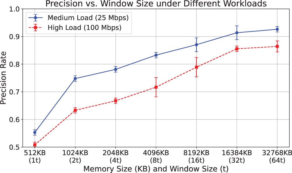
Figure 7: Precision vs. window size under different workloads

Fig. 8a reveals the ARE of different methods under the datacenter dataset. The horizontal axis denotes slot size characterized by parameter “t” (approximately 2 s duration). SP-Sketch maintains consistently low ARE regardless of slot span size, indicating minimal difference between estimated and actual values. When slot duration reaches 8 t, SP-Sketch achieves an ARE of approximately 0.1, while PI-Sketch reaches 0.137 and the SW-CM method (sliding window [11] plus count-min sketch [21]) escalates to around 0.18. As slot duration expands to accommodate more data, ARE tends to rise across all methods. The same pattern appears in Fig. 8b under DDoS conditions. Although ARE increases with slot size in all methods, SP-Sketch demonstrates slower growth due to its probabilistic subtraction mechanism enabling smooth state decay without resetting multiple sketch instances, thereby mitigating error and maintaining greater stability.

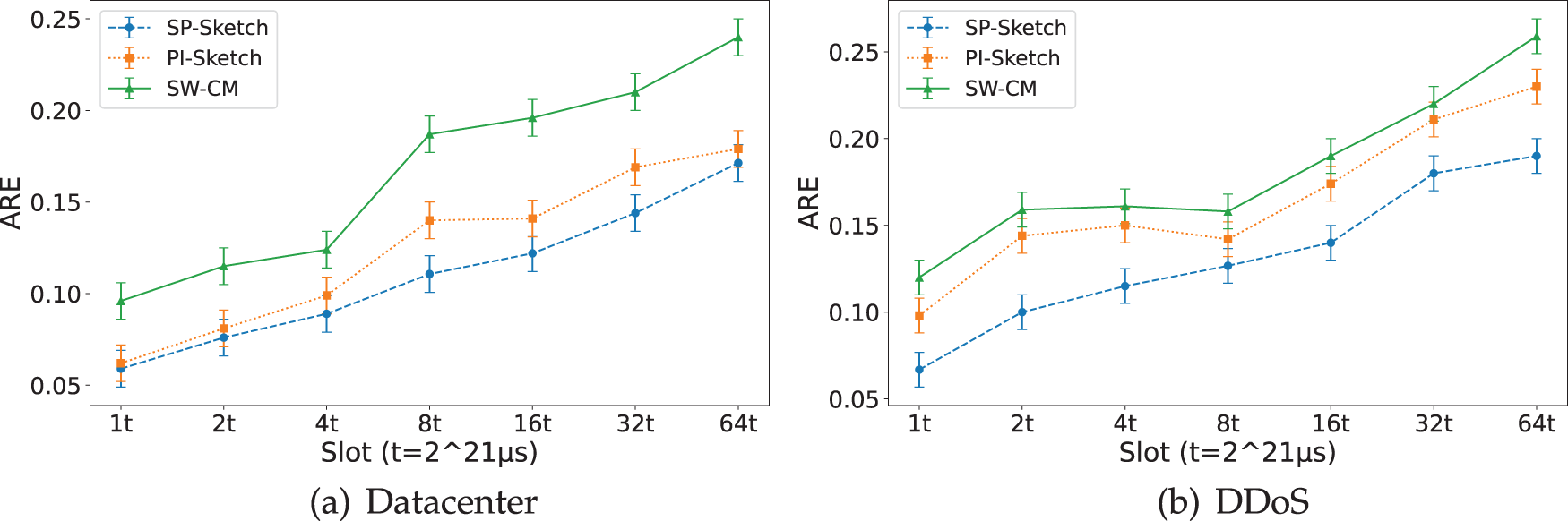
Figure 8: ARE of different datasets under different slot span sizes. (a) Datacenter (b) DDoS

As demonstrated in Fig. 9a, when the slot span is small, the precision rate exhibits a high value, although it does not reach the same level of precision as the other two methods. This initial performance characteristic may be attributed to probabilistic initialization effects. The baseline method (SW-CM) lacks consideration for situations involving hash collisions and their subsequent replacement. Consequently, when the slot span becomes relatively large, specifically when the slot time extends to two minutes, its effectiveness diminishes substantially. In Fig. 9b, within the DDoS dataset, the PI and SP-Sketch methods exhibit comparable levels of accuracy, and both consistently outperform the baseline method. However, as the slot span surpasses 16 seconds, SP-Sketch consistently maintains a marginally superior level of accuracy compared to PI.

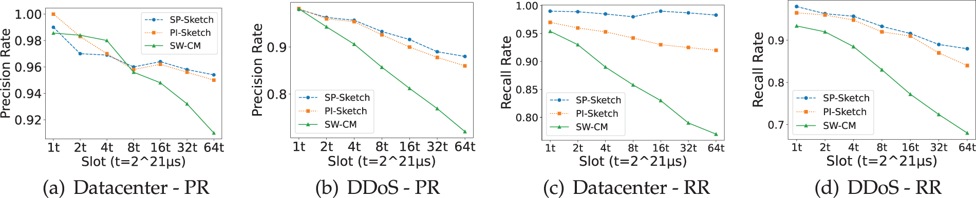
Figure 9: PR and RR of different datasets under different slot span sizes. (a) Datacenter-PR (b) DDoS-PR (c) Datacenter-RR (d) DDoS-RR

The PR and RR exhibit an interdependent relationship: emphasizing high precision typically reduces recall, while prioritizing recall often compromises precision. Given the context of persistent flow detection, a balance is sought between comprehensiveness and precision. Efforts focus on maximizing recall while maintaining specified precision levels.

Fig. 9c,d shows that the sliding window method primarily addresses false negatives from fixed-time interval detection. Consequently, this method achieves significantly higher recall than the other two methods, approaching 1. This advantage is especially pronounced when dealing with fewer persistent flows, making detection more efficient. For instance, as shown in Fig. 9c, the data center environment exhibits a remarkably high RR of 98.7%.

5.3 Evaluation on P4 Hardware Switches with Tofino ASIC

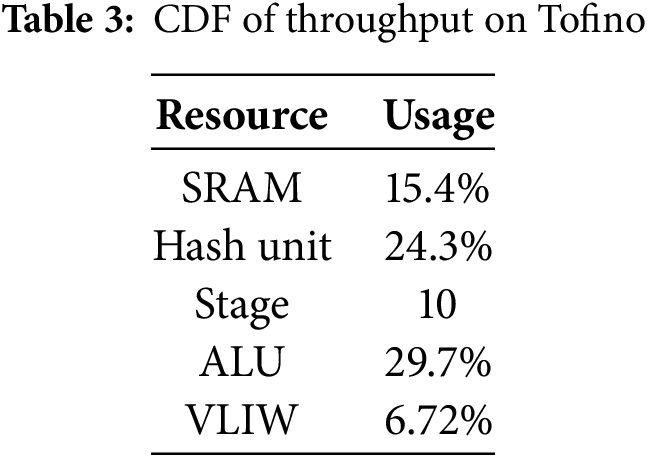
To evaluate SP-Sketch performance in real-world scenarios, we implemented it on P4 hardware switches with Intel Tofino ASIC. This platform was selected for its high throughput and comprehensive programmability, making it well-suited for persistent flow detection in high-speed networks. Resource utilization on the P4 hardware switch is shown in Table 3. The ALU and Hash units are the most heavily utilized resources, consuming 29.7% and 24.3% of total capacity.

To evaluate practicality, we measured the throughput of SP-Sketch on a Tofino switch using a 10 Gbps optical fiber interface. As shown in Fig. 10, SP-Sketch achieves an average of 9.5 Gbps, close to line rate. Compared to PI-Sketch with similar throughput, SP-Sketch additionally offers real-time sliding-window detection with better temporal precision.

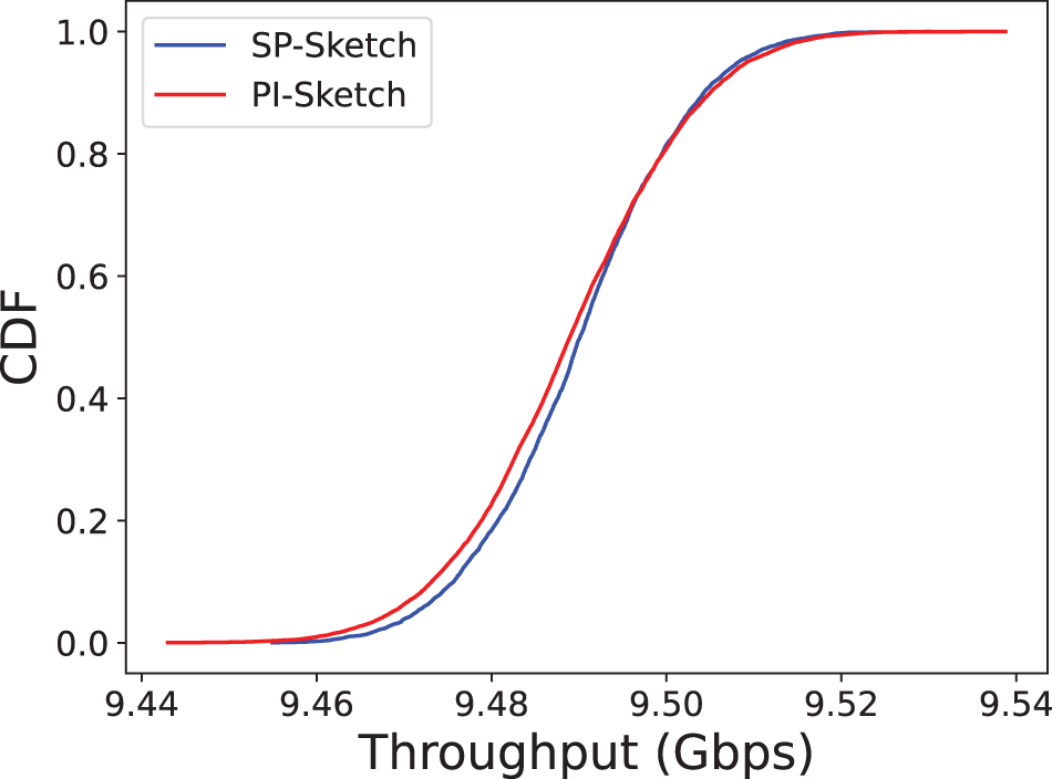
Figure 10: Resource usage of Tofino

5.4 Use Case: Detecting Persistent Heavy Changes

In this experiment, we assess the performance of SP-Sketch in detecting Persistent Heavy Changes (PHC). As the slot size increases, the error in SP-Sketch increases, but even when the slot size is increased sixfold, both ARE and MSE remain relatively low. For instance, in the Datacenter scenario (i.e., Fig. 11a, b), when the slot size is 8 t, the ARE is below 0.1 and MSE is below 2. The error is mostly concentrated in the first stage, with a more pronounced cumulative effect in later stages. Fig. 11 demonstrates that while SP-Sketch’s error increases with slot size, it still outperforms traditional methods, maintaining low error rates and high accuracy.

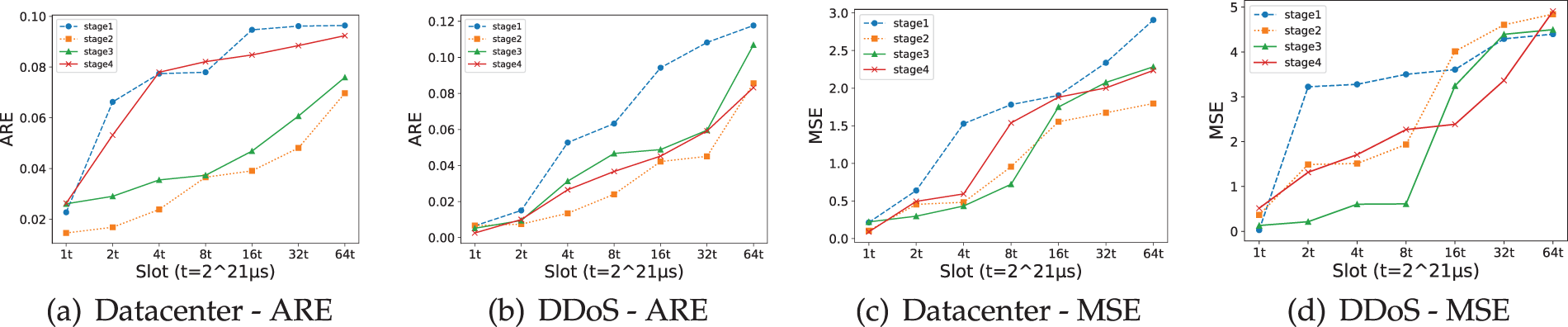
Figure 11: ARE and MSE performance of SP-Sketch under different slot sizes. (a) Datacenter-ARE (b) DDoS-ARE (c) Datacenter-MSE (d) DDoS-MSE

6  Conclusion

In this paper, we introduce SP-Sketch, a novel sliding-window-based approach for persistent flow detection in real-time applications on programmable data planes. SP-Sketch leverages a probabilistic subtraction mechanism to simulate slot expiration, substantially reducing memory consumption while preserving high accuracy. Contrasting traditional methods that necessitate multiple sketch instances or timestamp storage, SP-Sketch adopts for a single sketch structure, enhancing memory efficiency. We conduct an analysis of SP-Sketch’s error bounds, demonstrating its effectiveness in practical settings. Our implementation on Intel Tofino hardware and BMv2 software switches demonstrates its practicality and efficiency. Experimental results indicate that SP-Sketch boosts accuracy by up to 20% and recall by 5% compared to non-sliding methods, positioning it as a robust and memory-efficient solution for real-time persistent flow detection in high-speed network environments.

Acknowledgement: Not applicable.

Funding Statement: This work was supported by the National Undergraduate Innovation and Entrepreneurship Training Program of China (Project No. 202510559076) at Jinan University, a nationwide initiative administered by the Ministry of Education, and the National Natural Science Foundation of China (NSFC) under Grant No. 62172189.

Author Contributions: The authors confirm contribution to the paper as follows: Conceptualization, Yuqian Huang, Luyi Chen and Lin Cui; methodology, Yuqian Huang and Luyi Chen; software, Yuqian Huang and Luyi Chen; validation, Yuqian Huang, Luyi Chen and Zilun Peng; formal analysis, Yuqian Huang and Luyi Chen; investigation, Yuqian Huang and Luyi Chen; resources, Lin Cui; data curation, Yuqian Huang and Luyi Chen; writing—original draft preparation, Yuqian Huang; writing—review and editing, Yuqian Huang, Luyi Chen and Lin Cui; visualization, Yuqian Huang and Luyi Chen; supervision, Lin Cui; funding acquisition, Lin Cui. All authors reviewed the results and approved the final version of the manuscript.

Availability of Data and Materials: The authors confirm that the data supporting the findings of this study are available within the article.

Ethics Approval: Not applicable.

Conflicts of Interest: The authors declare no conflicts of interest to report regarding the present study.

References

1. Liu B, Tang D, Chen J, Liang W, Liu Y, Yang Q. ERT-EDR: online defense framework for TCP-targeted LDoS attacks in SDN. Expert Syst Appl. 2024;254(1):124356. doi:10.1016/j.eswa.2024.124356. [Google Scholar] [CrossRef]

2. León A, Perdices D, García-Dorado JL, Ramos J, Aracil J. An expert-aware Markovian system for end-user proactive troubleshooting in the Network and Security Operations Center. Expert Syst Appl. 2025;276(1):127072. doi:10.1016/j.eswa.2025.127072. [Google Scholar] [CrossRef]

3. Singamaneni Krishnapriya SS. A comprehensive survey on advanced persistent threat (APT) detection Techniques. Comput Mater Contin. 2024;80(2):2675–719. doi:10.32604/cmc.2024.052447. [Google Scholar] [CrossRef]

4. Narmadha S, Balaji N. Improved network anomaly detection system using optimized autoencoder-LSTM. Expert Syst Appl. 2025;273(9):126854. doi:10.1016/j.eswa.2025.126854. [Google Scholar] [CrossRef]

5. Gou X, Zhang Y, Hu Z, He L, Wang K, Liu X, et al. A sketch framework for approximate data stream processing in sliding windows. IEEE Transact Know Data Eng. 2023;35(5):4411–24. doi:10.1109/tkde.2022.3151140. [Google Scholar] [CrossRef]

6. Zhang X, Cui L, Tso FP, Deng Y, Li Z, Jia W. Monte: SFCs migration scheme in the distributed programmable data plane. IEEE Transact Parallel Distrib Syst. 2025;36(4):633–44. doi:10.1109/tpds.2025.3532467. [Google Scholar] [CrossRef]

7. Zhang X, Cui L, Lau W, Tso FP, Deng Y, Jia W. Carlo: cross-plane collaboration for multiple in-network computing applications. In: IEEE Conference on Computer Communications (INFOCOM); 2024 May 20–23; Vancouver, BC, Canada. p. 1–9. [Google Scholar]

8. Dai H, Shahzad M, Liu AX, Li M, Zhong Y, Chen G. Identifying and estimating persistent items in data streams. IEEE/ACM Transact Netw. 2018;26(6):2429–42. doi:10.1109/tnet.2018.2865125. [Google Scholar] [CrossRef]

9. Dai H, Li M, Liu AX, Zheng J, Chen G. Finding persistent items in distributed datasets. IEEE/ACM Transact Netw. 2019;28(1):1–14. [Google Scholar]

10. Zhang Y, Li J, Lei Y, Yang T, Cui B. On-off sketch: a fast and accurate sketch on persistence. Proc VLDB Endow. 2020;14(2):128–40. doi:10.14778/3425879.3425884. [Google Scholar] [CrossRef]

11. Gou X, He L, Zhang Y, Wang K, Liu X, Yang T, et al. Sliding sketches: a framework using time zones for data stream processing in sliding windows. In: Proceedings of ACM International Conference on Knowledge Discovery & Data Mining (SIGKDD); 2020 Jul 6–10; New York, NY, USA. p. 1015–25. [Google Scholar]

12. Durand M, Flajolet P. Loglog counting of large cardinalities. In: Algorithms-ESA 2003: 11th Annual European Symposium. Springer; 2003 Sep 16–19; Budapest, Hungary. p. 605–17. [Google Scholar]

13. Flajolet P, Fusy É, Gandouet O, Meunier F. Hyperloglog: the analysis of a near-optimal cardinality estimation algorithm. In: 2007 Discrete Mathematics and Theoretical Computer Science (DMTCS); 2007 Jun 17–22; Nancy, France. p. 127–46. doi:10.46298/dmtcs.3545. [Google Scholar] [CrossRef]

14. Xiao Q, Qiao Y, Zhen M, Chen S. Estimating the persistent spreads in high-speed networks. In: 2014 IEEE 22nd International Conference on Network Protocols; 2014 Oct 21–24; Raleigh, NC, USA. p. 131–42. [Google Scholar]

15. Huang H, Sun YE, Ma C, Chen S, Zhou Y, Yang W, et al. An efficient k-persistent spread estimator for traffic measurement in high-speed networks. IEEE/ACM Transact Netw. 2020;28(4):1463–76. doi:10.1109/tnet.2020.2982003. [Google Scholar] [CrossRef]

16. Zhou Y, Zhou Y, Chen M, Chen S. Persistent spread measurement for big network data based on register intersection. Proc ACM on Measur Analy Comput Syst. 2017;1(1):1–29. doi:10.1145/3084452. [Google Scholar] [CrossRef]

17. Chen Y, Wang L, Wang J, Liu S, He K, Wang J, et al. Marlin: enabling high-throughput congestion control testing in large-scale networks. In: EuroSys’25: Proceedings of the Twentieth European Conference on Computer Systems; 2025 Mar 30–Apr 3; Rotterdam, Netherlands. p. 460–74. [Google Scholar]

18. Dong F, Wang P, Li R, Cui X, Zhao J, Tao J, et al. Poisoning attacks and defenses to learned bloom filters for malicious URL detection. IEEE Trans Dependable Secure Comput. 2025;22(4):3275–88. doi:10.1109/tdsc.2025.3528993. [Google Scholar] [CrossRef]

19. CAIDA. Statistical information for the CAIDA Anonymized Internet Traces; 2023 [Internet]. [cited 2025 Apr 13]. Available from: https://www.caida.org/data/passive/passive_trace_statistics. [Google Scholar]

20. Sharafaldin I, Lashkari AH, Ghorbani AA. Toward generating a new intrusion detection dataset and intrusion traffic characterization. In: Proceedings of International Conference on Information Systems Security and Privacy (ICISSP 2018); 2018 Jan 22–24; Madeira, Portugal. p. 108–16. [Google Scholar]

21. Cormode G, Muthukrishnan S. An improved data stream summary: the count-min sketch and its applications. J Algor. 2005;55(1):58–75. doi:10.1016/j.jalgor.2003.12.001. [Google Scholar] [CrossRef]