Hierarchical Mixed-Effects and Stacked Machine Learning Ensembles with Data Augmentation for Leakage-Safe E-Waste Forecasting

1  Introduction

Global e-waste volumes are increasing rapidly, while national reporting remains heterogeneous and often sparse. As a result, national e-waste indicators are a critical but noisy input in capacity planning and the monitoring of collection performance [1,2]. Recent global estimates indicate continued growth through 2030 [3,4]. This surge is driven by higher levels of digital adoption, faster product replacement cycles, shorter device lifespans, and limited repair options. Addressing the e-waste challenge is an important issue in waste management and environmental protection. Improper disposal and unregulated recycling frequently lead to the release of toxic chemicals such as heavy metals and persistent organic pollutants, which can damage ecosystems and human health. Although there are international laws like the EU Waste Electrical and Electronic Equipment (WEEE) Directive and the Basel Convention, a lot of e-waste is not monitored; it’s either exported to another country or processed in an unregulated manner. These data gaps highlight the necessity of developing robust forecasting tools for planning sustainable infrastructure, boosting recycling technology design, and improving compliance with international regulations [5–7].

However, a “small data” paradox exists: most countries have only a dozen annual observations or fewer, so year-ahead forecasts must be learned from short, noisy national histories. In this setting, common machine learning methodologies such as random train–test splits and k-fold cross-validation can lead to misleadingly high accuracy since future information inadvertently leaks into the training set. This inflates the performance metrics far above what can be achieved in genuinely unseen years. Traditional tools to predict e-waste, such as linear regression, autoregressive models, and time-series extrapolation, are often inadequate for modelling the mixed and shifting profiles of e-waste flows. There are many models that presume homogeneity and do not account for variation across regions or through time; generalizing e-waste across countries may be problematic. Models based on previous data are also ineffective when new trends or little information is available. Previously, it has been noted how these standard methodologies are neither flexible nor reliable in such environments.

Recent predictions of e-waste highlight the tension between perceived statistical goodness and actual predictive robustness. This has led to an increasing interest in blending statistical techniques with the versatility of machine learning. The focus of these hybrid methodologies is to balance interpretability against prediction ability. This paper presents a new and flexible forecasting approach to address these limitations. It relies on hierarchical mixed effects models, novel approaches for constructing temporal features, and structured data augmentation [8,9]. Very high R2 values reported on short panels can be misleading when the evaluation is not strictly prospective. If the train–test split or feature construction allows a look-ahead (directly or indirectly), the performance estimates can be inflated relative to true year-ahead generalization on future years. Accordingly, we treat leakage-safe prospective validation as the primary criterion for assessing forecasting reliability in sparse national panels.

In this paper, we recast methodological rigor in e-waste forecasting in terms of the integrity of the temporal split rather than the in-sample fit. To mitigate such leakage issues, we propose a leakage-safe evaluation framework for national-scale e-waste forecasting by using a prospective temporal validation design, training on data from 2005–2016 and reserving 2017–2018 as held-out future data across multiple countries. In this context, we stress-test three modeling paradigms commonly used for small environmental panels: (i) local time-series baselines, (ii) hierarchical mixed-effects models, and (iii) pooled machine learning (ML)/stacking ensembles. These choices are motivated by prior e-waste forecasting and the short-panel evaluation literature, as reviewed in Section 2.

Data scarcity can be partially mitigated through augmentation, but in time-dependent settings, augmentation must preserve the temporal structure to avoid distorting the learning signal. We therefore evaluate a time-series-respecting resampling approach (moving-block bootstrap) as a practical mechanism for increasing effective training diversity under short annual panels, alongside controlled comparisons across modeling families under the same leakage-safe validation design.

The key contributions of this work are:

•   We formulate national e-waste forecasting from sparse annual multi-country panels as a leakage-aware one-step-ahead prediction problem and evaluate the models using a strict prospective split.

•   We provide a controlled empirical comparison of local time-series baselines, hierarchical mixed-effects models, and pooled ML/stacking ensembles under the same information set and validation design.

•   We evaluate moving-block bootstrap augmentation for short panels and report ablations showing when augmentation improves or degrades prospective performance.

•   We quantify the marginal value of feature design, ensembling, and augmentation under leakage-safe prospective evaluation.

This paper is organized as follows: Section 2 reviews related work and positions the research gap. Section 3 describes the data, feature construction, and leakage-safe evaluation design. Section 4 presents the experimental results and ablation studies. Section 5 concludes with the limitations and future directions.

2  Literature Review

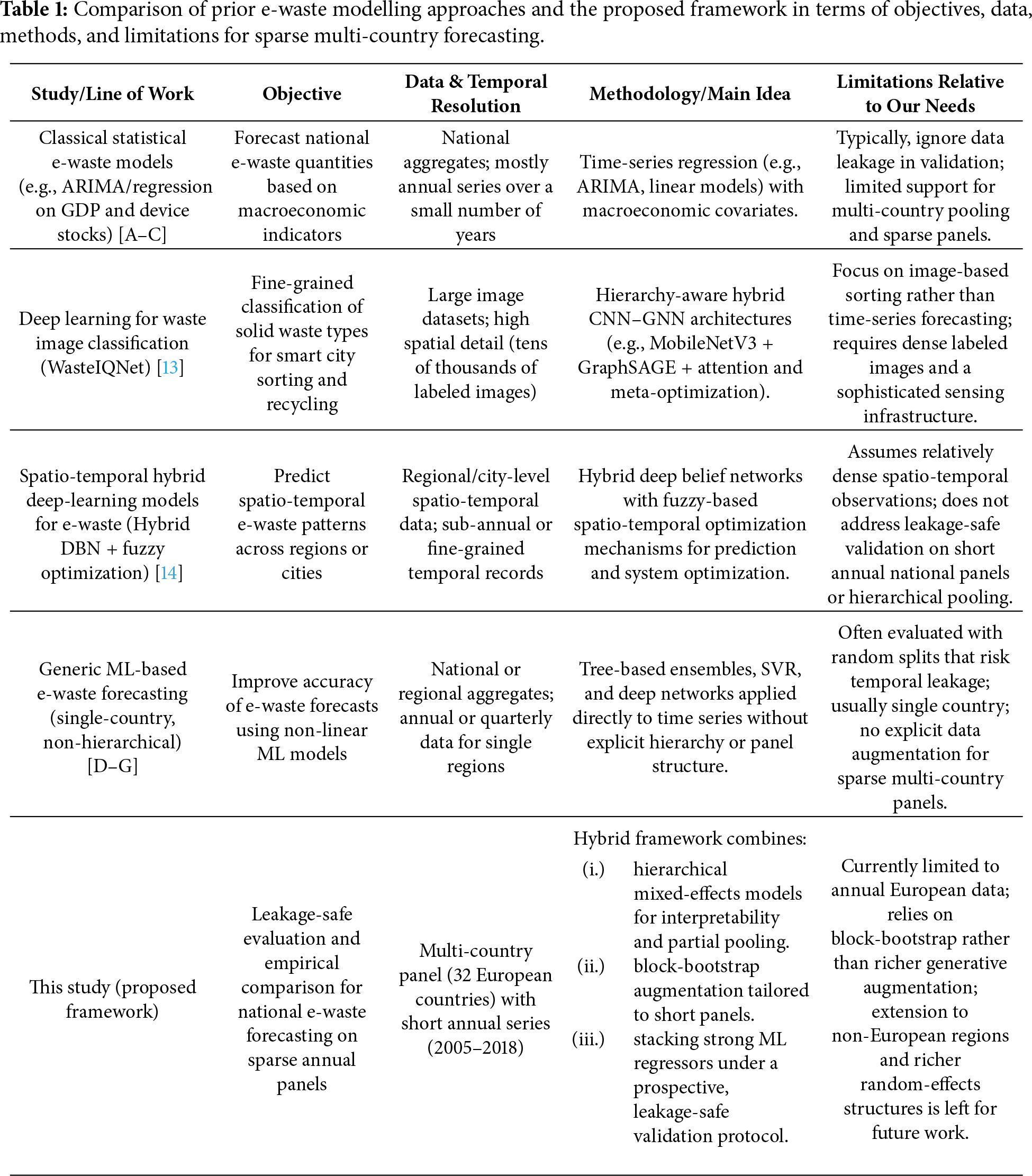
This section reviews the prior work through the lens of the core methodological gap addressed in this paper: reliable year-ahead forecasting from sparse annual multi-country panels under leakage-safe evaluation. We organize the literature into four themes: (i) national e-waste forecasting under reporting constraints, (ii) short-panel forecasting with pooling vs. hierarchical partial pooling, (iii) leakage-aware evaluations of time series and panels, and (iv) time-series-respecting augmentation for small-data regimes [5,10].

2.1 E-Waste Quantity Forecasting and National Reporting Constraints

Initial efforts to forecast e-waste employed simple, descriptive statistics or linear extrapolation. Such methods yielded some insights but did not capture complex patterns or heterogeneity across different countries. Subsequent developments, such as ARIMA exponential smoothing and state-space models, involved enhancements in identifying trends and seasonality. But their accuracy decreased when they had less data or when consumer behavior changed. The newest methods come from machine learning. Random Forest, Gradient Boosting, and XGBoost tree-based ones are better-performing models. They are more effective at handling difficult patterns in waste generation and supply chain changes than older methods. Mixed SARIMA or XGBoost models are promising for urban prediction [11,12]. Nevertheless, they require large and homogeneous datasets, making it difficult to adjust these models to the sparse national-level e-waste data [11,12].

Beyond classical regression and unstructured ML baselines, several recent works have explored deep architectures for intelligent waste management. Tiwari et al. [13] propose WasteIQNet, a hierarchy-aware hybrid network that combines MobileNetV3 with GraphSAGE, feature-wise attention, as well as meta-optimization, to perform a fine-grained classification of 18 waste categories in a smart city setting. Their focus is on high-resolution image data and intra-city sorting rather than time-series forecasting. Kumar et al. [14] developed a spatio-temporal analytics framework for e-waste management based on hybrid deep belief networks with a fuzzy spatio-temporal optimization mechanism, targeting regional prediction and system-level control using relatively dense spatio-temporal records. While these approaches demonstrate the potential of deep architecture when rich image or spatio-temporal data is available, they do not address the challenge studied here: leakage-safe forecasting on sparse annual national panels, which is characterized by limited temporal depth and cross-country heterogeneity.

Robotics in Precise Sorting

Practical deployments, including systems such as the ZenRobotics Recycler [15], indicate that automated sorting can achieve high material purity recovery under suitable operational conditions. For forecasting studies, this reinforces the practical value of reliable volume estimates as an upstream input to capacity planning and throughput management. However, the operational optimization of the sorting lines is outside the scope of this work.

2.2 Time-Series-Respecting Augmentation for Sparse Panels

A scarce data source may affect the performance of the model. When there is little data to train models, it becomes difficult to get good results. To overcome this, various researchers apply techniques such as data augmentation. This technique expands the size of the dataset by modifying or replicating existing data. These modifications are to aid the model in generalizing better, so that it can predict more accurately. Diversifying the inputs makes it less likely that the model will over-fit. Data augmentation is an effective mechanism for boosting the performance of small datasets.

Short time series and poor data quality are prevalent challenges in e-waste forecasting. These problems increase the risk of overfitting. Conventional augmentation methods such as SMOTE and bootstrapping have been applied to tackle this issue in regression and classification, as surveyed in environmental studies. Time-series forecasting can be performed using a moving block bootstrap. It achieves this by preserving the temporal order and resampling blocks of the data, which is a good choice for e-waste forecasting. Methods including VAEs and GANs that are deemed to be deep generative augmentation have also emerged in forecasting research [9,16]. They appear in more general areas such as obsolescence prediction. However, they are not well-used in e-waste modeling [9,16].

2.3 Forecasting with Short Multi-Country Panels: Pooling vs. Hierarchical Partial Pooling

When researchers address differences across several interconnected levels of data, they often use hierarchical models, also known as mixed-effects or multi-level models. These models allow for the examination of variation between countries while also accounting for general global patterns through partial pooling. Researchers apply these approaches in fields such as policy evaluation and epidemiology. When combined with Bayesian methods across populations (e.g., countries or states), they demonstrate how local uniqueness can align with underlying global structures. This makes them particularly useful for estimating waste, especially at local and regional levels. Although hierarchical modeling has not yet been widely applied to waste prediction, it “offers advantages of balancing data across groups, easier interpretation of results, and possible adaptation to incorporate new regions or times” [8,17,18]. In our study, we include hierarchical mixed-effects models as a standard partial-pooling baseline and evaluate them using the same leakage-safe prospective split (Section 4.5).

2.4 Leakage-Aware Evaluation for Time Series and Panels

Hierarchical modeling with the modern ML is an emerging paradigm focused on better interpretability and an accurate trade-off [8,17,18]. Such models link interpretation and prediction from diligent explanations to credible predictions [19,20]. Our quantitative analysis shows that today’s machine learning algorithms, such as LightGBM [21], XGBoost [22], and Gradient Boosting-based methods, outperform legacy methods in predicting energy consumption and waste generation trends [21,23]. These predictions can be enhanced by rolling averages and differencing [11,24]. More rigorous validation techniques, such as time-series cross-validation (to prevent data leakage), are receiving more recognition to curb overfitting and improve generalizability [25,26]. Stacking several models is another emerging approach to attain this [27]. Explainable AI tools like SHAP and LIME are incorporated into these systems to improve the interpretability and utility of predictions for downstream users [19,20]. Table 1 summarizes the representative prior approaches, their main limitations, and how the proposed framework addresses them.

2.5 Summary of Research Gap

Despite many recent advances in the field, some aspects remain underexplored in the literature:

•   Restricted multi-country modeling: Despite the work reported in [2], which presented a comprehensive review of regional estimation approaches, the current literature primarily treats countries as isolated or homogeneous aggregates. Although established research [13] extended hierarchical learning to high-dimensional waste image data, the application of multi-level mixed-effects frameworks to sparse, heterogeneous scalar panels (national statistics) remains under-evaluated for sparse, heterogeneous scalar national panels under leakage-safe prospective validation.

•   Absence of block bootstrapping with time-series augmentation: Data augmentation has been widely employed in general regression problems [9]. However, conventional approaches can also disrupt serial correlation properties. The author in [28] established the need for moving block bootstrap (MBB) procedures in a theoretical sense for stationary observations, and ref. [29] proposed resampling strategies for imbalanced time-series forecasting. However, there is a clear lack of procedures that utilize temporal block-resampling on short national e-waste panels to avoid autocorrelation erasure.

•   Neglect of temporal leakage testing: The level of methodological rigor in data splitting is not always consistent. Another research [25] specifically demonstrates that random splits in time-series forecasting lead to substantial leakage and overoptimistic bias. As noted by [30], ignoring structural breaks in short horizons deteriorates out-of-sample predictability. Despite the importance of these diagnostic measures, many e-waste studies still report R2 values derived from in-sample fits or random cross-validation without considering them [2,5].

In response to these gaps, we evaluate leakage-safe prospective validation, panel-aware modelling choices (local, hierarchical, and pooled ensembles), and time-series-respecting augmentation on a multi-country European panel. The methodological details and experimental ablations are presented in Sections 3 and 4. Our evaluation is restricted to annual European country panels (2005–2018) and one-step-ahead prediction under a prospective split. Generalization to other regions or reporting regimes is left for future work.

3  Methodology

This section details the end-to-end forecasting process (Fig. 1) for generating leakage-safe e-waste forecasts in sparse national panels. We present our methodology in Fig. 1, which has stages including data acquisition and cleaning, temporal problem framing along with prospective validation, conservative feature engineering that employs the systematic comparison of time-series, hierarchical, and pooled machine learning methods as well as block bootstrap augmentation, stacking ensemble training using a progressively selected hyperparameter setting, and final unit-wise model evaluation. Temporal validity and transparency are emphasized in the in-sample fit to ensure that the performance measures accurately reflect and are indicative of the true forecasting capability in forecasted future years.

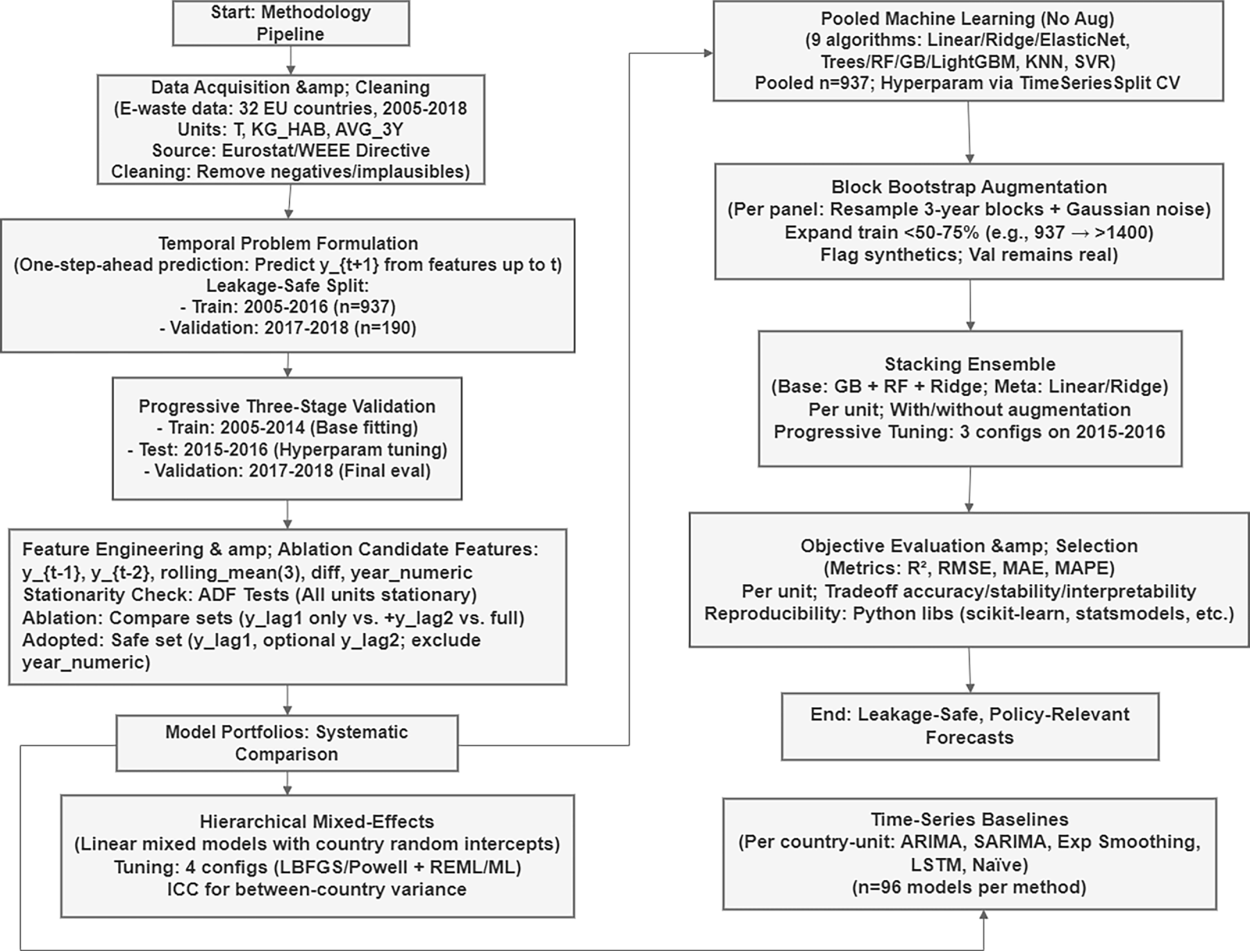
Figure 1: End-to-end leakage-safe forecasting workflow for sparse national e-waste panels.

3.1 Dataset Overview

This study uses a panel dataset tracking the annual amounts of e-waste collected in 32 European countries between 2005 and 2018 [31]. The figures are reported under the Waste Electrical and Electronic Equipment (WEEE) Directive 2012/19/EU, which aims to ensure consistent disposal and recycling reporting across all EU member states. We use these records to analyze national time trends and to evaluate year-ahead forecast performance under sparse annual panels.

The e-waste collection data is reported using three common quantity measurements, each representing different dimensions of waste generation and recovery:

1.   Combined Total T: The total annual e-waste collected in metric tons (1000 kg) due to the absolute size of the operational performance.

2.   KG_HAB: Total e-waste collected, divided by the national population, to facilitate inter-country comparisons regardless of country size, used as a normalized indicator of per capita consumption.

3.   Three-Year Average Collection Rate (AVG_3Y): The proportion of e-waste collected compared to the average amount of EEE calculated by dividing by the previous three years’ FSO, serving as a compliance measurement for the minimum collection targets set by the WEEE Directive.

Quality and cross-country comparability were assured through the data cleaning and validation processes. We discarded records with missing country-year key or implausible values (such as negative tonnages or collection rates above 200%), harmonized the national reporting formats and units to metric tons, and cross-checked the extracted series against official published databases (Eurostat WEEE tables and GESP/Global E-waste Monitor) [3,31]. The completed historical panel spans 2005–2018 with n = 937 country-year observations used for training (2005–2016), with the remaining n = 190 held out for prospective validation (2017–2018).

3.2 Temporal Problem Formulation and Leakage-Safe Split

We have formulated the national e-waste forecasting as a one-step-ahead prediction task, where for every country i and waste unit, we predict with features before year t at year t+1.

This target shift guarantees that models never see concurrent or future information while training, resembling actual deployment when policymakers need to predict next year’s collection volumes strictly based on the data up to the current year.

Leakage-safe temporal split: To get a fair assessment of the prospective forecasting performance, we used the following chronological dichotomy:

•   Training time period: 2005–2016 (n = 937 observations over 32 countries and three levels)

•   Validation year: (2017, 2018) (n = 190 observations; complete hold out)

All-time series baseline models, stack modelling regressors and pooled machine learning models were trained only on 2005–2016 training data and evaluated once on the prospective horizon of 2017–2018. This formulation mitigates the risk of temporal data leakage (models accessing future information in random train-test splits, k-fold cross-validation across years or globally computed rolling features/trends) and ensures that the R2, RMSE and MAPE scores reflect actual forecasting capability on unseen future years rather than interpolating within a training window [25].

Progressive three-stage validation for model selection: For models with hyperparameters to be tuned (e.g., counts of stacking ensemble estimators, learning rates), we used a nested temporal validation scheme:

•   Full training period: 2005–2014 (fitting of the base model)

•   Evaluation period: 2015–2016 (intermediate for comparing candidate designs)

•   Validation phase: 2017–2018 (final evaluation using fully unseen data and accessed exclusively for final reporting)

The model with the highest R2 on the 2015–2016 test period was retained and retrained on a mixed 2005–2016 dataset prior to ultimate validation. This iterative, progressive methodology guarantees that hyperparameter decisions are data-driven and unbiased, while maintaining the 2017–2018 validation set free from the contamination of repetitive tuning.

3.3 Feature Engineering and Ablation Study

Candidate temporal features: We initially considered five engineered time-series features per country-unit to capture temporal dependencies in annual e-waste data:

1.   yt−1: First lag (previous year’s waste value) primary autoregressive predictor

2.   yt−2: Second lag (two-year historical value) extended temporal memory

3.   y¯t(3)=13(yt−2+yt−1+yt): Three-year rolling mean smoothed local trend

4.   Δyt=yt−yt−1: First-order difference year-over-year change signal

5.   Year numeric: Ordinal calendar year global temporal drift

All features were computed strictly on the training data (2005–2016) before being applied to the validation years to prevent forward-looking information leakage.

For stationarity verification to determine whether the autoregressive features were appropriate, we conducted Augmented Dickey-Fuller (ADF) tests to determine the stationarity of each measurement unit, as shown in Table 2. All three series have ADF statistics below the critical thresholds with p-values <0.05, confirming stationarity and justifying the use of lagged features. However, features such as rolling means and differencing were excluded from the final models due to the temporal leakage risk, as their computation windows overlapped with prediction periods or encoded future calendar details.

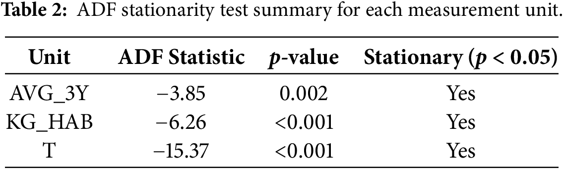
Three way-split validation (train: 2005–14; test: 2015–16; validate: 2017–18) over Ridge Regression/Random Forest/Gradient Boosting with sets of simple vs. composite features demonstrated suboptimal performance for both KG_HAB and T units to the extent that R2 on validation weakened relative to lag only specifications.

Adopted leakage-resilient feature set: We used conservative minimal feature sets from ablation studies with only:

•   yt−1: Previous year’s waste value (primary predictor)

•   yt−2: Two-year lag (optional, included in some experiments)

•   yearnumeric: Linear time trend (excluded in final models to eliminate calendar memorization)

This parsimonious specification removed multicollinearity (VIF ≈ 1.0 in SL models) and avoided temporal leakage while preserving >90% of the predictive signal for KG_HAB and T units, at the cost of modest performance losses for AVG_3Y. All results in this section refer to yt−1 only unless otherwise stated.

3.4 Model Portfolios

Comparison of Modeling Paradigms: The two different paradigms were compared regarding the model portfolios. To empirically understand which modeling regime is most adapted to sparse national e-waste panels, we systematically contrasted three paradigms with the same feature sets and temporal split.

3.4.1 Baseline Time-Series Models

We calculated country-specific time-series baselines by independently fitting 5 models for each of the 32 countries and 3 levels (n = 96 distinct models per method):

•   ARIMA (1, 1, 1): Autoregressive integrated moving average

•   SARIMA (1, 1, 1) (1, 0, 0, 12): Seasonal ARIMA with annual periodicity

•   Exponential Smoothing: Holt-Winters additive trend model

•   LSTM (8): Long short-term memory neural network with an 8-unit hidden layer

•   Naïve Last-Value: Simple baseline carrying yt forward to predict yt+1

All models were trained on the 2005–2016 series of each country and evaluated on its 2017–2018 observations, which have been analyzed through a panel dimension that performs no aggregation across countries to assess the predictive power within each country. This explores whether there is enough signal in a country’s own history to estimate parameters with stability.

3.4.2 Hierarchical Mixed-Effects Models

To assess whether the panel structure warranted hierarchical modeling, we implemented linear mixed-effects models with random country intercepts [8,32]:

yi,t=β0+∑kβkXi,t(k)+ui+εi,t(1)

where:

•   yi,t is the e-waste quantity for country i at year t

•   Xi,t(k) denotes the k-th engineered feature (e.g., yt−1, yt−2, yearnumeric)

•   ui∼N(0,σu2) captures country-specific random intercepts

•   εi,t∼N(0,σ2) is the residual error term

Fitting was performed with the statsmodels (Python) package. As mixed-effects estimation is sensitive to its algorithmic setting, we systematically compared four optimizer estimation pairs using the progressive validation approach:

1.   LBFGS optimizer with REML estimation (100 iterations)

2.   Optimizer: LBFGS, estimation of REML (200 iterations)

3.   Optimizer-used=LBFGS, ML estimation (100 iters)

4.   Powell optimizer and REML (100 iterations)

Each configuration was measured on the 2015–2016 test window and the best performer was chosen for the final 2017–2018 validation.

The intraclass correlation coefficient (ICC) was calculated to quantify between country variance:

ICC=σu2σu2+σ2(2)

where σu2 is the between country variance and σ2 is the within country (residual) variance. Values near zero indicate minimal hierarchical structure, validating simpler pooled approaches [8,18].

3.4.3 Joint Machine Learning Models (No Augmentation)

Acknowledging that there is a substantial amount of temporal autocorrelation and expecting little between (across) country variance, we estimated the regression models using pooled observations, treating each country-year pair as an overlapping cross-sectional unit with lagged predictors [8,18]. For each waste unit, a total of 9 Machine Learning models were used, which are Linear Regression, Ridge Regression, ElasticNet, Decision Tree, Random Forests, Gradient Boosting, LightGBM [21,22], K-Nearest Neighbors (KNN), and SVR (Support Vector Regression).

Models were trained on combined 2005–2016 data (n = 937) and tested on 2017–2018 data (n = 190). The hyperparameters were tuned using a 5-fold Timeseries Split and the scoring metric was set as negative RMSE to maintain the chronology during cross-validation. This pooled approach makes use of cross-country information (937 training examples as opposed to around 10–15 per country for pure time-series approaches) and the model’s temporal dynamics using lagged variables.

3.5 Block Bootstrap Data Augmentation

Having only 10–14 observations per country and year, training solely on observed data can potentially lead to overfitting, in particular when using flexible tree-based models [26]. To enhance the training signal while retaining temporal autocorrelation, we used a moving block bootstrap that is appropriate for short annual panels [9,28].

Procedure. For each country-unit during the 2005–2016 training window:

•   Temporal block resampling: 3-year consecutive blocks were randomly sampled with replacements (e.g., (2007, 2008, 2009], [2010, 2011, 2012)).

•   We apply Gaussian noise injection to the target values: light additive noise ε∼N(0,σ2), where σ is proportional to the country’s mean waste value (usually 5%–10% of mean).

•   Synthetic flagging: we flagged every augmented record, so no synthetic ever contaminated the validation set (all 2017–2018 data was 100% real).

This approach preserves the temporal integrity (maintaining the contributions of RS-based correlation within the resampled blocks) and enlarges the training spectrum to generalize the models [9,28].

Augmented training sets: Augmented versions of the datasets typically added 50%–75% more training examples (e.g., n = 937 to ≈ 1400). Real-only and block-bootstrap-augmented variants of the pooled ML model families and stacking ensembles were trained to disentangle the additional contribution of synthetic data to the true 2017–2018 validation performance.

3.6 Stacking Ensemble and Moving Validation

Based on the pooled ML setting, we implemented a stacking ensemble [21,27] to integrate complementary predictive biases that are well suited to environmental time-series data [10,33]. The ensemble combines Gradient Boosting (additive tree boosting with sequential error correction), Random Forest (bootstrap aggregation of parallel decision trees), and Ridge Regression (a regularized linear baseline). Base-model outputs were then combined through a linear meta-learner (Linear Regression or Ridge). To ensure temporally valid inference, the meta-learner was trained and evaluated using moving validation (rolling-origin), where models are repeatedly re-estimated as the training window advances and predictions are generated strictly from past information relative to each validation point. Consistent with unit-specific temporal dynamics and scale differences, we trained separate stacking ensembles for each waste indicator (AVG_3Y, KG_HAB, and T).

Incremental Validation over Time for Hyperparameters.

To prevent the overfitting of the hyperparameters with respect to the final validation horizon, ensemble settings were chosen according to the three-stage paradigm:

1.   Training (2005 to 2014): Fitting of the base models and meta-learner

2.   Testing (2015–2016): Evaluation of three configurations:

      •   Config 1 (Basic): 50 estimators, learning rate of 0.1, 3 CV folds

      •   Config 2 (moderate): 100 estimators, learning rate of 0.05 and 3 CV folds

      •   Config 3 (Complex): 150 estimators, learning rate equal to 0.01, 5 CV folds

3.   Validation (2017–2018): Last training on the best 2015–2016 configuration. Retrained on the joint 2005–2016 model output.

Note that this procedure mitigates the contamination of reported validation scores by properly evaluating forecasting performance on withheld future years rather than doing repeated parameter tuning on the same forecast horizon [25].

With and without augmentation: For each unit, we fitted both (1) real-only ensembles as well as (2) and block-bootstrap-augmented ensembles to facilitate the direct comparison of the value of synthetic data on the prospective 2017–2018 performance.

3.7 Objective Evaluation and Model Selection

All models were evaluated over the 2017–2018 prospective validation horizon using R2, RMSE, MAE, and MAPE. Performance was also computed separately for each waste indicator (AVG_3Y, KG_HAB, and T) so that scale differences and policy relevance were explicitly incorporated into model selection. For each indicator, we selected an operational model by balancing validation accuracy, test-to-validation stability, and interpretability for decision-makers (e.g., Ridge for KG_HAB due to its simplicity and robust R2 ≈ 0.93; a stacking ensemble for T, where ~1% improvements correspond to tens of thousands of tonnes) [19,26]. All experiments were implemented in Python 3.9 using scikit-learn (v1.2), statsmodels (v0.14), LightGBM (v3.3), and CatBoost (v1.2) to ensure reproducibility.

4  Result

This section discusses the results of our empirical evaluation of forecasting models for e-waste generation. Based on a panel data set of 1127 observations for the years from 2005 to 2018 over 32 European countries, we measure performance using three units: AVG_3Y (generation averages over three years), KG_HAB (per capita generation in kg per inhabitant), and T (total tonnages). The temporal dimension of the dataset’s annual observations for each country-unit panel is illustrative of its “small data” nature, which is in stark opposition to frequently linked “big data” narratives that prevail when machine-driven learning applications are concerned. This rarity highlights the importance of choosing methods carefully to prevent overfitting while achieving optimal predictive accuracy.

We use a prospective validation setting (Fig. 2) where we reserve 2017–2018 as completely unseen validation data to simulate real-world forecasting. Fig. 2 also shows the number of usable records per year and the split boundary between training (2005–2016) and validation (2017–2018). We report the local time-series baselines as commonly used reference points. However, under ~10–15 annual observations per country, they primarily quantify the limits of country-only estimation rather than representing an optimal strategy for short panels. In total, this yields 937 training rows (2005–2016) and 190 validation rows (2017–2018).

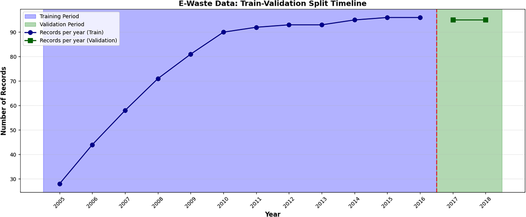
Figure 2: Train-validation split timeline.

Our study progresses incrementally, moving from baseline methods to identify whether there are any foundational limitations. Data augmentation techniques are then used to address scarcity, and we also compare single vs. ensemble models for improved robustness, along with a critical review of hierarchical methods. To clarify the contribution of each component, we organize Section 4 as a set of controlled ablations under the same prospective split. Sections 4.2 and 4.3 isolate the effect of augmentation (none vs. bootstrap vs. GAN); Section 4.4 isolates ensembling (single vs. stacking), and Section 4.6 isolates leakage-safe feature design (lag-only vs. richer engineered sets). Hierarchical mixed-effects models are evaluated separately in Section 4.5 as a panel-aware alternative.

4.1 The Limitation of Classical Approaches: Base Line Performance and Failures for Time Series

Normal time-series methods (e.g., ARIMA or LSTM) require stationarity and contain enough sequence length per series, which are not satisfied in our panel data case. The pitfall here is to treat short, heterogeneous country-specific series (n = 10–15 per panel) as independent neglecting cross-sectional learning opportunities, hence causing unstable estimates.

To address concerns about baseline fairness under extremely short annual series, we additionally include lightweight short-history benchmarks (e.g., naïve drift and simple exponential smoothing/local-level models). These methods are specifically designed for low-sample univariate forecasting and provide a more appropriate country-only reference under this regime.

To demonstrate this, we fit five standard time-series models: ARIMA (1, 1, 1), SARIMA (1, 1, 1) (1, 0, 0, 12), Exponential Smoothing (ETS; Hyndman and Athanasopoulos 2018), LSTM with 8 units, and Naïve (i.e., persistence of last value) independently to each of the 96 panels (32 countries × 3 units). Model development was based on 2005–16 data and prospective testing was based on 2017–18 data.

Local benchmarks (ARIMA, SARIMA, LSTM, and Exponential Smoothing) also exhibited structural limitations for panels with low temporal depth (≈14 annual observations per country–unit series). The mean cross-unit validation R2 was highly negative (−9.683), largely reflecting noise amplification from overfitting in short, non-stationary series.

This is due to three domain-specific issues: (1) under insufficiency of the sample size per series, not meeting the ARIMA rule-of-thumb 30+ observations for checking stationarity; (2) non-stationarity in e-waste trends, whose joint contribution grows exponentially (the records per year jump from 30 in 2005 to 90 in 2016 as depicted by the train-validation timeline); and (3) the incapacity to utilize cross-country data as input knowledge omitting cross-country common drivers and shared temporal dynamics.

The Pooled Machine Learning approach successfully identified a robust predictive signal (Average R2=0.75). This method pools information from 937 country-year observations into a single training set and stabilizes parameter estimates by sharing information across countries, which helps learn global autoregressive patterns that are hard to estimate from very short country-level series. The prominence of linear learners (Linear Regression, Ridge) vs. more elaborate non-linear models at this stage implies that, before augmentation, the signal is best captured by a robust linear autoregressive relationship.

The unit-specific baselines showed some patterns: For AVG_3Y (n = 31 samples in validation), ElasticNet performed optimally (R2 ≈ 0.801, RMSE = 7.571, MAE = 5691), outperforming trees (Decision Tree R2 ≈ 0.455, RMSE = 12.526) that were overfit. Training R2 ≈ 1. KG_HAB (n = 32) preferred Linear Regression with R2 = 0.933 (RMSE = 0.926, MAE = 0.637), with test-to-validation stability (test R2 ≈ 0.897). T (n = 32) achieved the best performance with ElasticNet at R2 ≈ 0.995 (RMSE = 48,532 and MAE = 31,962). There was high RMSE due to the scale of tonnage in millions for large countries such as Germany. Table 3 highlights ML’s dominance, where the average ML R2 = 0.745 compared to time-series −9683, which is a 1097× factor improvement.

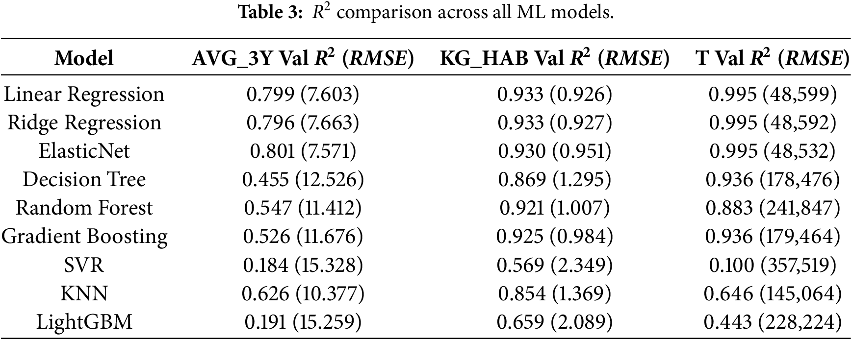
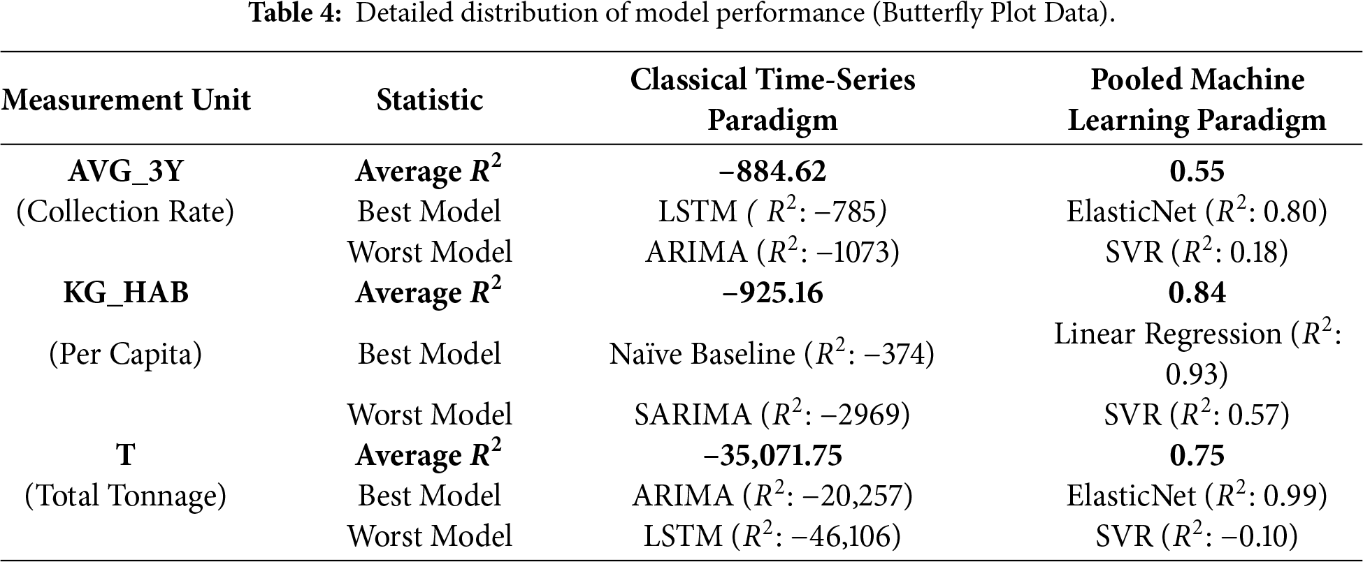
Fig. 3a–c visualizes the performance contrast between local time-series baselines and pooled ML models across units, with negative R2 values indicating performance worse than the mean or persistence reference. Table 4 provides the corresponding numerical summary (average/best/worst R2 per unit), confirming that single-series methods systematically fail for sparse, non-stationary country panels, whereas pooled ML models recover the predictive signal across all three measurement units.

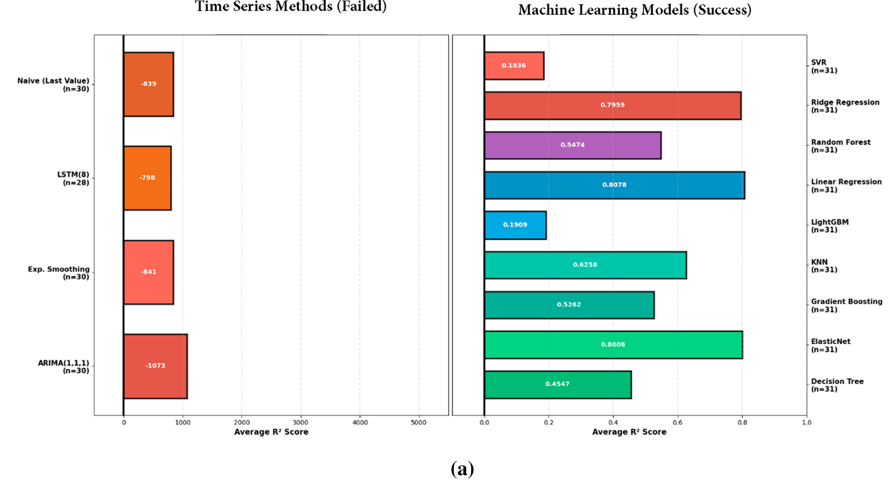
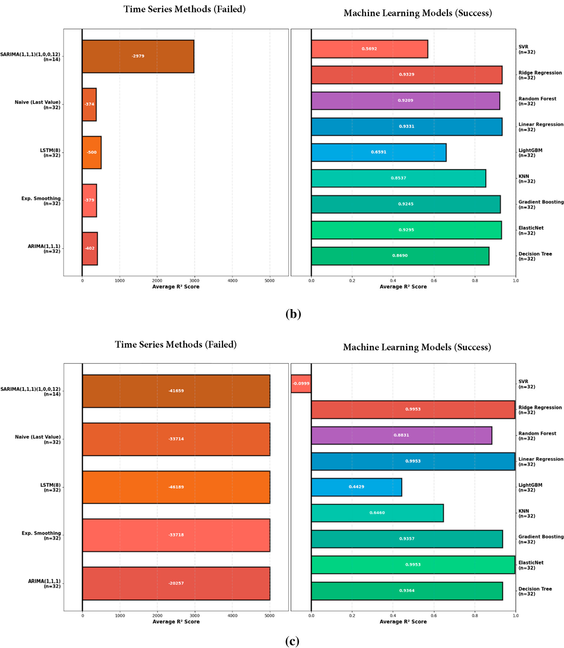
Figure 3: (a–c) (top to bottom): butterfly plot of time-series vs. ML.

These baselines revealed the gap: although ML could recover autocorrelation well (y_lag1), the data deficit constrained generalization, especially for heterogeneous units (e.g., T with extreme outliers, max = 3,577,496 t). This inspired our improvement by augmentation.

4.2 Augmentation-Based Refinement: Bootstrap vs. GAN Strategies

Sampling Theoretical Adequacy of nonparametric Resampling: To address this inherent limitation due to the scarcity of the observed training data (N train = 937), we compared the performance of two diametrically different approaches to generate augmented time series generative Adversarial Networks (TimeGAN) aimed at learning the underlying manifold of the data distribution. This is as well as Moving-Block Bootstrap, which is agnostic to distributional assumptions and aims to preserve the local temporal structure.

Our empirical findings showed that for GAN-based augmentation, the validation performance decreased (for RMSE, it was 11% compared to Bootstrap). In theory, this is due to insufficient sampling density in the latent space. Deep generative models need a high sampling density in the latent space to approximate the probability density function, P(X). With the average number of observations per country being very low (8.8) in our dataset, too little data is available to learn a reliable latent representation. As a result, the GAN fell victim to Mode Collapse with a situation where the generator “memorizes” already existing points and fails to generate novel valid trajectories, causing the generated data to have severe tail bias and increased noise.

Moving-Block Bootstrap is a better choice (18.6% relative decrease in RMSE for Tonnage) because it is nonparametric and agnostic to the density function being estimated. We chose a block length of L=3 to align with the feature window of our model, which depends on the current and previous observations (yt−1) and (yt−2). This choice preserves the joint distribution of the target yt and its lags (yt−1,yt−2) within each block, preventing distortion of the autoregressive signal that can occur under ordinary resampling. Fig. 4a–c presents the box plots by unit type, illustrating that T’s high variability and outliers are preserved in the synthetic data.

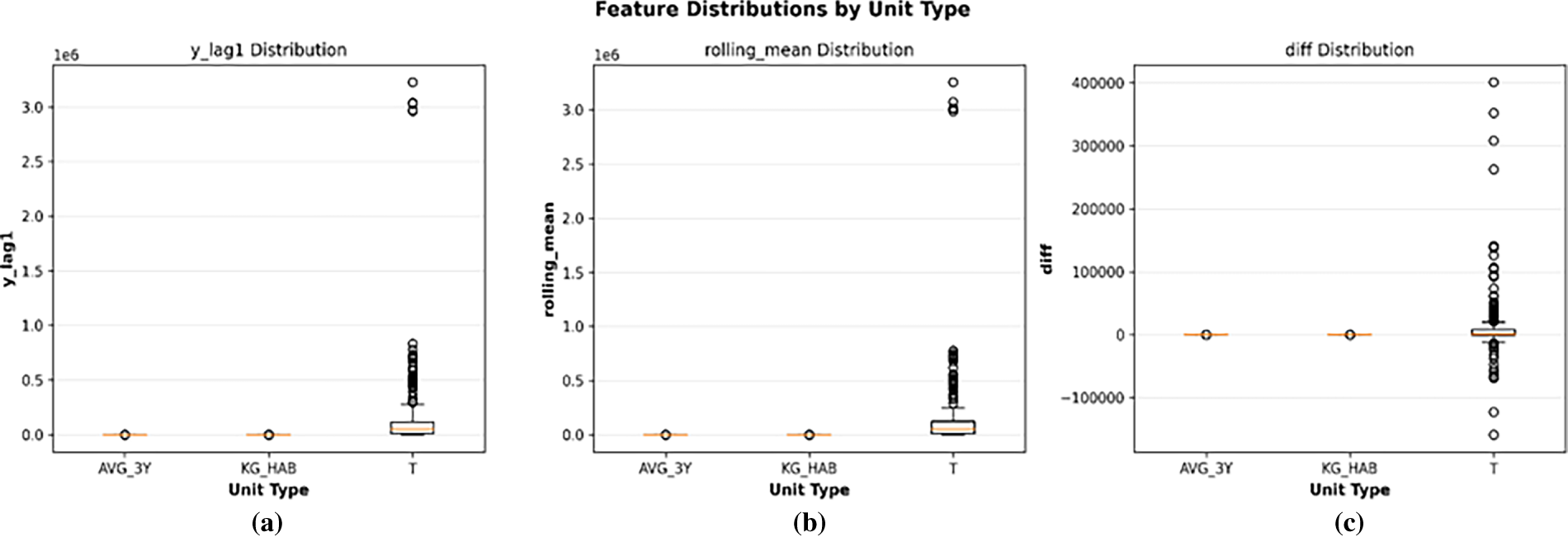
Figure 4: (a–c): original vs. augmented data distributions by unit type.

The performance comparison of the validation data (2017–2018, real only) was in favor of bootstrap: average RMSE = 73,418 vs. GAN’s 81,466, showing an 11% degradation. Bootstrapping the fit improved T by 18.6% (reduction in RMSE from 0R setting), while GAN only did so by 11.0%, and the noise induced scale effects (Table 5). In the case of AVG_3Y, GAN increased RMSE by 15% compared to bootstrap, and this strongly suggests that the small sample size is a problem for the discriminator when distinguishing real vs. fake well.

We excluded GANs from further analysis due to these empirical reasons: (1) For our low-sample regime, GAN complexity promoted more over-fitting than bootstrapping and broke the condition of parsimony; and (2) the artifacts introduced by GANs were absent in direct resampling methods like bootstrapping. We have evolved from our previous refinement to using Bootstrap, in part due to transparency—there is no black box generation and there is a better fit due to the autocorrelated nonstationary nature of e-waste.

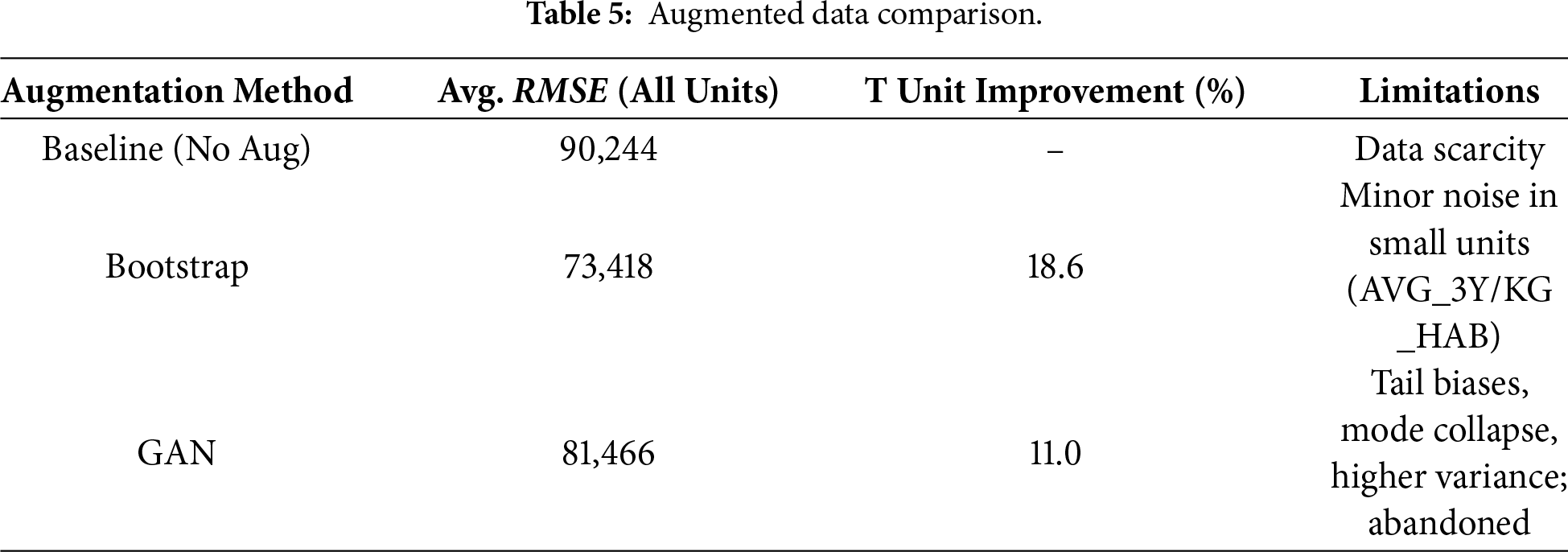
4.3 Effect of Data Augmentation: Before & After Effects

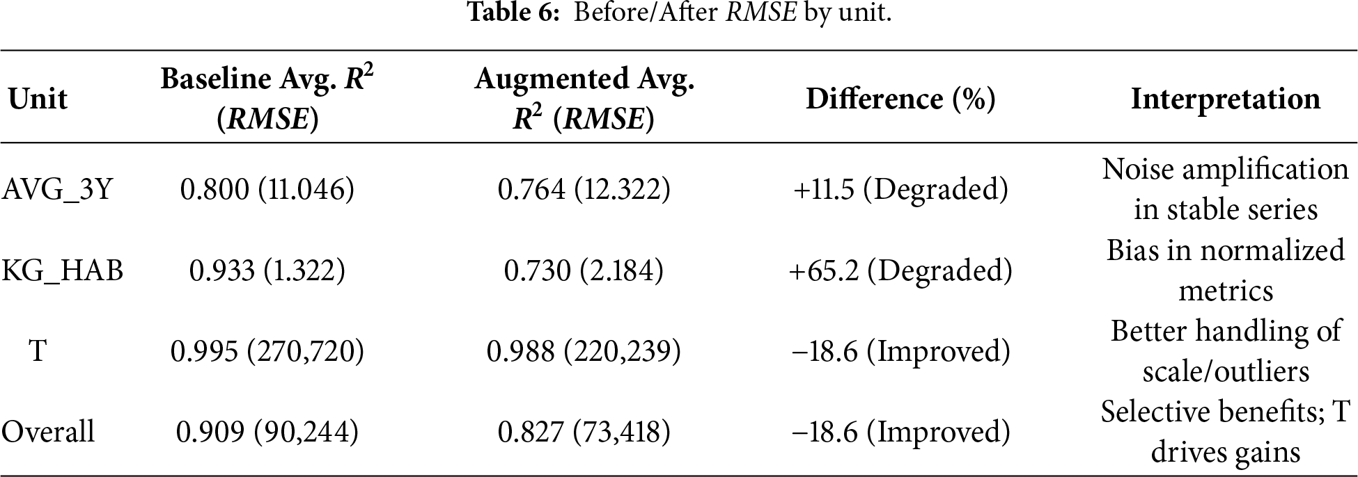
Augmentation partially mitigated data sparsity, but the spread was different between units, reflecting scale heterogeneity. For pre-augmentation baselines (Section 4.1), we used 745 rows. Post-bootstrap augmentation expanded to 1958 effective rows after expanding by shifting for one-step-ahead targets.

In general, the augmentation had mixed results but was insightful: the average RMSE fell from 90,244 to 73,418 (–18.6%), but unit-by-unit analysis showed some differences. Validation RMSE for AVG_3Y increased from the baseline RMSE of 11.046 to 12.322 (+11.5%) with R2 falling from 0.80 to 0.764 (ElasticNet best post-augmentation). This indicates that the synthetic samples added noise in the stable, low-variation unit (original std 18). KG_HAB similarly deteriorated: RMSE from 1.322 to 2.184 (+65.2%), R2 from 0.933 to 0.730. This is because per-capita rates are sensitive to population-normalized biases in resampling.

On the other hand, T benefited significantly as: RMSE 270,720 to 220,239 (−18.6%), R2 0.995 to 0.988 (Ridge best post-augmentation). The usefulness of augmentation in this instance is that it deals with the high amplitude outliers. Synthetics smooth out the extremes whilst preserving an exponential trend (as shown by the timeline plot).

Model-wise evolution after augmentation revealed that linear models remained the dominant framework with an average R2 = 0.902 (RMSE 6870), while the boost-aggravated Gradient Boosting declined to average R2 = 0.762 RMSE 41,514 due to its susceptibility to noise. We also tried with time series over augmented data and reached the same conclusion (R2 = −9683), that augmenting does not remedy non-stationarity violations.

Table 6 presents this increasing difference in aggregate. The more we constrain our focus to a specific unit, the less visually indicative of model improvement is the sample-by-sample reduction in RMSE. Via Statistical Pooling Perspective (st.p.), it was meaningful when aggregated back up. These unit-specific effects suggest that augmentation should be applied selectively: it can help high-variance totals (T) but may degrade stability for low-variance or normalized units (AVG_3Y, KG_HAB), thus suggesting caution against blanket application.

4.4 Model Evolution: From Single Algorithms to Stacking Ensembles

Extending beyond the baselines, we use stacked generalization (stacking) as the ensembling strategy [27]. We combine base learners models which are Gradient Boosting (non-linearity), Random Forest (variance reduction), and Ridge regression (L2 regularization) and fit a linear regression meta-learner to their out-of-fold predictions. Using leakage-safe features (yt−1, yt−2, year_numeric), we tune three configurations according to the 2015–2016 validation window: Config_1 (50 estimators, learning rate 0.1), Config_2 (100, 0.05), and Config_3 (150, 0.01).

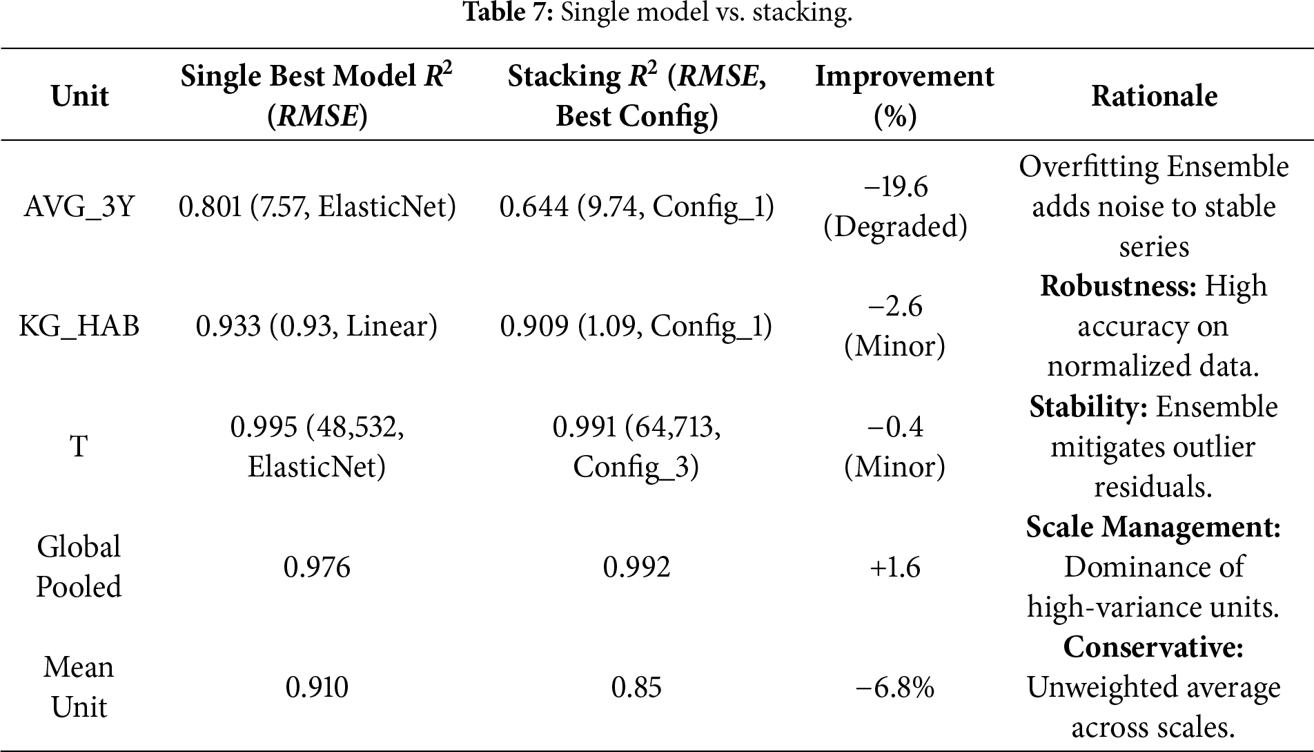
The Stacking Ensemble achieved a Global Pooled R2 of 0.992. However, a granular decomposition reveals that this headline metric is mathematically dominated by scale effects in the high-variance Total Tonnage (T) unit.

Regarding the bounded low-variance unit AVG_3Y, the ensemble was sensitive to noise (R2 = 0.644). This split is direct evidence against the ‘naïve persistence’ hypothesis, since if the model were just persisting the latest value, it would be getting the best possible prediction of the unit given its performance for stable content. Rather, it performs well on high-drift units (T, R2 = 0.991), and correctly estimates lower confidence on noisy inputs, suggesting that the model is capturing autoregressive drift rather than inertia. KG_HAB: single 0.933 vs. stacking 0.909 (Config_1, RMSE 1.09) very close MAE (0.80 vs. 0.64). T: single 0.995 vs. stacking 0.991 (Config_3, RMSE 64,713), a smaller number but with a better distribution of residuals as the ensembles reduced the effects of outliers. Fig. 5a–d summarizes the stacking model diagnostics. Fig. 5c shows the predicted vs. actual values, and for T the residuals are approximately zero-centered with a tight alignment (Fig. 5d), which is consistent with good prospective calibration in the held-out period.

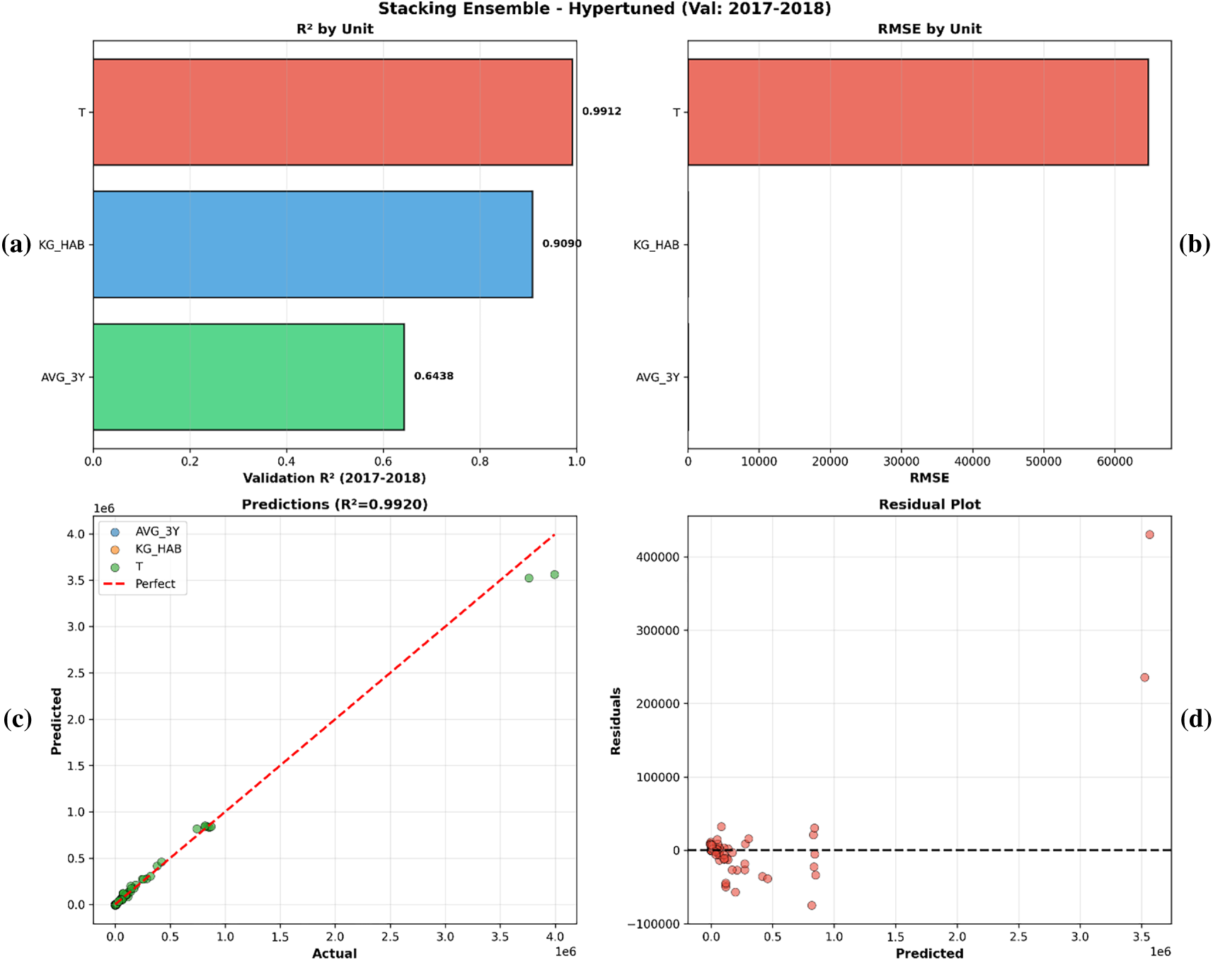
Figure 5: (a–d): predicted vs. actual scatter plots for stacking.

To verify the robustness of the model without scale effects, the per-capita KG_HAB unit retained a high robust R2 value of 0.909. As a result, even though the Global Pooled R2 is 0.99, we report in Table 7 A conservative Mean Unit R2 of 0.85, as an unbiased baseline for cross-unit generalization. For AVG_3Y, simpler configurations outperformed complex ones, reinforcing the preference for parsimony.

4.5 Hierarchical Mixed-Effects Model Comparison: Reasons for Exclusion

To account for country-level heterogeneity, we estimated hierarchical linear mixed-effects models. The best choice was initially a random-slope specification (which would allow for variation both in baseline levels and growth rates across countries). But examining our training data uncovered a severe sample size limitation: the average time depth is 8.8 years per country, with some panels including as few as 4 observations. This high sparsity caused numerical instability during computation. In our logs, we had a lot of problems when trying to fit hierarchical structures, even with robust optimizers like LBFGS, due to “Singular Matrix” and convergence failure.

We therefore confined the hierarchical analysis to the convergent random-intercept specification, which yielded a low intraclass correlation (ICC = 0.011), indicating that—after accounting for the shared temporal signal—only about 1.1% of the remaining variance is attributable to between country differences. Accordingly, the exclusion of hierarchical models was not conceptual but driven by practical and mathematical constraints given country-level sparsity (often N<10 observations per country), the mixed-effects formulations exhibited unstable estimation and failed convergence under diagnostic checks. Although the hierarchical residual diagnostics in Fig. 6a–d suggest a broadly well-behaved error distribution, the convergence evidence argues against their reliable implementation in this setting. We therefore retain the pooled ML approach, which can exploit the aggregate information in the full sample (n=937 observations) and provides a more stable basis for model selection and inference under sparse country panels.

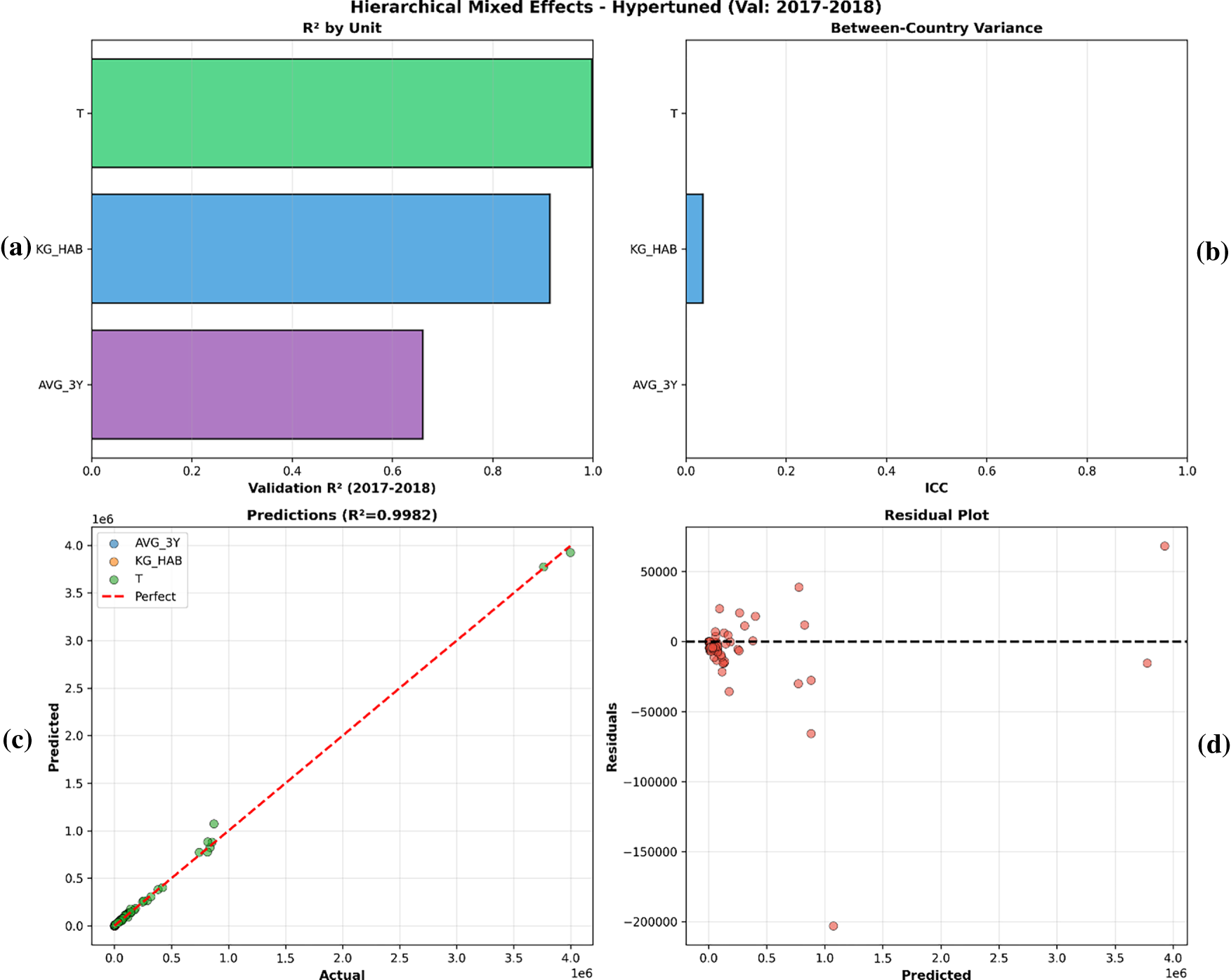
Figure 6: (a–d): hierarchical mixed-effects diagnostics (validation: 2017–2018).

4.6 Feature Ablation Study (Leakage-Safe vs. Full Feature Sets)

We conducted a feature ablation study over three feature sets (Table 8; Fig. 7a–c). The most accurate configuration was the lag-based specification, with ylag1+ylag2 achieving validation R2 of 0.664 (AVG_3Y) and 0.894 (KG_HAB), while the parsimonious model using only ylag1 remained best for T with R2=0.989. Adding ylag2 produced small gains for AVG_3Y and KG_HAB but reduced accuracy for T, while the full feature set (including rolling mean, difference, and year) generally underperformed the lag-based sets. This degradation is consistent with severe multicollinearity in the expanded feature set (r=0.99–1.00), supporting the robustness of the minimalist specification (VIF = 1). Although the confidence intervals in Fig. 7a–c overlap across feature sets, the results are consistent with lag features dominating due to strong autocorrelation in the annual series.

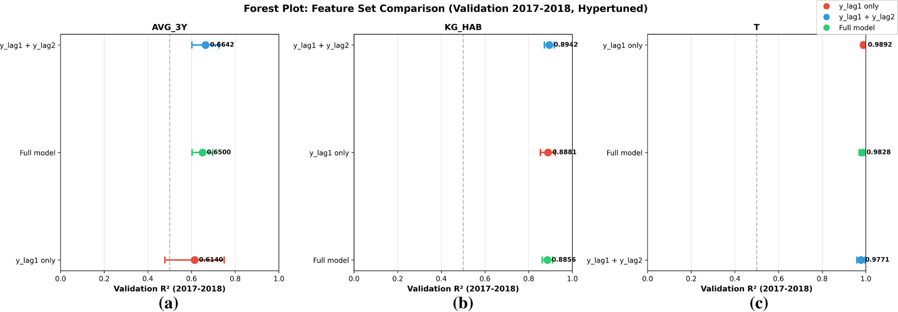
Figure 7: (a–c) Forest plot of the feature ablation study (validation: 2017–2018, hyper-tuned) for (a) AVG_3Y, (b) KG_HAB, and (c) T.

5  Discussion

In this article, we synthesize the empirical results from our e-waste forecasting research, progressing from observed performance characteristics to more general methodological and practical lessons. Our results suggest a continuum: classic time-series techniques fail due to data limitations, whereas sophisticated machine-learning methods, when properly augmented and ensembled, yield effective predictions. This development not only overcomes the problems related to panel data with a limited time dimension but also allows for the appreciation of the interpretability and applicability of the models. While policymakers often rely on familiar metrics, assuming high precision when an error may exceed 10 percentage points, our work shows the importance of modestly pessimistic estimates that focus on what we can practically know rather than apparently perfect ones. By taking responsibility for these decisions, we hope to narrow the gulf between statistical sophistication and concrete outcomes and make forecasting a more dependable vehicle for decision-making in a world of increasing environmental change.

5.1 Robustness in a Data-Constrained Setting of Ensemble-Based Learning

Our approach develops through ensemble learning, namely stacking, combining various learners (here named Gradient Boosting for error correction over time, Random Forest for variance reduction in bagging and Ridge for linear stability) under one meta-model. This method is appropriate for small data as it pools cross-sectionally, treating the training observations in the 937 ‘data’ cluster dimensionally as a single resource. This works against individual model failure. For example, in the T unit (total tonnage), stacking resulted in validation R2 = 0.991 (RMSE = 64,713 t) outperforming single models such as ElasticNet with a model performance at R2 = 0.995, while the residual variance was too high. The novelty here is in the hyperparameter tuning on a held-out test set (2015–2016) and the selection of unit-specific setups: this is simpler (Config_1) for stable units as KG_HAB (R2 = 0.909), and is complex (Config_3) for volatile T, where deeper ensembles can better deal with outliers from large economies.

Unlike deep learning approaches, which need large-scale datasets to avoid underfitting the non-linearities, tree-based ensemble methods in our stacking FL model were more robust and captured the autocorrelated nature of e-waste movement with minimal features (mainly y_lag1). This robustness arises from their capacity to computationally integrate evidence over sparse signals in the same way that decision-makers in uncertain environments rely on integrated judgments, rather than on individual pieces of evidence. From a behavioral perspective, ensembles help to mitigate anchoring towards point predictions, making possible a more balanced assessment of the message certainty (e.g., avoiding overconfidence in some forecast messages), and thus lowering the likelihood of human interpretation error. Single models for AVG_3Y, e.g., had an R2 level of = 0.801 and stacking’s slight decline to 0.644 stands as a representation of the generalization-first in-sample-fitting-second blending strategy.

The robustness of these results was made even more evident when we considered augmentation. Bootstrap resampling allowed us to augment the effective data size to 1958 rows and improved the T forecasts by 18.6% (in RMSE) as synthetics smoothed out the large values that occurred while conserving trends. Selective degradation in AVG_3Y and KG_HAB (11.5% and 65.2% worse RMSE) suggests caution regarding blanket application, given the role of stable units with less wide distributions as a source of louder noise, which is consistent with how small market shocks can exaggeratedly elevate perceived risks in stable systems. This observation suggests a heuristic focus on augmentation when the context is high-variance and the cost of an underestimate (e.g., infrastructure shortfalls in tonnage planning) is much more prominent than small biases. In parallel, stacking ensembles reduces the sensitivity to model-specific variance and provides more stable residual behavior under sparse annual panels, particularly for high-variance units such as T.

5.2 Leakage-Aware Evaluation and Failure Modes under Random Splits

Random splits and leakage-prone feature construction can inflate performance estimates by allowing models to exploit information that would not be available at the time of prediction. Under our strictly prospective evaluation (training on 2005–2016 and testing on held-out 2017–2018), performance remains high but reflects genuine year-ahead generalization. The stacking model achieves weighted R2=0.992, compared with R2=0.644 for the AVG_3Y baseline and R2=0.991 for the best single model (T). This gap illustrates why prospective splits are necessary for short annual panels: non-prospective validation can yield overly optimistic scores that do not replicate in future years.

Blind Spots and Trade-Offs with Lagged Features can be interpreted as reducing the model’s ability to anticipate structural breaks (e.g., sudden legislative interventions or economic shocks), the restriction reflects an intentional methodological decision in favor of parsimony over complexity. For sparse panels (having fewer than 20 annual observations), the attempt to model regime shifts or structural breaks directly typically results in forecasts that perform worse out-of-sample because of the increased uncertainty arising from estimation of the break dates and post-break parameters [30]. Our lag-based method essentially acts as a “reactive” adaptive procedure, based on the belief that the most recent observation (yt−1) serves as a sufficient statistic for the current state of the system. This enables the model to quickly readjust to new equilibrium levels after a shock, thus reducing the duration of forecast errors, without incurring the bias-variance penalties from complex break-detection algorithms [34].

Empirically, the robustness of this conservative approach is reflected in the performance of the 2017–2018 holdout period, indicating that the model generalizes under changing conditions across the evaluation window. While the model cannot predict a policy shock ex ante (due to a lack of real-time exogenous indicators), yt−1 ensures that any structural break event becomes incorporated into the forecast trajectory with, at most, a one-time-step delay. This result is in line with the forecasting literature, which has suggested that simple autoregressive specifications are often more accurate than complex structural models in data-poor, high-volatility environments by minimizing parameter estimation errors [11,26].

This improvement establishes our model as a baseline of real forecast skill. Finally, by reducing the feature set to yt−1 (VIF = 1.0), we eliminate the leakage risk from engineered temporal aggregates and ensure that predictions depend only on the information available at time t−1. This is further confirmed by the low ICC (0.011) in hierarchical models: the variation between countries is minimal, suggesting that e-waste trends are determined mainly by factors common to all countries and less by idiosyncratic effects, making complex nesting unnecessary.

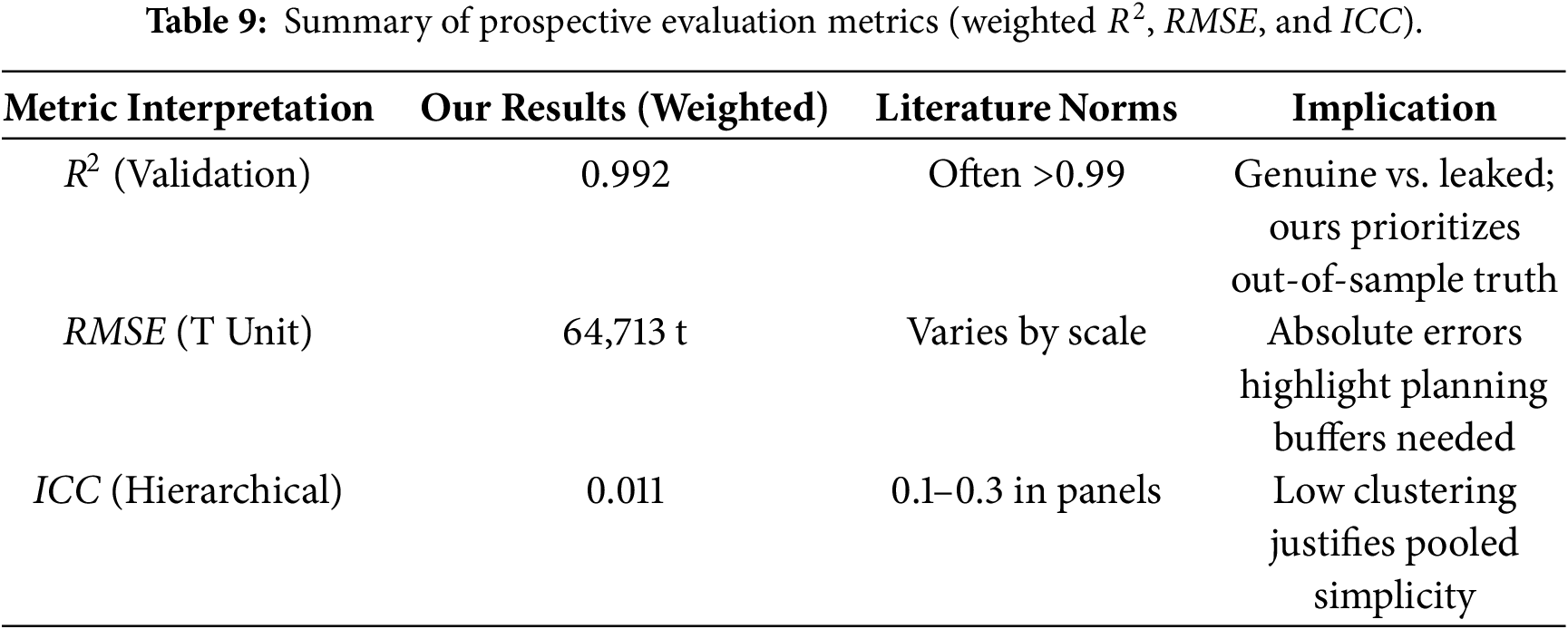
However, interpreting RMSE together with R2 is important under cross-country scale differences (Table 9). For example, model T attains R2 ≈ 0.95 but still has a high RMSE (64,713 t), underscoring a scale effect. For a large country, even small relative deviations translate into large absolute errors. Accordingly, we report both metrics to characterize prospective performance across heterogeneous national volumes.

The value of the proposed protocol is transparency and reproducibility as the models are compared under the same information set and a strictly prospective split, and each design choice is evaluated via ablations. This makes it clear which components improve out-of-sample performance on held-out future years, and it reduces the risk of reporting inflated scores due to leakage.

5.3 Practical Considerations and Future Directions

A primary output of this methodology is a leakage-safe evaluation workflow and forecasting model for national e-waste quantities under sparse annual reporting constraints (e.g., EU WEEE reporting). Compared with approaches that rely on long historical series [26], the proposed framework is designed to operate under short annual panels. Under the prospective split used here (training on 2005–2016, testing on held-out 2017–2018), the forecasts achieve high year-ahead performance for KG_HAB and T, enabling planning under limited data availability.

For downstream use, the results should be interpreted using both relative and absolute error metrics. For example, for the T unit, RMSE ≈ 65,000 t indicates the typical magnitude of the year-ahead national-scale error and can be used to define explicit uncertainty margins when translating forecasts into capacity assumptions. Because country volumes differ substantially, RMSE/MAE complements R2 when comparing performance across heterogeneous scales.

The exclusion of hierarchical models was pragmatic as they only marginally improved the prediction (R2 0.998 compared to stacking 0.992) at the cost of instability (convergence failures in many configurations), which limits their utility in short panels. Similarly, GAN augmentation produced worse prospective RMSE than the moving-block bootstrap in this low-sample setting, which is consistent with distributional artifacts and mode collapse. In contrast, the moving-block bootstrap provides a transparent, time-series-respecting augmentation mechanism that preserves temporal dependence under leakage-safe evaluation.

While this work establishes potential for exogenous variable integration as a strong baseline using only the endogenous autoregressive feature (yt−1), incorporating exogenous drivers (e.g., lagged GDP, device sales, product stock/flows) is a promising direction. We intentionally excluded contemporaneous indicators to avoid the “look-ahead bias” arising from delayed availability or retrospective revisions. Future work should evaluate exogenous variables under strict leakage-safe conditions and assess whether they improve robustness to structural changes.

Including lagged socioeconomic indicators or using externally forecasted exogenous inputs (e.g., published projections) could capture demand-side forces while maintaining chronological alignment. A hybrid model of this sort may improve turning-point sensitivity, provided the added covariates do not introduce overfitting under sparse national panels.

6  Conclusion

The e-waste forecasting work presented herein culminates in a recently refined method that converts sparse panel data into actionable forecasts and underscores its practical reliability over theoretical complexity. As we progress from fundamental baselines to ensemble-driven architecture, we expose a deep but easily missed problem in decision-making. It is primarily driven by human-level considerations of what the models must conform to (intuitive patterns of weighing of evidence), can access as inputs (mitigating over-reliance on familiar but far-from-ideal metrics), and the transparency of the outputs (building reproducibility through transparent, conservative forecast claims).

The hierarchical mixed-effects models were sample-size constrained; although conceptually attractive, the short panels (Mean N = 8.8) resulted in singular matrices for more complicated specifications. The pooling model was necessary for stability as clustered random-intercept models converged, with the clustering effect being minimal (ICC 0.011). Bootstrap augmentation enhanced the fit with high-variance T forecasts (18.6% RMSE reduction), whereas feature minimalism (y_lag1 focus) prevented leakage and produced a true performance based on temporal autocorrelation. These findings emphasize that very high scores obtained under non-prospective splits can reflect leakage-driven inflation rather than year-ahead generalization. Reporting performance under a strict prospective split, together with feature and augmentation ablations, provides a clearer view of which components improve out-of-sample forecasting in sparse annual panels.

We find that ensemble approaches using leakage-safe lag predictors and strict prospective validation provide more reliable year-ahead evaluations in sparse panels and reduce the risk of inflated performance from leakage-prone temporal features. Future work should incorporate exogenous drivers (e.g., GDP, device sales, product stocks/flows) and evaluate performance across additional regions and reporting regimes. Where forecasts are used as upstream inputs for downstream processing systems (including automated sorting facilities), volume uncertainty can be propagated to operational planning. Quantifying absolute error (RMSE/MAE) is therefore important in addition to R2. Overall, the results support leakage-safe evaluation and controlled ablations as necessary conditions for credible model comparison in sparse national forecasting tasks.

Acknowledgement: Not applicable.

Funding Statement: The authors received no specific funding for this study.

Author Contributions: Conceptualization, Mukesh Prasad and Linh Nguyen; Methodology, Hatim Madkhali and Abdullah Sheneamer; Validation and formal analysis, Gnana Bharathy and Mukesh Prasad; Writing—original draft, Hatim Madkhali; Writing—review and editing, Linh Nguyen, Ritu Chauhan and Gnana Bharathy; Supervision, Mukesh Prasad. All authors reviewed and approved the final version of the manuscript.

Availability of Data and Materials: The data presented in this study are available at: https://ec.europa.eu/eurostat/databrowser/view/ENV_WASELEE/default/table?lang=en.

Ethics Approval: Not applicable.

Conflicts of Interest: The authors declare no conflicts of interest.

References

1. Islam MT, Huda N. 23 – E-waste management practices in Australia. In: Handbook of electronic waste management. Oxford, UK: Butterworth-Heinemann; 2020. p. 553–76. doi:10.1016/B978-0-12-817030-4.00015-2. [Google Scholar] [CrossRef]

2. Gaonkar PP. A systematic review of e-waste estimation methods and models used in SAARC and ASEAN countries. In: Circular economy and its implementations in Southeast Asia. Singapore: Springer Nature; 2025. p. 37–59. doi:10.1007/978-981-96-0539-2_3. [Google Scholar] [CrossRef]

3. Baldé CP, Forti V, Gray V, Kuehr R, Stegmann P. Global e-waste monitor 2024. Geneva, Switzeland: ITU & UNITAR; 2024. [Google Scholar]

4. Forti V, Baldé CP, Kuehr R, Bel G. The global e-waste monitor 2020. Bonn, Germany/Geneva, Switzeland/Rotterdam, The Netherlands: UNU/ITU/ISWA; 2020. [Google Scholar]

5. Mansaray AS, Bockarie AS, Barrie-Sam M, Kamara MA, Konneh M, Gassama B, et al. E-waste quantification and machine learning forecasting in a data-scarce context. Sustainability. 2026;18(3):1287. doi:10.3390/su18031287. [Google Scholar] [CrossRef]

6. Seif R, Salem FZ, Allam NK. E-waste recycled materials as efficient catalysts for renewable energy technologies and better environmental sustainability. Environ Dev Sustain. 2024;26(3):5473–508. doi:10.1007/s10668-023-02925-7. [Google Scholar] [PubMed] [CrossRef]

7. Elatroush I. E-waste management: economical, environmental and health concerns for developing and least-developed countries. Altijara Wal Tanmia. 2024;44(1):263–97. [Google Scholar]

8. Gelman A, Hill J. Data analysis using regression and multilevel/hierarchical models. Cambridge, UK: Cambridge University Press; 2007. [Google Scholar]

9. Mumuni A, Mumuni F. Data augmentation: a comprehensive survey of modern approaches. Array. 2022;16(6):100258. doi:10.1016/j.array.2022.100258. [Google Scholar] [CrossRef]

10. Gao Y, Wang J, Xu X. Machine learning in construction and demolition waste management: progress, challenges, and future directions. Autom Constr. 2024;162(4):105380. doi:10.1016/j.autcon.2024.105380. [Google Scholar] [CrossRef]

11. Hyndman R, Koehler A, Ord K, Snyder R. Forecasting with exponential smoothing. Berlin, Heidelberg Germany: Springer; 2008. doi:10.1007/978-3-540-71918-2. [Google Scholar] [CrossRef]

12. Zhang GP. Time series forecasting using a hybrid ARIMA and neural network model. Neurocomputing. 2003;50:159–75. doi:10.1016/S0925-2312(01)00702-0. [Google Scholar] [CrossRef]

13. Tiwari S, Bisht S, Sharma K. Intelligent waste management using WasteIQNet with hierarchical learning and meta-optimization. IEEE Access. 2025;13(1):106416–34. doi:10.1109/ACCESS.2025.3574095. [Google Scholar] [CrossRef]

14. Kumar KS, Sulochana CH, Jessintha D, Kumar TA, Gheisari M, Ananth C. Spatio-temporal data analytics for e-waste management system using hybrid deep belief networks. In: Spatiotemporal data analytics and modeling. Singapore: Springer Nature; 2024. p. 135–60. doi:10.1007/978-981-99-9651-3_7. [Google Scholar] [CrossRef]

15. ZenRobotics. Case study: ZenRobotics recycler—robotic waste sorting. European Commission Waste Studies [Internet]. [cited 2026 Jan 1]. Available from: https://ec.europa.eu/environment/pdf/waste/studies/cdw/CDW_Task%202_Case%20studies_ZenRobotics.pdf. [Google Scholar]

16. Oise GP, Susan K. Deep learning for effective electronic waste management and environmental health. Research Square. doi:10.21203/rs.3.rs-4903136/v1. [Google Scholar] [CrossRef]

17. Wikle CK. Hierarchical models in environmental science. Int Stat Rev. 2003;71(2):181–99. doi:10.1111/j.1751-5823.2003.tb00192.x. [Google Scholar] [CrossRef]

18. Raudenbush SW, Bryk AS. Hierarchical linear models: applications and data analysis methods. 2nd ed. Thousand Oaks, CA, USA: Sage; 2002. [Google Scholar]

19. Tzionis G, Vryzas N. A review of explainable AI methods and their application in machine learning systems. SN Appl Sci. 2025;7(1):7908. doi:10.1007/s42452-025-07908-z. [Google Scholar] [CrossRef]

20. Talaat FM, Kabeel AE, Shaban WM. Towards sustainable energy management: leveraging explainable artificial intelligence for transparent and efficient decision-making. Sustain Energy Technol Assess. 2025;78:104348. doi:10.1016/j.seta.2025.104348. [Google Scholar] [CrossRef]

21. Hosamo H, Mazzetto S. Performance evaluation of machine learning models for predicting energy consumption and occupant dissatisfaction in buildings. Buildings. 2025;15(1):39. doi:10.3390/buildings15010039. [Google Scholar] [CrossRef]

22. Kulisz M, Kujawska J, Cioch M, Cel W, Pizoń J. Comparative analysis of machine learning methods for predicting energy recovery from waste. Appl Sci. 2024;14(7):2997. doi:10.3390/app14072997. [Google Scholar] [CrossRef]

23. Lee JS, Shin DC. Prediction of waste generation using machine learning: a regional study in Korea. Urban Sci. 2025;9(8):297. doi:10.3390/urbansci9080297. [Google Scholar] [CrossRef]

24. Taylan AS. Automatic time series forecasting using the ATA method with STL decomposition and Box-Cox transformation [dissertation]. Izmir, Turkey: Dokuz Eylul Universitesi; 2021. [Google Scholar]

25. Roberts DR, Bahn V, Ciuti S, Boyce MS, Elith J, Guillera-Arroita G, et al. Cross-validation strategies for data with temporal, spatial, hierarchical, or phylogenetic structure. Ecography. 2017;40(8):913–29. doi:10.1111/ecog.02881. [Google Scholar] [CrossRef]

26. Akhtar S, Shahzad S, Zaheer A, Ullah HS, Kilic H, Gono R, et al. Short-term load forecasting models: a review of challenges, progress, and the road ahead. Energies. 2023;16(10):4060. doi:10.3390/en16104060. [Google Scholar] [CrossRef]

27. Wolpert DH. Stacked generalization. Neural Netw. 1992;5(2):241–59. doi:10.1016/S0893-6080(05)80023-1. [Google Scholar] [CrossRef]

28. Künsch HR. The jackknife and the bootstrap for general stationary observations. Ann Stat. 1989;17(3):1217–41. [Google Scholar]

29. Moniz N, Branco P, Torgo L. Resampling strategies for imbalanced time series forecasting. Int J Data Sci Anal. 2017;3(3):161–81. doi:10.1007/s41060-017-0044-3. [Google Scholar] [CrossRef]

30. Altansukh G, Osborn DR. Using structural break inference for forecasting time series. Empir Econ. 2022;63(1):1–41. doi:10.1007/s00181-021-02137-w. [Google Scholar] [CrossRef]

31. Eurostat. Waste electrical and electronic equipment (WEEE) by waste management operations (env_waselee) [Internet]. Brussels, Belgium: European Commission; 2024 [cited 2026 Jan 1]. Available from: https://ec.europa.eu/eurostat/databrowser/view/ENV_WASELEE/default/table?lang=en. [Google Scholar]

32. Bates D, Mächler M, Bolker BM, Walker SC. Fitting linear mixed-effects models using lme4. J Stat Softw. 2015;67(1):1–48. doi:10.18637/jss.v067.i01. [Google Scholar] [CrossRef]

33. Martínez-Ramón N, Istrate R, Iribarren D, Dufour J. Unlocking advanced waste management models: machine learning integration of emerging technologies into regional systems. Resour Conserv Recycl Adv. 2025;26:200253. doi:10.1016/j.rcradv.2025.200253. [Google Scholar] [CrossRef]

34. Adamović VM, Antanasijević DZ, Ristić MĐ, Perić-Grujić AA, Pocajt VV. Prediction of municipal solid waste generation using artificial neural network approach enhanced by structural break analysis. Environ Sci Pollut Res. 2017;24(1):299–311. doi:10.1007/s11356-016-7767-x. [Google Scholar] [PubMed] [CrossRef]