Computer Systems Science & Engineering DOI:10.32604/csse.2022.022318
Article

Modified Visual Geometric Group Architecture for MRI Brain Image Classification

N. Veni1,* and J. Manjula2

1Department of Electronics and Communication Engineering, SRM Institute of Science and Technology, Chennai, Tamil Nadu, India
2Department of Electronics and Communication Engineering, SRM Institute of Science and Technology, Chennai, India
*Corresponding Author: N. Veni. Email: venin@srmist.edu.in
Received: 03 August 2021; Accepted: 15 September 2021

Abstract: The advancement of automated medical diagnosis in biomedical engineering has become an important area of research. Image classification is one of the diagnostic approaches that do not require segmentation which can draw quicker inferences. The proposed non-invasive diagnostic support system in this study is considered as an image classification system where the given brain image is classified as normal or abnormal. The ability of deep learning allows a single model for feature extraction as well as classification whereas the rational models require separate models. One of the best models for image localization and classification is the Visual Geometric Group (VGG) model. In this study, an efficient modified VGG architecture for brain image classification is developed using transfer learning. The pooling layer is modified to enhance the classification capability of VGG architecture. Results show that the modified VGG architecture outperforms the conventional VGG architecture with a 5% improvement in classification accuracy using 16 layers on MRI images of the REpository of Molecular BRAin Neoplasia DaTa (REMBRANDT) database.

Keywords: MRI brain images; image classification; deep learning; VGG architecture; pooling layers

1  Introduction

The anatomical structures of the brain from MRI give rich information for biomedical research. Many computer systems are developed in the last two decades to aid the diagnosis of brain cancer from MRI images. The extensive works performed on brain images are discussed here. All approaches fall into two categories: supervised and unsupervised. The former one uses Artificial Neural Network (ANN) [1–3], Support Vector Machine (SVM) [4–5], Naive Bayes (NB), and k-Nearest Neighbour (k-NN) [1,6] and the later one uses Fuzzy C-Means (FCM) [7] and self-organizing map [8]. While comparing the performance of these two types of approaches, supervised classification is superior to unsupervised approaches in terms of classification accuracy, as the unsupervised approaches require experts with strong knowledge to select the meaningful features and also prone to error for the classification of large scale data.

The feature extraction techniques utilize spatial [6] and frequency domain [1–5] analysis methods and it is well known that frequency domain features give rich texture information than spatial domain features for classification [9]. Among the frequency domain analysis, Discrete Wavelet Transform (DWT) is a powerful tool for a signal as well as image processing [10]. The feature vector computed from the 3rd level low-frequency sub-band of DWT is utilized in [1] for brain image classification. The principal component analysis is applied to the feature vector to reduce the dimensionality. Then, KNN and ANN are separately analyzed for classification which provides an accuracy of 98% and 97% respectively. DWT is analyzed up to the 8th level in [2]. Spider web plots are constructed using the entropy of all levels of low-frequency components. ‘db4’ wavelet filter and probabilistic neural network is employed for classification and achieved 100% accuracy. In [3], up to 5th level energy features obtained from ‘db8’, ‘bio3.7’, and ‘sym8’ filters are analyzed after applying the median filter in the preprocessing stage. SVM is employed for classification with 93.5% classification accuracy. The main drawback of DWT based systems is the selection of a level of MRI brain image decomposition which is related to the information contained in the extracted features and affects the classifier performance if the proper level of decomposition is not chosen.

Slant transform, an improved version of DWT is used in [4]. After relevant feature extraction, FCM has been employed to segment the MRI image. Accuracy of 100% is achieved with the minimum number of features. However, this performance is achieved only on a small dataset that consists of 75 images. Statistical features such as energy and entropy and three important co-occurrence features from the dual-tree M band wavelet transform are discussed in [5] for MRI brain image analysis. It uses SVM with various kernel functions for the classification and achieved a maximum of 97.5% accuracy. Feature level fusion is discussed in [6] with a fuzzy inference system for MRI image classification. Two types of features; mutual information and seven features from gray-level co-occurrence matrix are fused. After fusion, ANN, NB, and kNN are used for the classification of 85 images. The fuzzy-based system gives an accuracy of 96.23%. As the co-occurrence features are sensitive to noise and the spatial relationship between the textures are ignored.

Multilayer perceptron (MLP) for MRI brain image classification is discussed in [11]. The images are preprocessed before extracting and central moments are computed as features. The multilayer perceptron is trained using these features for effective classification with 88.33% accuracy. MLP disregards spatial information and the complexity is very high as each perceptron is connected with others. Spectral distribution based MRI brain classification is discussed in [12]. At first, segmentation is done using a particle swarm optimization approach and then spectral distribution is computed on the segmented region. SVM is used for classification which provides an accuracy of 99.18% on a small set of 50 images.

Deep learning approaches have become more popular in the field of computer vision in the last ten years. They use base network architecture such as Alex Net [13], VGG [14], and Google Net [15]. The Alex Net uses large-sized filters of size 11 and 5 in the first and second convolution layer which increases the computational complexity. This drawback is overcome by VGG by convolution filers of size 3 × 3 and 1 × 1. Google Net uses sparse connections between activations which reduces the complexity of the system and increases the performance slightly over VGG [16]. Among these networks, VGG is chosen in many pattern recognition approaches due to its simplicity and performance over other architectures. Deep networks are used in many applications including MRI brain image classification [17].

The major aim of this study is to improve the analysis of MRI brain images. In particular, the aim is to develop a new deep learning architecture for detecting abnormality in brain images. The description of the blocks of modified VGG architecture is illustrated in Section 2. Section 3 analyzes the results obtained from the modified VGG architecture and compares them with the existing system and the conclusion in Section 4.

2  Modified VGG Architecture

The visual similarity between normal and abnormal MRI brain images influences the accuracy of the MRI brain image classification system. Also, they have huge intra-class variance. The hierarchical feature learning of the convolution neural network has a discrimination capability that helps to achieve more gains. In any deep learning architecture, there are two simple elements; convolution and pooling layers. However, the success of deep learning for a given problem mainly depends on the arrangement of these two layers. The proposed architecture follows the arrangement of convolution and pooling layers in the VGG model [14] as they use smaller sized filters of 3 × 3 and 1 × 1. Also, the large-sized filter is obtained by the stacking of filters. In neural network architecture, the major building blocks are convolution layers where a Feature Map (FM) is generated by applying a Filter (F) to an Input (I). The discriminating features can be detected anywhere in an image by applying the same filter repeatedly. Fig. 1 shows an example of how the filters are applied to an image to generate a feature map.

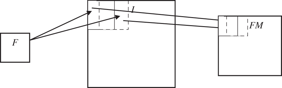
Figure 1: Feature map generation

Fig. 2 shows the computation of FM by a convolution filter F of size 3 × 3 to an input image of size 5 × 5 with a stride of 1. For simplicity, a simple convolution filter is assumed. The output of F to a specific window on the input image is shown in the FM with the same color.

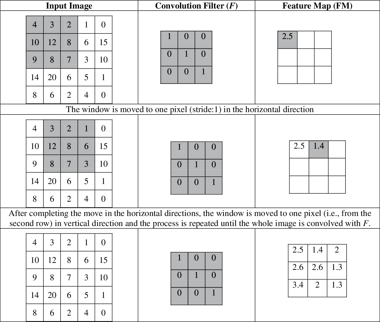
Figure 2: Example of a convolution layer in the architecture

The hierarchical decomposition is achieved by stacking of convolution layers i.e., the convolution layer also operates on the output of other layers to get more information from the input. The abstraction of features increases while increasing the depth of the network. The major difference between the modified VGG architecture and the conventional VGG is the logic behind the pooling layers. Fig. 3a shows the original VGG architecture with 16 weight layers and Fig. 3b shows the modified VGG architecture with the same number of layers. Fig. 4 shows the feature map obtained from the first convolution layer.

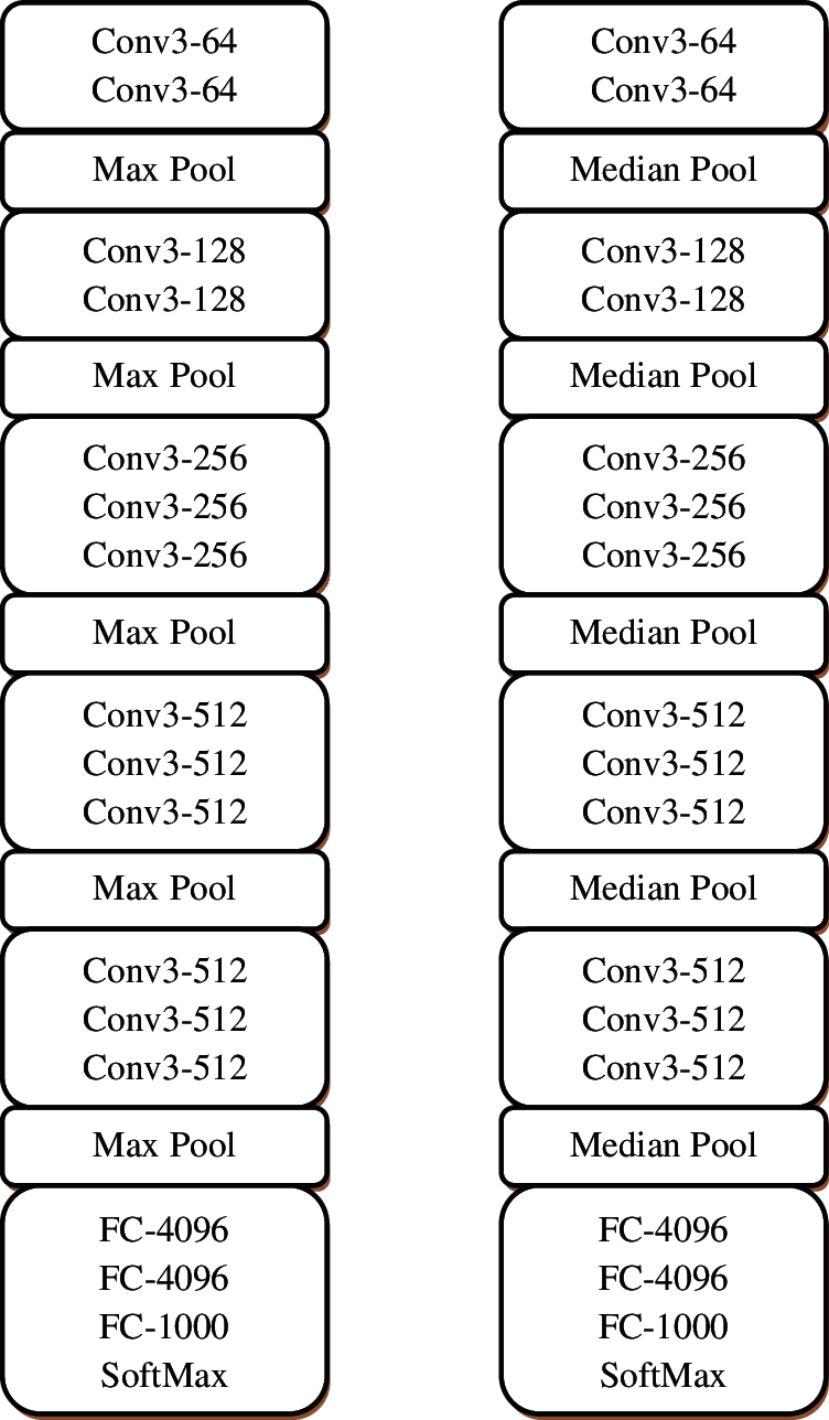
Figure 3: (a) Conventional VGG-16 architecture (b) Modified VGG-16 architecture

Figure 4: (a) Input image (b) Feature map (FM) from the first convolution layer of modified VGG-16 architecture

The feature maps from the convolution layer are down-sampled by pooling layers. The pooling operation is applied to the feature map with a predefined size of patches and stride. The movement over the pixels along vertical and horizontal directions between the successive applications of filters is referred to as stride and it is typically set to (2, 2). The common techniques used for down sampling are maximum pooling and average pooling. Let us consider a sample FM of size 2 × 6 in Eq. (1).

FM=[241128201133] (1)

The application of maximum pooling (Pmax) reduces the FM from 2 × 6 to 1 × 3 with a stride of (2, 2) and patches of (2 × 2). Thus, the first step is applied to the Pmax operation which is given below:

max[2420]=4 (2)

The next step is the application of stride, thus Pmax is applied on the FM by moving at left along the two columns,

max[1111]=1 (3)

This operation is continued until it reaches the last rows and last columns,

max[2833]=8 (4)

The final result of the Pmax is shown in Eq. (5)

Pmax=[418] (5)

Similarly, the application of average pooling (Pavg) is given in Eq. (6)

Pavg=[214] (6)

Instead of using the common pooling methods, the median pooling layer is introduced in the modified VGG architecture. The application of the median pooling layer (Pmed) is given in Eq. (7).

Pmed=[213] (7)

The main reason to use the median is that the median value is less affected by outliers than average or max. The outliers are observation which has abnormal distance from other samples in the population. Fig. 5 shows how the different pooling layers work in the architecture.

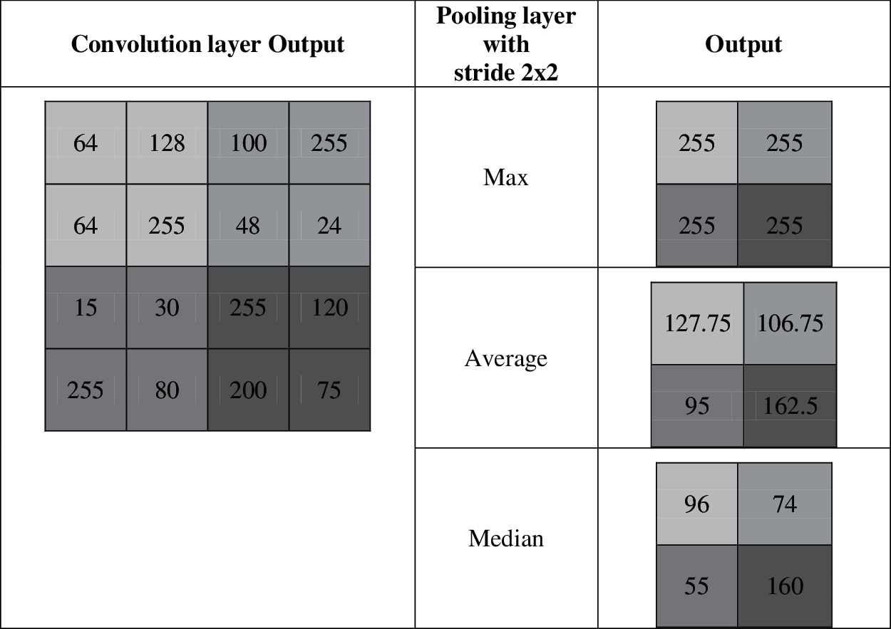
Figure 5: Example for different pooling layers

It is observed from Fig. 5 that the output of the max-pooling layer is affected by outliers and the output of the average pooling layer depends on the outliers. In this case, the median pooling layers are not affected by the outliers that may increase the performance of the system. In the hidden layers, rectified linear activation function is used which is defined as

ReLu(y)=max(0,y) (8)

After the operations on these layers, the final extracted FM is given to the output layer where the predictions will take via the softmax layer. It converts the output of the layer into a probability distribution for potential outcomes. It is defined by

SM(yi)=eyi∑jeyj (9)

where j is the total number of outputs from the last layer and yi is the output of the ith layer. From the probability distribution SM(yi) , the target class is assigned with the class which has a high probability. Though other activation functions such as tanh and sigmoid are available, this study uses softmax as other functions stuck while training the network. Also, the modified VGG architecture uses mini-batch gradient descent with momentum of 0.9 and stochastic gradient descent optimizer is employed. The number of epochs is set to 20 and cross entropy loss function is used. The computation of the softmax layer is shown in Tab. 1.

3  Results and Discussions

The superiority of the modified VGG architecture is demonstrated in this section. The REMBRANDT dataset [18–19] consists of MRI brain images of 130 patients which are downloaded freely [20]. The in-plane resolution of images is 256 × 256 pixels. The database consists of MRI images from normal and glioma patients. Samples from normal and abnormal images are shown in Fig. 6.

Figure 6: (a) Normal and (b) Abnormal

200 MRI images are randomly selected with 100 normal and 100 abnormal. The setting for database split-up for training and testing is shown in Tab. 2 which is used to evaluate the system.

For a supervised classification model, the network should be trained using known training samples before classification. At first, the available images (200) are divided into two sets; training (70%) and testing sets (30%). The VGG architectures are trained using the former set of images and then testing by the later set of images. As the raw pixels of an image are given to the modified VGG architecture, an input database is created at first which contains the raw pixels and output labels of all selected images from the REMBRANDT dataset. After successful training, the modified VGG architecture is implemented in the testing phase. In this phase, a test image is individually inputted to the system and the output class (+1 for abnormal and −1 for normal) is stored which is compared to the ground truth data to determine the correct classification. This process is repeated for all testing images in the input database and a confusion matrix is drawn based on the results which are shown in Tab. 3. In this table TP represents True Positive, TN represents True Negative, FP represents False Positive, and FN represents False Negative.

The efficiency of the system to categorize the test MRI brain images into two classes; P-cases or N-cases is measured based on the following performance metrics:

Accuracy: It gives the overall performance of the system for both normal and abnormal brain image classification accuracy.

Accuracy=TP+TNTP+FN+TN+FP (10)

Sensitivity: It shows the ability of the system to identify P cases correctly.

Sensitivity=TPTP+FN (11)

Specificity: It shows the ability of the system to identify N cases correctly.

Specificity=TNTN+FP (12)

Tab. 4 shows the performance metrics of the system presented in this study for brain image classification system.

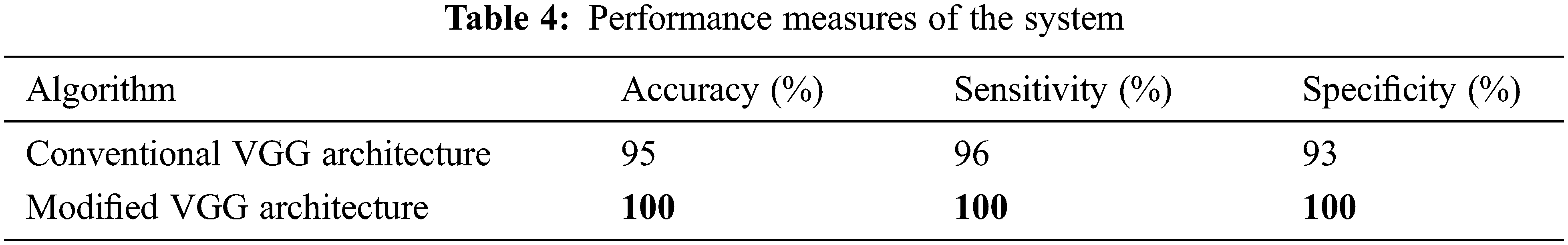
It is observed that the accuracy of conventional VGG architecture is low for brain image classification than modified VGG architecture. One of the reasons for the highest accuracy of modified VGG architecture is the application of median pool layers instead of the max-pooling layer which is less affected by outliers. Also, the robustness of conventional VGG architecture is limited as the accuracy changes for different iterations. Tab. 5 shows the performance comparison of modified VGG architecture when compared to recent brain image classification results using different features and classifiers.

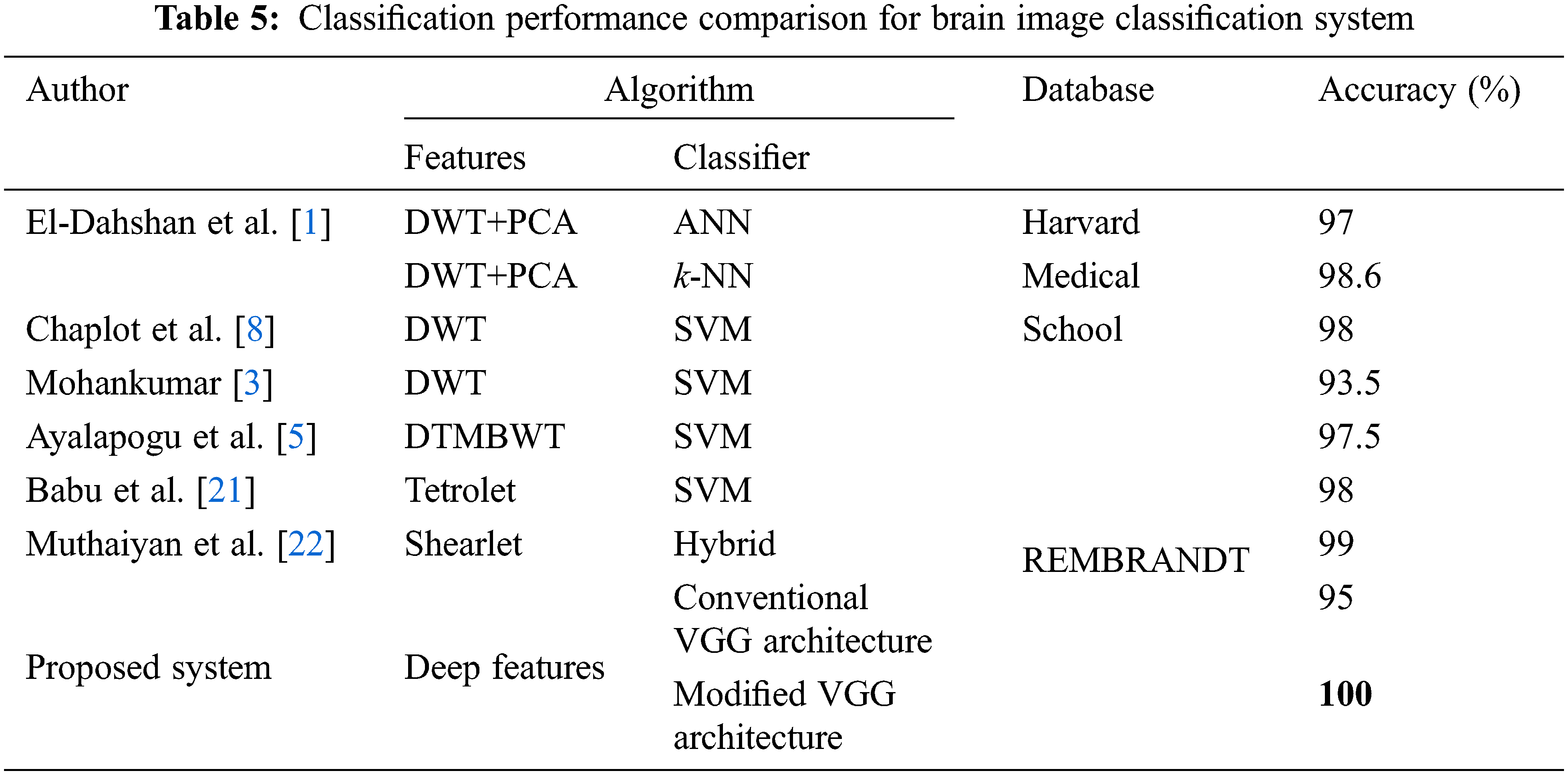
The references [4–5] had used different variants of wavelets such as DWT, dual tree M band WT (DTMBWT) respectively to perform feature extraction and utilized SVM for the classification approach. But they had achieved the classification accuracy of below 98%. Even though the results in [1–3,8] had achieved 100% accuracy, but they had used Harvard medical school images of a total of only 75 images. The Modified VGG architecture of the proposed system has attained classification accuracy of 100% for a total of 200 images which means that all test images from the REMBRANDT database are correctly classified. Hence from the performance comparison table, it is proved that the proposed architecture is more efficient than the compared references.

4  Limitations

The main limitation of this study is the small study population (200 images) which is randomly selected from REMBRANDT database. Also, the system is tested by using MRI images only. The modified VGG architecture can be evaluated using advanced validation techniques such as k-fold cross validation to confirm the efficiency of the system.

5  Conclusions

The ability of deep learning is utilized in this study to design a computer system for image classification. The conventional VGG architecture is modified to improve the analysis of medical images. It is applied to classify the REMBRANDT database images to a normal brain or an abnormal brain. Due to the visual similarity and huge intra-class variance between the brain images of normal and abnormal categories, it is not possible to manually classify them. The modified VGG architecture provides excellent performance in terms of classification accuracy, specificity, and sensitivity. Also, it is shown that a significant improvement of 5% over the conventional VGG architecture (95%) is obtained. This is due to that the median pooling layer reduces the dimension of deep features with almost no noisy features. Although the system is applied for only MRI brain images, it can be logically applied to other types of diseases also. In future, the median pooling layer can be integrated with other deep learning approaches such as AlexNet and GoogleNet and their performances will be analyzed for brain image classification.

Funding Statement: The authors received no specific funding for this study.

Conflicts of Interest: The authors declare that they have no conflicts of interest to report regarding the present study.

This work is licensed under a Creative Commons Attribution 4.0 International License, which permits unrestricted use, distribution, and reproduction in any medium, provided the original work is properly cited.

References

1. E. S. A. El-Dahshan, T. Honsy and A. B. M. Salem, “Hybrid intelligent techniques for MRI brain images classification,” Digital Signal Processing, vol. 20, no. 2, pp. 433–441, 2010. [Google Scholar]
2. M. Saritha, K. P. Joseph and A. T. Mathew, “Classification of MRI brain images using combined wavelet entropy based spider web plots and probabilistic neural network,” Pattern Recognition Letters, vol. 34, no. 16, pp. 2151–2156, 2013. [Google Scholar]
3. S. Mohankumar, “Analysis of different wavelets for brain image classification using support vector machine,” International Journal of Advances in Signal and Image Sciences, vol. 2, no. 1, pp. 1–4, 2016. [Google Scholar]
4. M. Maitra and A. Chatterjee, “A Slantlet transform based intelligent system for magnetic resonance brain image classification,” Biomedical Signal Processing and Control, vol. 1, no. 4, pp. 299–306, 2006. [Google Scholar]
5. R. R. Ayalapogu, S. Pabboju and R. R. Ramisetty, “Analysis of dual-tree M-band wavelet transform based features for brain image classification,” Magnetic Resonance in Medicine, vol. 80, no. 6, pp. 2393–2401, 2018. [Google Scholar] [PubMed]
6. K. Shankar, M. Elhoseny, S. K. Lakshmanaprabu, M. Ilayaraja, R. M. Vidhyavathi et al., “Optimal feature level fusion based ANFIS classifier for brain MRI image classification,” Concurrency and Computation: Practice and Experience, vol. 32, no. 1, pp. 1–12, 2018. [Google Scholar]
7. S. Ramathilagam, R. Pandiyarajan, A. Sathya, R. Devi and S. R. Kannan, “Modified fuzzy-means algorithm for segmentation of T1-T2-weighted brain MRI,” Journal of Computational and Applied Mathematics, vol. 235, no. 6, pp. 1578–1586, 2011. [Google Scholar]
8. S. Chaplot, L. Patnaik and N. Jagannathan, “Classification of magnetic resonance brain images using wavelets as input to support vector machine and neural network,” Biomedical Signal Processing and Control, vol. 1, no. 1, pp. 86–92, 2006. [Google Scholar]
9. M. K. Wali, M. Murugappan, R. B. Ahmad and B. S. Zheng, “Development of discrete wavelet transforms (DWT) toolbox for signal processing applications,” in Int. Conf. on Biomedical Engineering, Penang, Malaysia, pp. 211–216, 2012. [Google Scholar]
10. M. K. Bhuyan, Image descriptors and features. In: Computer Vision and Image Processing: Fundamentals and Applications, 1st ed., USA: CRC Press, pp. 85–105, 2019. [Google Scholar]
11. S. Ouchtati, J. Sequeira, B. Aissa, R. Djemili and M. Lashab, “Brain tumors classification from MR images using a neural network and the central moments,” in Int. Conf. on Advanced Systems and Electric Technologies, Hammamet, Tunisia, pp. 455–460, 2018. [Google Scholar]
12. S. Lahmiri, “Glioma detection based on multi-fractal features of segmented brain MRI by particle swarm optimization techniques,” Biomedical Signal Processing and Control, vol. 31, pp. 148–155, 2017. [Google Scholar]
13. A. Krizhevsky, I. Sutskever and G. E. Hinton, “Image net classification with deep convolutional neural networks,” in Advances in Neural Information Processing Systems, Cambridge, MA, USA, MIT Press, pp. 1097–1105, 2012. [Google Scholar]
14. K. Simonyan and A. Zisserman, “Very deep convolutional networks for large-scale image recognition,” in 3rd Int. Conf. on Learning Representations, San Diego, CA, USA, pp. 1–14, 2015. [Google Scholar]
15. C. Szegedy, W. Liu, Y. Jia, P. Sermanet, S. Reed et al., “Going deeper with convolutions,” in IEEE Conf. on Computer Vision and Pattern Recognition, Boston, MA, USA, pp. 1–9, 2015. [Google Scholar]
16. H. Mohsen, E. S. A. El-Dahshan, E. S. M. El-Horbaty and A. B. M. Salem, “Classification using deep learning neural networks for brain tumors,” Future Computing and Informatics Journal, vol. 3, no. 1, pp. 68–71, 2018. [Google Scholar]
17. H. H. Sultan, N. M. Salem and W. Al-Atabany, “Multi-classification of brain tumor images using deep neural network,” IEEE Access, vol. 7, pp. 69215–69225, 2019. [Google Scholar]
18. L. Scarpace, A. Flanders, R. Jain, T. Mikkelsen and D. W. Andrews, “Data from REMBRANDT. The cancer imaging archive,” [Online]. Available: http://doi.org/10.7937/K9/TCIA.2015.588OZUZB. [Google Scholar]
19. K. Clark, B. Vendt, K. Smith, J. Freymann, J. Kirby et al., “The cancer imaging archive (TCIAMaintaining and operating a public information repository,” Journal of Digital Imaging, vol. 26, no. 6, pp. 1045–1057, 2013. [Google Scholar] [PubMed]
20. REMBRANDT. [Online]. Available: https://wiki.cancerimagingarchive.net/display/Public/REMBRANDT. [Google Scholar]
21. B. S. Babu and S. Varadarajan, “Detection of brain tumour in MRI scan images using tetrolet transform and SVM classifier,” Indian Journal of Science and Technology, vol. 10, no. 19, pp. 1–10, 2017. [Google Scholar]
22. R. Muthaiyan and D. M. Malleswaran, “An automated brain image analysis system for brain cancer using Shearlets,” Computer Systems Science and Engineering, vol. 40, no. 1, pp. 299–312, 2022. [Google Scholar]
Cite This Article
Copyright © 2022 The Author(s). Published by Tech Science Press.