Automated White Blood Cell Disease Recognition Using Lightweight Deep Learning

1  Introduction

Clinical imaging is the strategy and interaction of making outline portrayals of the inside of a body [1–3] for clinical examination and clinical intercession. Clinical imaging tries to uncover inward designs covered up by the skin and bones [4–6], just as to analyze and treat infection. Medical images are frequently got to give the procedure of tactics that Non-invasively produce images of the internal part of the human body [7,8]. In the limited sense, the clinical images can be viewed like the arrangements of numerical back problems [9,10]. This implies that reason emerges as a result of the effect (the noticed sign). According to a clinical ultrasound account, the test consists of ultrasonic pressing force waves and repeats that go through tissues to reveal the underlying structure. Red blood cells, platelets, and white blood cells make up the majority of the cells in the blood [11]. White Blood cells likewise take significant capacities used for the insusceptible framework and are the primary guard of body against contaminations and diseases [12,13]. There are many types of white blood cells as illustrated in Fig. 1. In United States (USA), one person is diagnosed every three minutes with leukemia or myeloma. In year 2021, estimated 186,400 peoples are diagnosed with leukemia. Every 9 min, one person is died with blood cancer in US. Due to blood cancer, the estimated deaths in year 2021 are 57,750 [14].

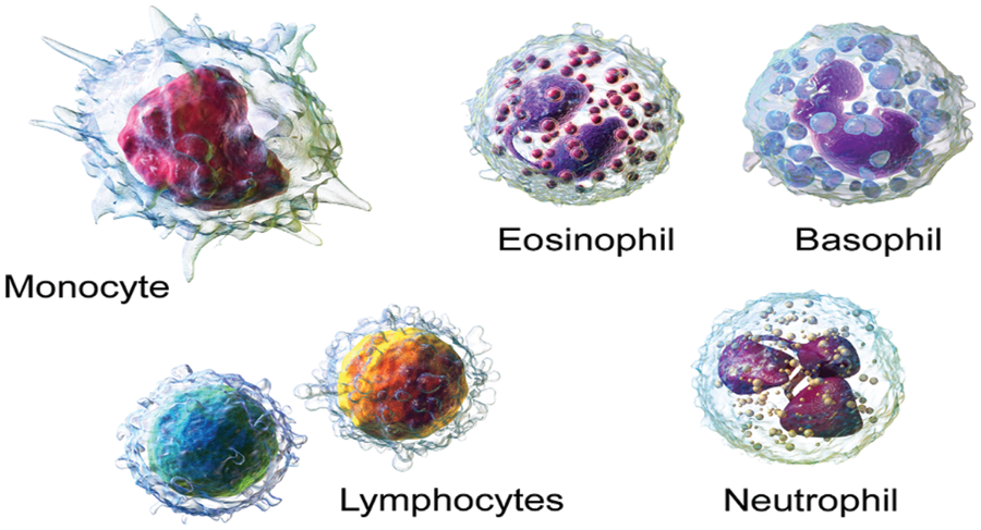
Figure 1: Types of WBC [30]

Monocytes: They have a more extended lifecycle than many of the white blood cells (WBC) and it help to breakdown the bacteria [15–17].

Lymphocyte: They make antibodies to battle against microbes, infections, and other possibly destructive trespassers [18–20].

Neutrophils: They eliminate and digest bacteria and fungi. They are the most various kind of WBC and your first line of safeguard when contamination strikes [21–23].

Basophils: These little cells appear to sound a caution when irresistible specialists attack your blood. They emit synthetic substances like histamine, a marker of unfavorably susceptible infection, that assist with controlling the body’s immune response [24–26].

Eosinophils. They assault and kill parasites and cancer cells and help with unfavorably susceptible reactions [27–29].

The classification of WBC diseases from images is a common task. Manual inspection is a time-consuming and stressful process. As a result, computerized techniques are widely required, and many techniques used in the literature are based on some important steps such as preprocessing of original images, features engineering, feature reduction or optimization, and finally classification [31]. Traditional computer based techniques also used segmentation to obtain more informative features, but the addition of middle steps always increases a system’s computational time. Furthermore, the manual feature extraction process did not perform well when the available dataset size was large and complex in nature [32].

Deep learning recently demonstrated outstanding performance for classification tasks in a variety of applications, including object detection [33], agriculture [34], medical imaging [35,36], surveillance [37], and a few others [38,39]. Deep learning is used in the medical domain for skin lesion classification [40,41], brain tumor classification, lung cancer classification [42], covid classification [43], and stomach disease classification [44]. As mentioned in [45], the authors have tackled with the issue of identifying white blood cells. With the help of a feed-forward neural network, they have classified the white blood cells into 5 classes. At first, blood cells were segmented from the microscopic images. Then, the neural network was fed, 16 of the most important features of the cells as input. After the segmentation, half of the images obtained, out of 100, were used to train the neural network, while the other half was used for testing purpose. In [46], the authors presented a sequential deep learning framework in order to identify and classify white blood cells into their 4 types. For the pre-processing phase, this study has offered three successive calculations. These calculations are named as, bounding box distortion, color distortion and image flipping mirroring. In the next step, Inception and ResNet models are used to perform feature extraction of the white blood cells. In [47], the authors have proposed a technique called Leishman-stained multi directional transformation-invariant deep classification (LSM-TIDC), to tackle the issue of white blood cells classification. The authors have used this method due to the fact that it utilizes interpolation and Leishman-stained function because they not only removed false areas of several input images but also they need no special segmentation. In the next step, multi-directional feature extraction is applied on the preprocessed images for the optimal and relevant feature extraction. By implementing transformation invariant model, in order to detect and classify blood cells, a system is designed shown in Fig. 2. As a result, the nucleus is extracted and then the system performs classification by applying convolutional and pooling properties of the system. Wang et al. [11] presented an three dimensional (3D) attention module for white blood diseases classification. The presented method extracted the spatial and spectral features instead of single type features and shows improved performance of 97.72%. Khan et al. [48] presented an automated framework for white blood diseases classification using classical features selection and extreme learning machine (ELM). They initially performed augmentation process through pixel stretch technique and then extract some classical features. Further they opted a maximum relevance approach for redundant features reduction. At the end, they used ELM for final classification. They used two datasets and achieved an improved accuracy of 96.60%.

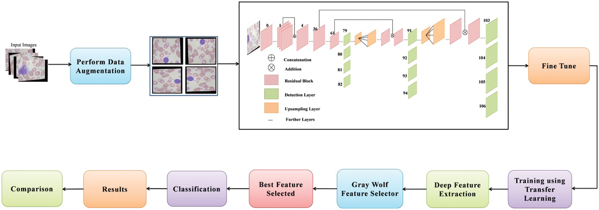
Figure 2: Proposed deep learning and optimization of features based architecture for white blood diseases classification

However, for WBC illness categorization, there are a few strategies that use deep learning. Furthermore, to our knowledge, there is no technique for optimizing deep learning features for WBC illness categorization. The main goal of optimization is to extract the best features from the generated deep learning features in order to improve classification accuracy while saving time. Convolutional layers, pooling layers to alleviate the problem of overfitting, activation layers, normalization layers, fully connected layer, and a SoftMax classifier are all common layers in a simple deep learning model. A few researchers start from scratch with a pre-trained model, while others freeze some layers and train using transfer learning. However, each phase has its own set of difficulties.

The following issues for WBC disease classification have been discussed in this article: i) In comparison to deep learning, traditional image processing techniques are slow and inaccurate; ii) Manual classification is a difficult process due to a number of factors, including time consumption, the availability of an expert, and the experience of an expert; iii) In the traditional technique, they must first extract the region of interest (ROI) and then extract feature, which is time consuming and increases the chance of classification error; and iv) the presence of irrelevancies. In this work, our main objective is to performed data augmentation and obtained a better trained model for accurate WBC diseases classification. Our major contributions in this work are listed as follows:

• Balance the imbalance classes using data augmentation, whereas the selected operations are flipping horizont on al and vertical directions.

• Modified a pre-trained deep learning model and freeze 50% layers. The fine-tuned model is later trained through transfer learning and performed features engineering on average pooling layer.

• A hybrid binary gray wolf optimizer algorithm is developed based on fixed ratio for the selection of best features. The neural network is employed as a fitness function instead of fine-K nearest neighbor (Fine-KNN).

The rest of the manuscript is organized in the following order. Section 2 of this manuscript is presented the proposed methodology. Results and detailed discussion added under Section 4. Finally, Section 5 conclude the manuscript.

2  Proposed Methodology

This section outlines the proposed deep learning-based methodology for classifying white blood cell disorders. The suggested framework’s architecture is represented in Fig. 2. Data augmentation is done on the original photos first, then sent to the DarkNet53 deep network, which has been fine-tuned for training. The model is trained via transfer learning. After that, the trained model is used to extract features from the global average pool layer. After that, a reformed grey wolf optimization algorithm is used to select the best features. For the selection process, the number of iterations can be 50, 100, 150, or 200. Machine learning classifiers are used to classify the best picked features, and the results are acquired.

2.1 Dataset Description

In this work, we combined two datasets–LISC and Dhruv for the experimental process [49]. The selected datasets consists of four types of WBC diseases such as Eosinophil, Lymphocyte, Monocyte, and Neutrophil, as illustrated in Fig. 3. Initially, the images in these datasets are limited and not enough to train a deep learning model; therefore, we applied augmentation step to increase the number of images for better training of a deep learning model. Three different operations are applied on each class such as horizontal flip, vertical flip, and transpose. Mathematically, these operations are defined as follows:

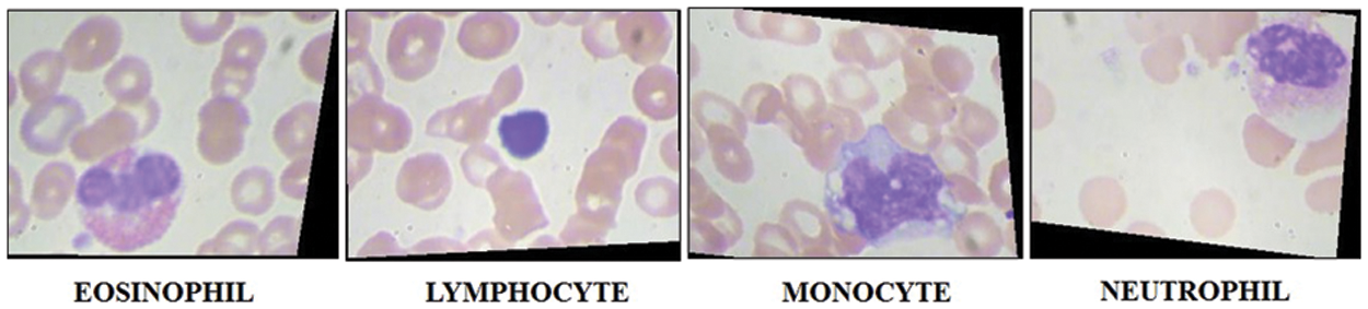
Figure 3: Sample images of WBC imaging dataset

Consider Δ represents the entire images database, λ(x,y) represents each image in the database having dimension 256×256×k , where k=3 . On each image λ(x,y) , three operations are applied such as horizontal pixels movement, vertical pixels movement, and transpose. Mathematically, these operations are defined as:

λh(x,y)=λ(x+1−y) (1)

λv(x,y)=λ(y+1−x) (2)

λt(x,y)=λyx (3)

where, λh(x,y) represents horizontal pixels movement operation, λv(x,y) represent vertical pixels movement operation, and λt(x,y) represent pixels transpose. After these operations, the number of images in each class increases to 4000 which are previously below 500. A few sample images are illustrated in Fig. 4.

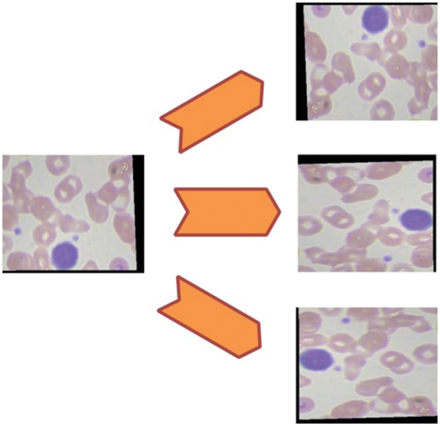
Figure 4: Representation of data augmentation step

2.2 Modified Darknet-53 Model Features Extraction

Darknet is a neural network framework that is free and open source. It is a quick and highly accurate framework for real-time object detection (accuracy for specific trained models is dependent on training data, epochs, batch size, and other factors) and used for input images. The principal feature extraction module of the real-time object detection network you only look once (YOLOv3) is Darknet-53, which was introduced in 2018. The goal of Darknet-53 is to extract characteristics from input photos. YOLO version 3 implements a 53-layered fully convolutional architecture with successive 3 × 3 and 1 × 1 fully connected layers for feature extraction. The structure of modified Darknet-53 model is shown in Fig. 5.

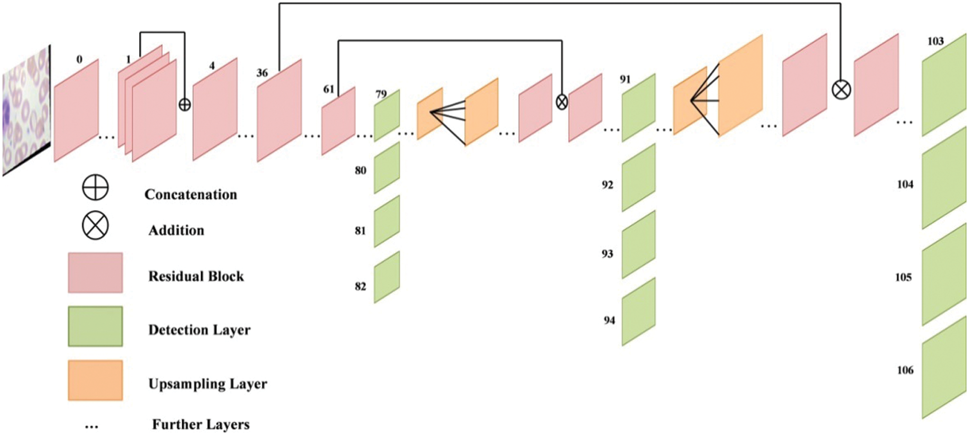
Figure 5: Structure of modified darknet-53 model

For detecting purpose, 53 additional layers are added, giving YOLO v3 a 106-layer convolutional architecture. After each convolution layer, the batch normalization (BN) layer and the LeakyRelu layer are utilized. The name of this network architecture framework is Darknet-53. To determine the classes that the boundary box may contain, YOLOv3 uses a separate logical classifier with a multi-label classification for every prediction box. The network topology is expanded to layer 53 using continuous 3 × 3 and 1 × 1 convolutional layers. In terms of prediction methodologies, YOLOv3 predicts three border boxes for each panel.

The convolutional neural network (CNN) uses convolution instead of regular matrix multiplication in at least one layer, as indicated in Eq. (4). Convolution also permits for different input sizes. It is a mathematical process that inputs two functions x(i) , and y(i) , and generates a third function that demonstrates how the shape of one of the functions affects the shape of the other.

g(i)=(x∗y)(i)=∫−∝∝⁡x(i)y(i−Δ)lΔ (4)

Sparse interaction, equivalent modeling and parameter sharing are three principles that CNN layers are constructed on. The term “sparse interaction” refers to the network’s kernel size being smaller than the size of input. This makes the network much more efficient because the matrix multiplication technique is an O(nm) process, where the input size is denoted by n and the output size is denoted by m. Parameter sharing derives from the fact that parameters in a CNN are reused in a way that they aren’t in traditional artificial neural network (ANN). It really has no impact on the running time, but it does reduce the amount of memory used, which is critical in large CNNs. Convolutional layers, like ReLU, have both a multiplication and a non-linear input vector. In most cases, the CNN has more than one pooling layers. A pooling layer is a type of layer that takes a large input and reduces it to a smaller size. This is accomplished by selecting the mean or highest value of subsampled squares inside the input. The important layer in the CNN architecture is fully connected layer. It connects all of the active spots in the layers that came before it. Its output is an n -dimensional vector, where n denotes the number of classes for which the network has been trained. We have four classes in our research. The likelihood that the object relates to the class is represented by each member in the vector. The categorization result is the element with the maximum probability. The architecture of CNN is shown in Fig. 6.

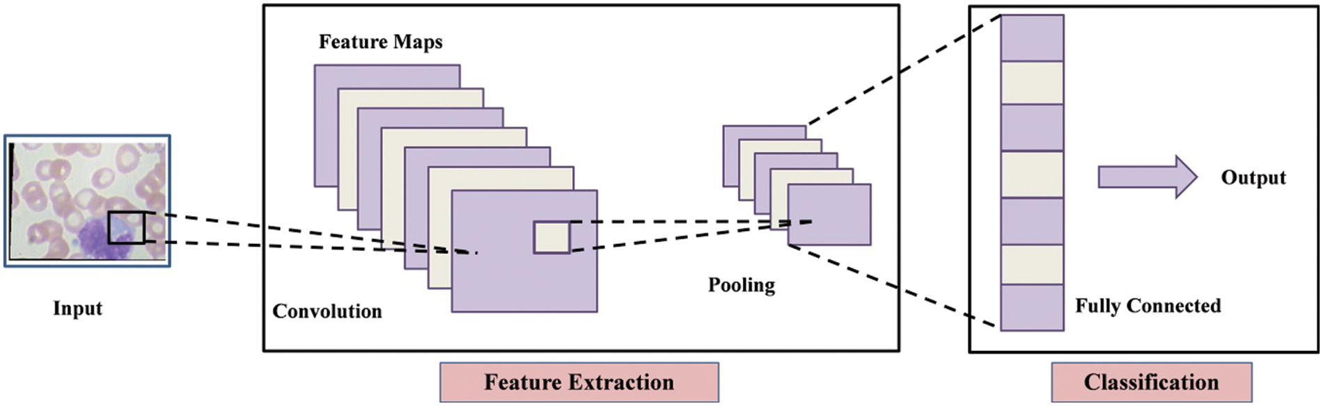
Figure 6: Architecture of convolutional neural network (CNN)

The above model is fine-tuned and added few new layers and trained through transfer learning (TL) [50]. Visually, the working of TL process is illustrated in Fig. 7. Mathematically, the TL is described as follows:

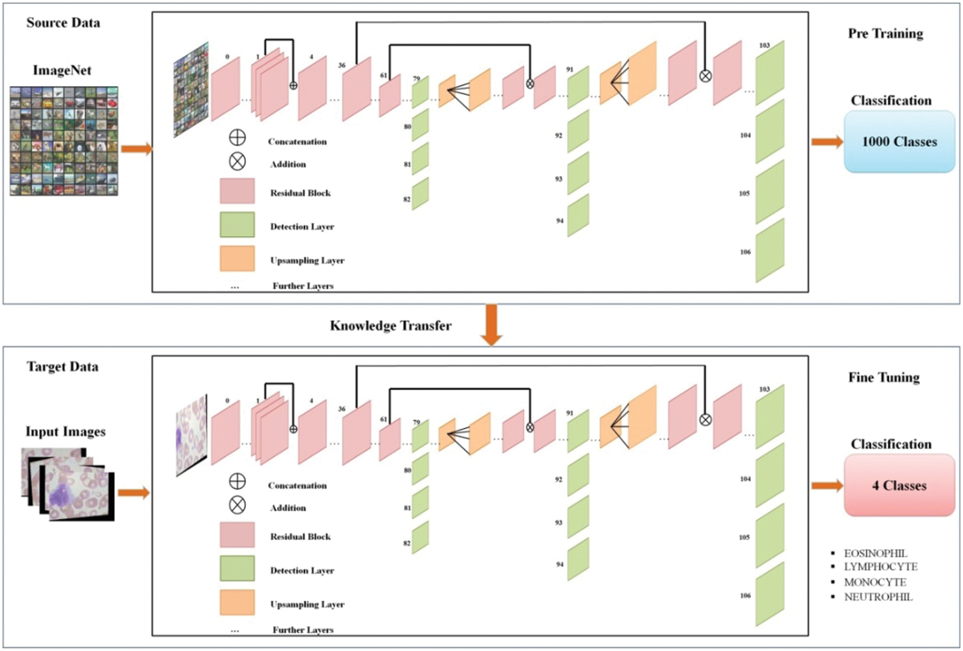
Figure 7: Representation of transfer learning

Transfer learning worked to increase the learning of the target predictive function fTp() in Td using the knowledge in Sd and Tsl , where Sd≠Td or Tsl≠Ttl , given a source domain Sd and learning task Tsl , and a target domain Td and learning task Ttl .

A domain is defined as the pair d=V,f(V) in the specification above. As a result, the criterion Sd≠Td implies that VS≠Vt or ft(V)≠fs(V) .

A task is also described as a pair t=U,f(U|V) . As a result of the constraint Tsl≠Ttl , either Us≠Ut or f(Us|Vs)≠f(Ut|Vt) applies.

The learning problem becomes a conventional machine learning problem when the target and source domains are about the same, that is Sd=Td , and their learning tasks are the same, that is Tsl=Ttl .When the domains are dissimilar, one of two things can happen:

The feature spaces are distinct between the domains, that is VS=Vt .

The feature spaces are the same between domains, but the marginal probability distributions between domain data are not; that is f(Vs)=f(Vt) , where Vsi∈Vs and Vti∈Vt .

After the training of fine-tuned models, the activation is applied on global average pooling layer and extract features. The dimension of extracted features of this layer is M×1280 . The extracted features are analyzed and found some redundant information that need to be remove before final classification.

2.3 Best Feature Selection

Feature Selection is the process of minimizing the number of input variables. The set of input variables should be reduced to lower the computation complexity of modeling and, in some situations, to increase the model’s performance. Data redundancy is eliminated through feature selection step. In this work, we utilized an improved optimization algorithm named reformed gray wolf for best feature selection. After applying the improved gray wolf optimization algorithm, the original deep extracted feature vector is reduced to M×435 , where M represents the number of images utilized in the testing process.

To dynamically search the feature map for the optimal feature combination, the binary gray wolf optimization is applied. The various feature reducts for a feature vector of size n would be 2n , which is a big space of features to be explored accurately. The feature combination with the best classification performance and the fewest number of selected features is the best. Equation shows the fitness function being used binary gray wolf optimization to assess specific gray wolf placements.

fitnessfunction=∂δL(S)+ρ|N−L|N (5)

where δL(S) is the classified quality of condition characteristic set L similar to decision S, L is the length of the selected subset of features, N is the total numbers of features, and ∂∈[0,1] and ρ=1−∂ are two parameters related to the prominence of classification performance and subset length. The function of fitness improves classification quality ∂δL(S) , and the ratio of randomly selected features to total features |N−L|N . By using error rate instead of classification quality and selected feature ratio instead of unselected feature size, the preceding equation can simply be transformed into a sub problem.

fitnessfunction=∂ϵL(S)+ρ|L|N (6)

where ϵL(S) is the condition attribute set classifier’s error rate, the length of the selected feature subset is denoted by L, and the total number of features is represented by N.

For the feature selection challenge, a novel binary grey wolf optimization (bGWO) is presented in this work. The updating equation for wolves is based on three position vectors. Particularly vτ,vφ,vω which pulls each wolf to the first three optimal solutions. The pool of possibilities in the bGWO is binary at all times; all solutions are on the edge of a hypercube.

The major modifying equation in the bGWO technique could be written as follows: The τ is a fittest solution in the mathematical model for the grey wolf optimization (GWO). φ and ω are the names of the second and third best solutions, respectively. ∃ is considered for the remaining possible solutions. The hunt is led by τ,φ,ω and ∃ and these three candidates are followed. Before the pack can hunt a victim, it must first encircle it. The following formulations are used to mathematically model encircling behavior.

v¯(k+1)=vq¯(k)+H¯.J¯ (7)

where J¯ is described as in equation

J¯=|G¯.vq¯(k)−v¯(k)| (8)

Coefficient of vectors are presented by H¯ and J¯ . And the positions of the gray wolf and the prey denoted by v¯ and vq¯ respectively. The values of H¯ and G¯ are computed by the following equations.

H¯=2c.e1¯−c (9)

G¯=2e2¯ (10)

where c decreases gradually from 2 to 0 over iterations and e1¯ , e2¯ are random vectors in the range [0, 1]. The initial top three candidate solutions produced thus far force the remaining search agents (including the ∃ ) to update their locations in accordance with the best search agent’s positions. As a result, the wolves’ positions are updated as follows:

v¯(k+1)=v1¯+v2¯+v3¯3 (11)

where v1¯ , v2¯ , and v3¯ can be determined by the following equations:

v1¯=|vτ¯−H1¯.Jτ¯| (12)

v2¯=|vφ¯−H2¯.Jφ¯| (13)

v3¯=|vω¯−H3¯.Jω¯| (14)

where the first three best solutions are denoted by vτ¯ , vφ¯ and vω¯ . H1¯ , H2¯ and H3¯ are described in equation. And Jτ¯ , Jφ¯ and Jω¯ can be determined by following equations:

Jτ¯=|G1¯.vτ¯−v¯| (15)

Jφ¯=|G1¯.vφ¯−v¯| (16)

Jω¯=|G1¯.vω¯−v¯| (17)

The updating of the parameter c, which manages the ratio between exploration and exploitation, is a final note regarding the gray wolf optimizaation (GWO). According to the Eq. (18), the parameter is linearly modified on every iterations to ranging from 2 to 0.

c=2−k2maxiter (18)

Only the modified gray wolf position vector is constrained to be binary in this approach shown in Eq. (19).

vak+1={1ifsigmOid(v1+v2+v33)≥random0Otherwise (19)

where random numbers are chosen from the uniform distribution that is belong to binary numbers 0 and 1. vak+1 is representing the new binary location in dimension a at iteration k and sigmOid(o) is described as follows:

sigmOid(o)=11+σ−10(v−0.4) (20)

Finally, a best selected feature vector is obtained of dimension N×435 . The final selected features are classified using machine learning classifiers for classification. Several classifiers are employed in this work such as support vector machine (SVM), Fine KNN, ensemble trees, and neural network.

3  Results and Comparison

The experiments performed on the best selected testing features after four different feature sets such as: i) Classification using best selected features at 50 iterations; ii) Classification using best selected features at 100 iterations; iii) Classification using best selected features at 150 iterations, and iv) Classification using best selected features at 200 iterations. The augmented dataset has four classes such that Eosinophil, Lymphocyte, Monocyte and Neutrophil. Several classifiers are opted for the classification results and neural network gives better performance. The results are computed with ratio 50:50 and cross validation was 10. Several evaluation measures are employed such as sensitivity rate, precision rate, F1-Score, and accuracy. The time of each classifier is also opted for the experimental process. All the simulations of the proposed framework are conducted on MATLAB2021a using Intel Core i7 7700 processor, 8 GB of RAM, and an Intel HD Graphics 630 graphics processing unit (GPU).

3.1 Experiment No.1

The results of the first experiment are presented in Table 1. In this experiment, 50 numbers of iterations are performed and obtained the best feature vector for classification results. In this table, eight different classifiers performance has been discussed in terms of accuracy, sensitivity rate, time, and named a few more. The highest accuracy of 99.6% is obtained for neural network (NN), whereas the sensitivity rate is 99.70, precision rate is 99.65, F1-Score is 99.67, false negative rate (FNR) is 0.30, and classification time is 9.261 (s). These values can be further verified through a confusion matrix, illustrated in Fig. 8. The rest of the classifiers such as medium Gaussian SVM (MGSVM), cubic SVM (CSVM), Medium K Nearest Neighbor (MKNN), weighted KNN (WKNN), quadratic SVM (QSVM), cubic KNN (CuKNN), and cosine KNN (CoKNN) also achieved better accuracies of 98.4%, 98.4%, 98.1%, 98.6%, 97.5%, 97.5%, and 98.2%, respectively. The computational time of each classifier is also noted during the classification process and based on this table, it is observed that the minimum noted time is 9.261 (s) for NN.

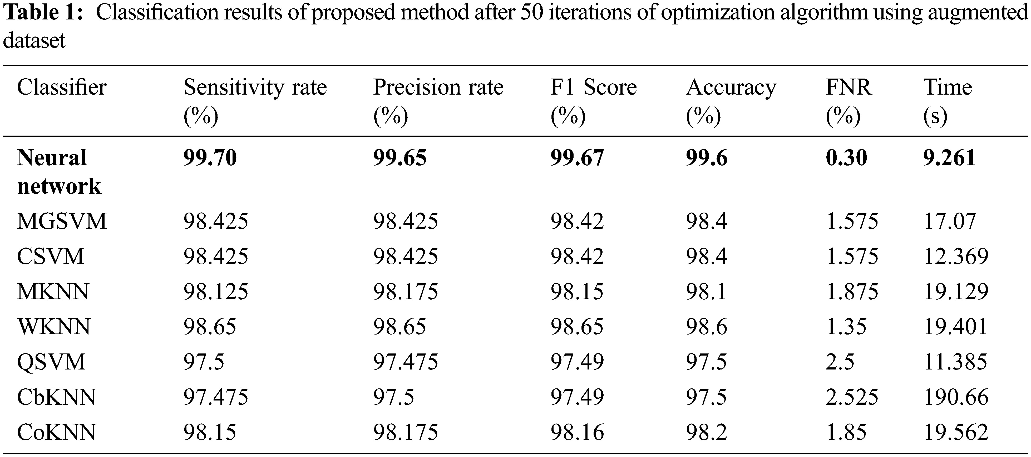
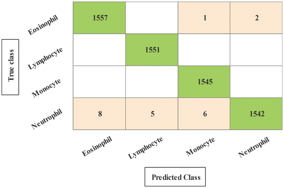
Figure 8: Confusion matrix of neural network for experiment 1

3.2 Experiment No.2

The results of the second experiment are presented in Table 2. In this experiment, 100 numbers of iterations are performed and obtained the best feature vector for classification results. The highest accuracy of 99.7% is obtained for neural network (NN), whereas the sensitivity rate is 99.75, precision rate is 99.75, F1-Score is 99.77, FNR is 0.25, and classification time is 12.602 (s). These values can be further verified through a confusion matrix, illustrated in Fig. 9. The rest of the classifiers such as medium Gaussian SVM (MGSVM), cubic SVM (CSVM), Medium KNN (MKNN), weighted KNN (WKNN), quadratic SVM (QSVM), cubic KNN (CuKNN), and cosine KNN (CoKNN) also achieved better accuracies, as listed in Table 2. The computational time of each classifier is also noted during the classification process and based on this table, it is observed that the minimum noted time is 12.602 (s) for NN. Moreover, the other classifier also not consumes more time but after the number of iterations, a little time is increased due to more numbers of feature selections.

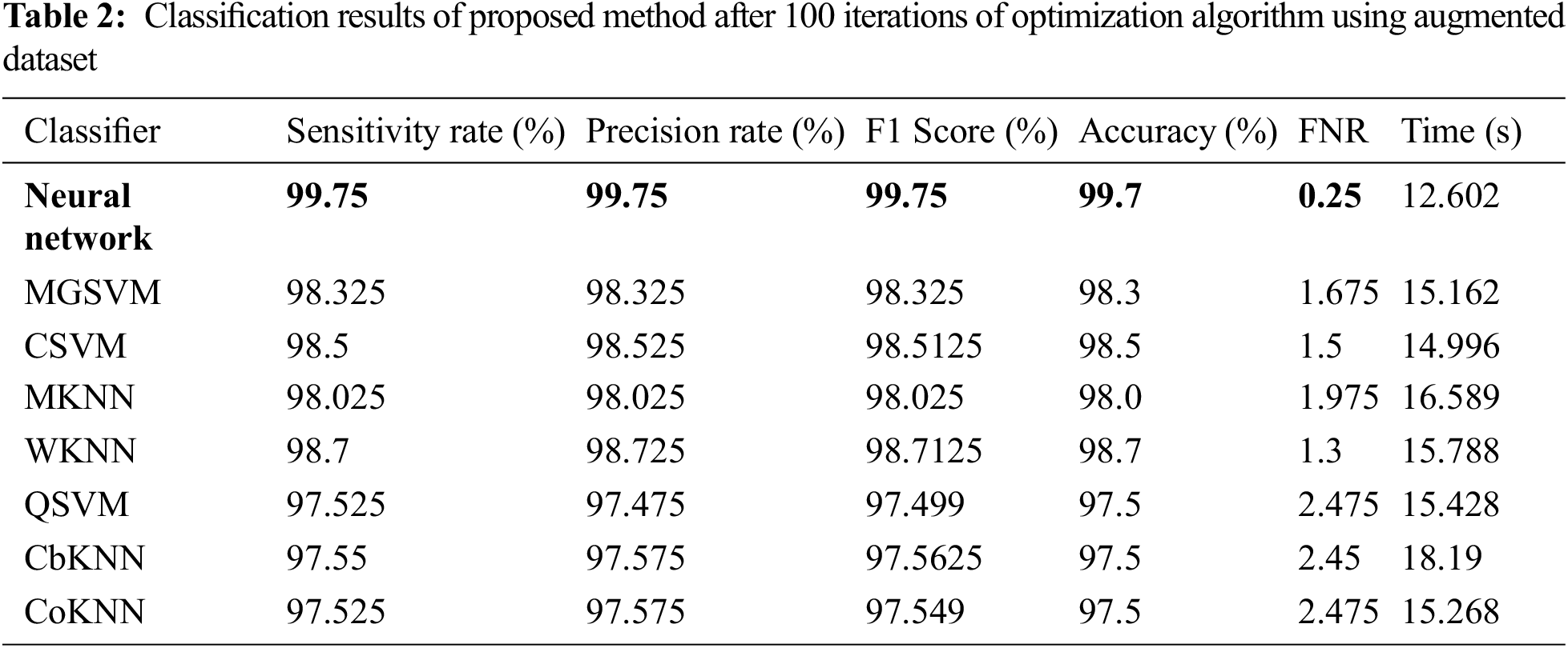
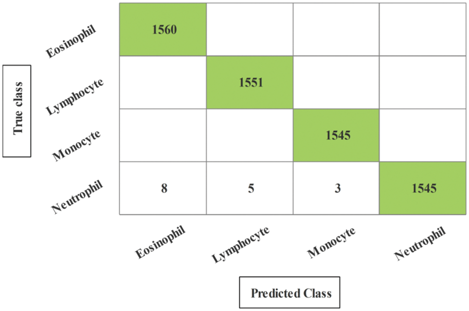
Figure 9: Confusion matrix of neural network for experiment 2

3.3 Experiment No.3 and 4

The results of the third and fourth experiments are presented in Tables 3 and 4. In these experiments, 150 and 200 numbers of iterations are performed and obtained the best feature vector for classification results. Table 3 presents the classification results of 3rd experiment and obtained the best accuracy of 99.6%, whereas the classification time is 15.39 (s). The confusion matrix of neural network (NN) for this experiment is also illustrated in Fig. 10. Through this figure, the sensitivity, precision, and F1-Score can be verified. Furthermore, the result of experiment four are given in Table 4 and obtained the best accuracy of 99.5%. This accuracy can be verified through a confusion matrix, illustrated in Fig. 11. In this experiment, the minimum noted computational time is 15.39 (s) that is little higher than the above three experiments. Overall, the experiment 2 gives the better accuracy of 99.7% and based on the time, experiment 1 is better.

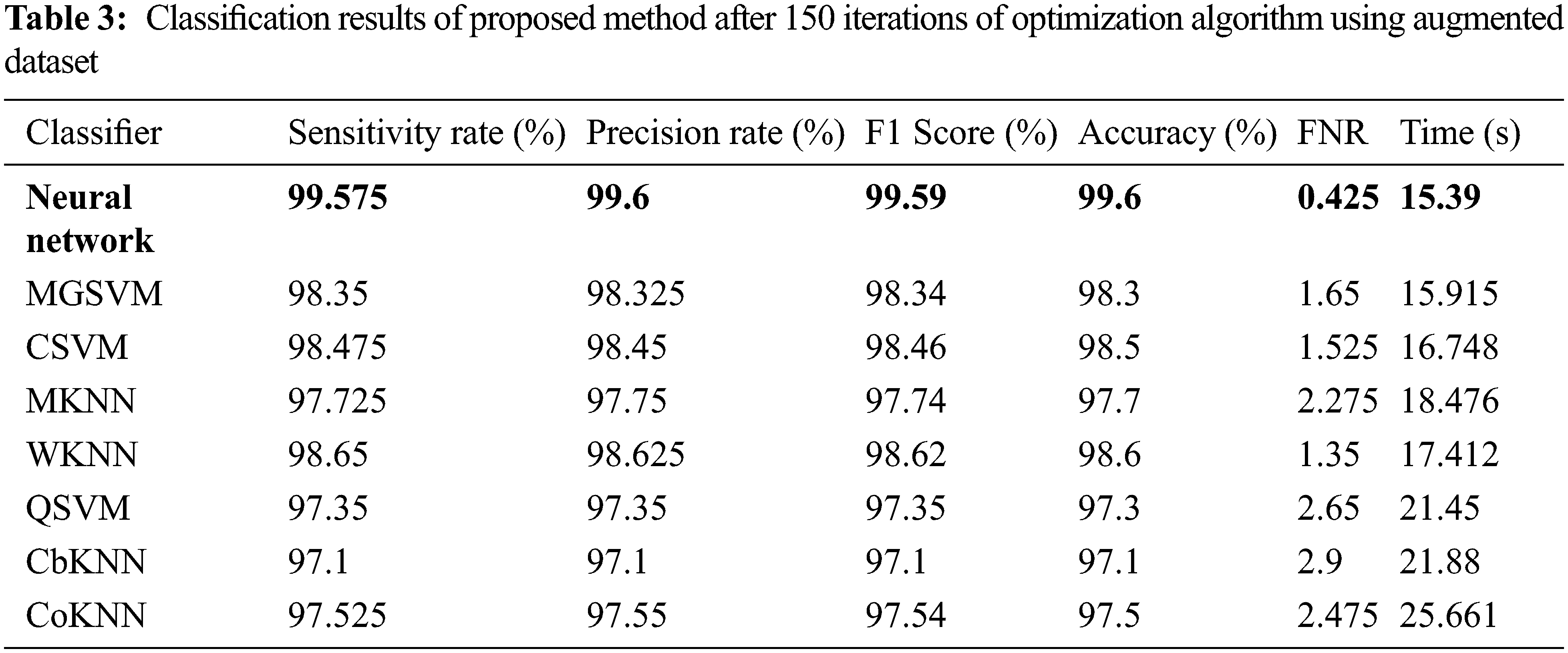
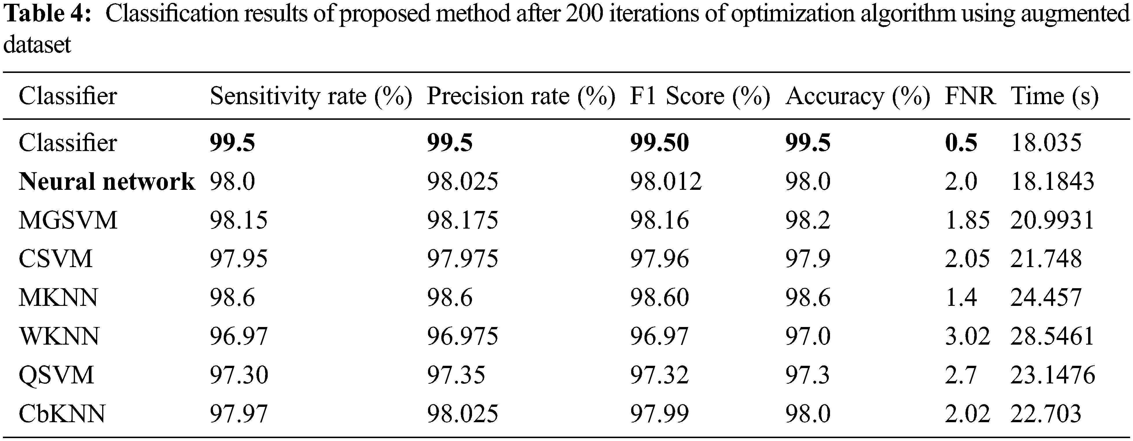
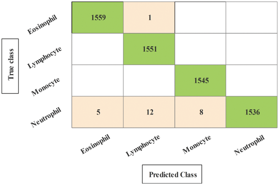
Figure 10: Confusion matrix of neural network for experiment 3

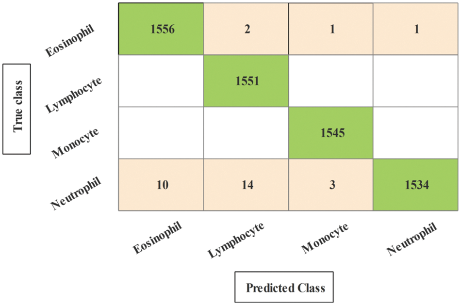
Figure 11: Confusion matrix of neural network for experiment 4

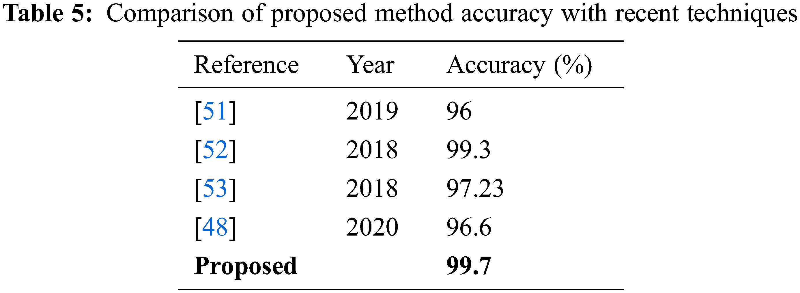
Comparison: The fine-tuned Darknet-53 deep learning model is utilized in this work for features extraction that later optimized using improved optimization algorithm. For the best feature selection, the optimization procedure is repeated with a different number of iterations such as 50, 100, 150, and 200. The results of each experiment are given in Tables 1–4 and confusion matrixes are illustrated in Figs. 8–11. Based on the results, NN gives better accuracy of 99.7% for 100 iterations. Moreover, the proposed method accuracy is also compared with some recent techniques, as presented in Table 5. In this table, it is observed that the proposed method accuracy is better than the recent techniques.

4  Conclusion

A deep learning and features optimization based technique for WBC illness categorization is proposed in this study. By conducting a data augmentation phase, the size of the selected dataset was enlarged, which was then used to train a pre-trained deep model. Using an upgraded optimization technique known as improved binary grey wolf optimization, features are retrieved and the best of them are chosen. After multiple iterations, features are chosen and a neural network is used to make the final classification. The NN achieved the best accuracy of 99.7% for 100 iterations on the supplemented dataset. Based on the results, it is concluded that the augmentation process improved the accuracy but increased the time that was reduced through selection technique. Moreover, the numbers of iterations increases the length of selected feature vectors that only affects the classification time. In the future, more datasets shall be considered and train some deep learning models from the scratch.

Funding Statement: This research project was supported by the Deanship of Scientific Research, Prince Sattam Bin Abdulaziz University, KSA, Project Grant No. 2021/01/18613.

Conflicts of Interest: The authors declare that they have no conflicts of interest to report regarding the present study.

References

 1.  N. A. Rudd and S. J. Lennon, “Body image and appearance-management behaviors in college women,” Clothing and Textiles Research Journal, vol. 18, no. 2, pp. 152–162, 2000. [Google Scholar]

 2.  R. L. Beard, “In their voices: Identity preservation and experiences of Alzheimer’s disease,” Journal of Aging Studies, vol. 18, no. 1, pp. 415–428, 2004. [Google Scholar]

 3.  A. V. Naumova, M. Modo, A. Moore and J. A. Frank, “Clinical imaging in regenerative medicine,” Nature Biotechnology, vol. 32, no. 5, pp. 804–818, 2014. [Google Scholar]

 4.  Z. Fayad and V. Fuster, “Clinical imaging of the high-risk or vulnerable atherosclerotic plaque,” Circulation Research, vol. 89, no. 7, pp. 305–316, 2001. [Google Scholar]

 5.  B. E. Bouma and G. Tearney, “Clinical imaging with optical coherence tomography,” Academic Radiology, vol. 9, no. 5, pp. 942–953, 2002. [Google Scholar]

 6.  N. Madan and P. E. Grant, “New directions in clinical imaging of cortical dysplasias,” Epilepsia, vol. 50, no. 2, pp. 9–18, 2009. [Google Scholar]

 7.  L. M. Broche, P. J. Ross, G. R. Davies and D. J. Lurie, “A whole-body fast field-cycling scanner for clinical molecular imaging studies,” Scientific Reports, vol. 9, no. 8, pp. 1–11, 2019. [Google Scholar]

 8.  R. Acharya, W. L. Yun, E. Ng, W. Yu and J. S. Suri, “Imaging systems of human eye: A review,” Journal of Medical Systems, vol. 32, no. 6, pp. 301–315, 2008. [Google Scholar]

 9.  H. D. Cavanagh, W. M. Petroll, H. Alizadeh, Y. G. He and J. V. Jester, “Clinical and diagnostic use of in vivo confocal microscopy in patients with corneal disease,” Ophthalmology, vol. 100, no. 11, pp. 1444–1454, 1993. [Google Scholar]

10. S. R. Arridge and M. Schweiger, “Image reconstruction in optical tomography,” Philosophical Transactions of the Royal Society of London. Series B: Biological Sciences, vol. 352, no. 21, pp. 717–726, 1997. [Google Scholar]

11. Q. Wang, J. Wang, M. Zhou, Q. Li and J. Chu, “A 3D attention networks for classification of white blood cells from microscopy hyperspectral images,” Optics & Laser Technology, vol. 139, no. 76, pp. 106931, 2021. [Google Scholar]

12. M. B. Terry, L. Delgado-Cruzata, N. Vin-Raviv and R. M. Santella, “DNA methylation in white blood cells: Association with risk factors in epidemiologic studies,” Epigenetics, vol. 6, no. 7, pp. 828–837, 2011. [Google Scholar]

13. V. C. Lombardi, F. W. Ruscetti, J. D. Gupta and D. L. Peterson, “Detection of an infectious retrovirus, XMRV, in blood cells of patients with chronic fatigue syndrome,” Science, vol. 326, no. 32, pp. 585–589, 2009. [Google Scholar]

14. M. Harslf, K. M. Pedersen, B. G. Nordestgaard and S. Afzal, “Low high-density lipoprotein cholesterol and high white blood cell counts: A mendelian randomization study,” Arteriosclerosis, Thrombosis, and Vascular Biology, vol. 41, no. 4, pp. 976–987, 2021. [Google Scholar]

15. R. B. Johnston Jr, “Monocytes and macrophages,” New England Journal of Medicine, vol. 318, no. 41, pp. 747–752, 1988. [Google Scholar]

16. B. Osterud and E. Bjorklid, “Role of monocytes in atherogenesis,” Physiological Reviews, vol. 83, no. 5, pp. 1069–1112, 2003. [Google Scholar]

17. L. Yam, C. Y. Li and W. Crosby, “Cytochemical identification of monocytes and granulocytes,” American Journal of Clinical Pathology, vol. 55, no. 4, pp. 283–290, 1971. [Google Scholar]

18. T. W. LeBien and T. F. Tedder, “B lymphocytes: How they develop and function,” Blood, the Journal of the American Society of Hematology, vol. 112, no. 21, pp. 1570–1580, 2008. [Google Scholar]

19. M. Fenech and A. A. Morley, “Measurement of micronuclei in lymphocytes,” Mutation Research/Environmental Mutagenesis and Related Subjects, vol. 147, no. 4, pp. 29–36, 1985. [Google Scholar]

20. E. L. Reinherz and S. F. Schlossman, “The differentiation and function of human T lymphocytes,” Blood, the Journal of the American Society of Hematology, vol. 12, no. 21, pp. 1–15, 1980. [Google Scholar]

21. W. M. Nauseef and N. Borregaard, “Neutrophils at work,” Nature Immunology, vol. 15, no. 4, pp. 602–611, 2014. [Google Scholar]

22. N. Borregaard, “Neutrophils, from marrow to microbes,” Immunity, vol. 33, no. 6, pp. 657–670, 2010. [Google Scholar]

23. C. Nathan, “Neutrophils and immunity: Challenges and opportunities,” Nature Reviews Immunology, vol. 6, no. 2, pp. 173–182, 2006. [Google Scholar]

24. G. Marone, L. M. Lichtenstein and F. J. Galli, “Mast cells and basophils,” Nature Reviews Immunology, vol. 4, no. 1, pp. 1–18, 2000. [Google Scholar]

25. A. Denzel, U. A. Maus, M. R. Gomez, C. Moll and M. Niedermeier, “Basophils enhance immunological memory responses,” Nature Immunology, vol. 9, no. 3, pp. 733–742, 2008. [Google Scholar]

26. M. C. Siracusa, B. S. Kim, J. M. Spergel and D. Artis, “Basophils and allergic inflammation,” Journal of Allergy and Clinical Immunology, vol. 132, no. 41, pp. 789–801, 2013. [Google Scholar]

27. P. F. Weller, “The immunobiology of eosinophils,” New England Journal of Medicine, vol. 324, no. 37, pp. 1110–1118, 1991. [Google Scholar]

28. P. F. Weller, “Human eosinophils,” Journal of Allergy and Clinical Immunology, vol. 100, no. 51, pp. 283–287, 1997. [Google Scholar]

29. S. P. Hogan, H. F. Rosenberg, R. Moqbel, S. Phipps and P. S. Foster, “Eosinophils: Biological properties and role in health and disease,” Clinical & Experimental Allergy, vol. 38, no. 8, pp. 709–750, 2008. [Google Scholar]

30. N. Baghel, U. Verma and K. K. Nagwanshi, “WBCs-Net: Type identification of white blood cells using convolutional neural network,” Multimedia Tools and Applications, vol. 11, no. 4, pp. 1–17, 2021. [Google Scholar]

31. N. M. Deshpande, S. Gite and R. Aluvalu, “A review of microscopic analysis of blood cells for disease detection with AI perspective,” PeerJ Computer Science, vol. 7, no. 2, pp. e460, 2021. [Google Scholar]

32. K. A. K. AlDulaimi, J. Banks, V. Chandran and K. Nguyen Thanh, “Classification of white blood cell types from microscope images: Techniques and challenges,” Microscopy Science: Last Approaches on Educational Programs and Applied Research, vol. 5, no. 1, pp. 17–25, 2018. [Google Scholar]

33. D. Zhang, J. Hu, F. Li, X. Ding and V. S. Sheng, “Small object detection via precise region-based fully convolutional networks,” Computers, Materials and Continua, vol. 69, no. 2, pp. 1503–1517, 2021. [Google Scholar]

34. A. Alqahtani, A. Khan, S. Alsubai, A. Binbusayyis and M. M. I. Ch, “Cucumber leaf diseases recognition using multi level deep entropy-ELM feature selection,” Applied Sciences, vol. 12, no. 3, pp. 593, 2022. [Google Scholar]

35. F. Afza, M. Sharif, U. Tariq, H. S. Yong and J. Cha, “Multiclass skin lesion classification using hybrid deep features selection and extreme learning machine,” Sensors, vol. 22, no. 11, pp. 799, 2022. [Google Scholar]

36. M. Ramzan, M. Habib and S. A. Khan, “Secure and efficient privacy protection system for medical records,” Sustainable Computing: Informatics and Systems, vol. 35, no. 4, pp. 100717, 2022. [Google Scholar]

37. I. M. Nasir, M. Raza, J. H. Shah, U. Tariq and M. A. Khan, “HAREDNet: A deep learning based architecture for autonomous video surveillance by recognizing human actions,” Computers & Electrical Engineering, vol. 99, no. 5, pp. 107805, 2022. [Google Scholar]

38. M. A. Azam, K. B. Khan, S. Salahuddin and S. A. Khan, “A review on multimodal medical image fusion: Compendious analysis of medical modalities, multimodal databases, fusion techniques and quality metrics,” Computers in Biology and Medicine, vol. 144, no. 22, pp. 105253, 2022. [Google Scholar]

39. A. Aqeel, A. Hassan, S. Rehman, U. Tariq and S. Kadry, “A long short-term memory biomarker-based prediction framework for Alzheimer’s disease,” Sensors, vol. 22, no. 4, pp. 1475, 2022. [Google Scholar]

40. K. Muhammad, M. Sharif, T. Akram and S. Kadry, “Intelligent fusion-assisted skin lesion localization and classification for smart healthcare,” Neural Computing and Applications, vol. 11, no. 3, pp. 1–16, 2021. [Google Scholar]

41. M. Sharif, T. Akram, S. Kadry and C. H. Hsu, “A two-stream deep neural network-based intelligent system for complex skin cancer types classification,” International Journal of Intelligent Systems, vol. 41, no. 7, pp. 1–18, 2021. [Google Scholar]

42. V. Rajinikanth, S. C. Satapathy, D. Taniar, J. R. Mohanty and U. Tariq, “VGG19 network assisted joint segmentation and classification of lung nodules in CT images,” Diagnostics, vol. 11, no. 2, pp. 2208, 2021. [Google Scholar]

43. H. H. Syed, U. Tariq, A. Armghan, F. Alenezi and J. A. Khan, “A rapid artificial intelligence-based computer-aided diagnosis system for COVID-19 classification from CT images,” Behavioural Neurology, vol. 21, no. 2, pp. 1–21, 2021. [Google Scholar]

44. Y. Masmoudi, M. Ramzan, S. A. Khan and M. Habib, “Optimal feature extraction and ulcer classification from WCE image data using deep learning,” Soft Computing, vol. 13, no. 2, pp. 1–14, 2022. [Google Scholar]

45. M. Z. Othman, T. S. Mohammed and A. B. Ali, “Neural network classification of white blood cell using microscopic images,” International Journal of Advanced Computer Science and Applications, vol. 8, no. 5, pp. 99–104, 2017. [Google Scholar]

46. M. Habibzadeh, M. Jannesari, Z. Rezaei, H. Baharvand and M. Totonchi, “Automatic white blood cell classification using pre-trained deep learning models: ResNet and inception,” in Tenth Int. Conf. on Machine Vision (ICMV 2017), NY, USA, pp. 1069612, 2018. [Google Scholar]

47. M. Karthikeyan and R. Venkatesan, “Interpolative leishman-stained transformation invariant deep pattern classification for white blood cells,” Soft Computing, vol. 24, no. 11, pp. 12215–12225, 2020. [Google Scholar]

48. M. A. Khan, M. Qasim, H. M. J. Lodhi, M. Nazir and S. Rubab, “Automated design for recognition of blood cells diseases from hematopathology using classical features selection and ELM,” Microscopy Research and Technique, vol. 84, no. 5, pp. 202–216, 2021. [Google Scholar]

49. S. H. Rezatofighi and H. Soltanian-Zadeh, “Automatic recognition of five types of white blood cells in peripheral blood,” Computerized Medical Imaging and Graphics, vol. 35, no. 3, pp. 333–343, 2011. [Google Scholar]

50. M. A. Khan, T. Akram, Y. D. Zhang and M. Sharif, “Attributes based skin lesion detection and recognition: A mask RCNN and transfer learning-based deep learning framework,” Pattern Recognition Letters, vol. 143, no. 21, pp. 58–66, 2021. [Google Scholar]

51. M. Sharma, A. Bhave and R. R. Janghel, “White blood cell classification using convolutional neural network,” in Soft Computing and Signal Processing, Cham: Springer, pp. 135–143, 2019. [Google Scholar]

52. J. L. Wang, A. Y. Li, M. Huang, A. K. Ibrahim and A. M. Ali, “Classification of white blood cells with patternnet-fused ensemble of convolutional neural networks (pecnn),” in 2018 IEEE Int. Symp. on Signal Processing and Information Technology (ISSPIT), NY, USA, pp. 325–330, 2008. [Google Scholar]

53. K. Al-Dulaimi, K. Nguyen, J. Banks and and I. Tomeo-Reyes, “Classification of white blood cells using l-moments invariant features of nuclei shape,” in 2018 Int. Conf. on Image and Vision Computing New Zealand (IVCNZ), New Zealand, pp. 1–6, 2018. [Google Scholar]