A Hybrid Approach for Plant Disease Detection Using E-GAN and CapsNet

1  Introduction

People depend on plants for their food, fuel, and other needs. So, researchers and businesses related to agriculture are putting a lot of effort into research to keep farming going for a long time without stopping. Plant phenotyping meets the needs of rural areas without any limits. One of the most important needs in rural areas is to increase agricultural output, which takes a lot of research. Plant phenotyping, which uses image analysis to look at how plants look, is used to predict crop yield. Plant image analysis is a way to measure things about plants, like their development, physiology, structure, area, etc., by looking at pictures of their leaves, roots, and other parts. The first comprehensive annotated datasets for computer vision tasks in plant phenotyping were produced by Minervini et al. [1]. A few attempts like histogram thresholding and multi-level thresholding [2] were prepared for the leaf segmentation from plants. Several machine learning and imaging technology [3] have been put forward to expand the outcome of non-destructive plant phenotyping.

In the field of plant phenotyping, a lot of important research has been done. This includes research on plant diseases, leaf augmentation, leaf segmentation, and watching the growth and development of plants by analyzing images of them. Plant testing has been done in a controlled lab setting, a greenhouse, and in the field in latest years. Yunli et al. [4] came up with a way to automatically tell the species of a plant. Brochier et al. [5] showed how different segmentation methods were used to pull tree leaves out of natural images. De Almedia et al. [6] came up with a way to find the leaf area in an image with a complicated background. Some segmentation systems use information about infrared light or depth [7] to do their job. The effectiveness of the segmentation relies on the training data or templates for plant area segmentation and preprocessing software for picture improvement. A novel technique that incorporates a graph-based leaf area extraction method has been developed to address the shortcomings of exact segmentation.

The accuracy of plant disease detection and identification jobs has substantially increased since conventional approaches were replaced with artificial intelligence technologies. Deep learning is presently the best approach to utilize systems to diagnose plant infections. Deep learning has been used to diagnose plant disease based on images [8]. Aquila optimizer (AO) and arithmetic optimization algorithm (AOA) are used for deep learning and image processing problems including illness detection [9]. A pathogen detection method for greenhouse cucumbers was developed using a deep convolutional neural network (DCNN) [10]. Hybrid feature selection may be used to supervise feature selection other than picking redundant and relevant features [11]. In addition to the identification of features, hunger game search stabilizes features and efficiently solves unconstrained and constrained problems [12]. These approaches for detecting plant diseases have shown to be effective. Deep learning, on the other hand, needs a vast number of pictures to train models. For model learning, a stable and appropriate database for leaf disease detection must have enough critical information. Small datasets, particularly those with unequally distributed illness samples, may easily produce overfitting, making it impossible to train an effective identification model. There are thousands of healthy images in the PlantVillage database [13], but just a few hundred or perhaps dozens of problematic examples. For the investigation of leaf disease identification, the PlantVillage database made a note of the problem of the uneven sample distribution., which employed the techniques of flipping and translating to enrich the data set [14]. Expanding the original data set, as opposed to regularization and other approaches, may enhance model performance and reduce overfitting. Because they may produce extra data, generative adversarial networks (GANs) [15] have been extensively investigated. There are several overview studies on GAN applications [16–18], covering image synthesis, semantic picture modification, style transmission, image super-resolution, and grouping. These studies also highlight outstanding issues in GAN theory and implementation. GAN can create high-quality pictures as a novel approach to expanding data sets, making it particularly valuable for image processing. Deep convolutional generative adversarial networks (DCGANs) combine the Convolutional model and GANs as shown in the study “DCGAN Based Data Generation for Process Monitoring” [19].

A strategy for amplification of a limited dataset based on the GAN [20] corresponding prototypical has been presented. Based on GAN [21], a facial expression recognition approach has been presented. Conditional deep convolutional generative adversarial networks have been presented as a solution for picture recognition [22]. A semi-supervised generative adversarial network has also been developed to increase picture classification accuracy [23]. With generative adversarial networks (GANs), an image super-resolution approach has been presented that can raise the firmness of a low-quality picture by 16 times to obtain a good super-resolved (SR) copy of an image [24]. As a result, GAN may be utilized to not only increase model performance but also to supply an infinite amount of useful data. However, with a limited number of photos, it is challenging to build large-scale clear images using GAN. Because the current dataset of sick plant leaf photos is small and contains an imbalanced spreading of data, it is simple to ruin for GAN to create images. Although DCGANs can create high-quality small-scale pictures [25] when largescale pictures are created by growing the deepness of the prototypical, issues such as loss of feature and image distortion occur. The training isn’t consistent, and the harm function doesn’t show the training process effectively. To address these issues, we suggested an E-GAN-based wine leaf disease detection approach with restricted training samples that can make use of deep learning models’ great representational ability while not being constrained by a shortage of training data.

Convolution neural networks (CNN) have previously been used to identify grape leaf infections. Wagh et al. [26] suggested an AlexNet-based automated grape leaf disease diagnosis system. The model has a 98.23% accuracy in detecting powdery mildew and bacterial spots. The grape leaf sickness may be recognized using Raza’s [27] mathematical model of rotavirus disease, since the infections on grape leaves will likewise be little black rounds. For the recognition of grape leaf infections, Liu et al. [28] developed an enhanced CNN. Black rot, mites, anthracnose, downy mildew, brown spot, and leaf blight are all identified with this method, according to the authors. Instead of using normal convolutional layers, this approach uses depth separable convolution. As a result, the convergence speed and accuracy of this approach are improved. A deep learning fast finder method was suggested for grape leaf infections. This technology extracts disease spot characteristics automatically and is capable of detecting four prevalent grape leaf infections with great accuracy and speed.

When looking at the literature, it’s clear that CNN-based algorithms are widely employed to detect plant diseases. However, many CNN models are still limited by the intrinsic complexity of plant pictures and need a huge dataset. The already existing GAN methods like DCGAN and leaf generative adversarial network (LeafGAN) have the problem of expanding the dataset with exact local features. The goal of this work is to construct a grape leaf capsule network model [29] to detect disease by expanding the dataset by E-GAN.

The following are the primary contributions of this work:

1.    A graph-based approach is suggested for grape leaf area separation, and the Circular Hough Transform (CHT) is employed to find the leaves count.

2.    For sample features-based data augmentation, an E-GAN is developed; first, the local features from the sick pictures are segmented using CNN, and the new pictures are created with local characteristics from photographs that were combined with healthy images.

3.    A unique deep learning-based technique called CapsuleNet was created for diagnosing grape leaf plant diseases and classifying stages of the disease with excellent accuracy.

The three main components of the suggested work are shown in Fig. 1. They are segmentation, augmentation, and illness type identification with disease stage.

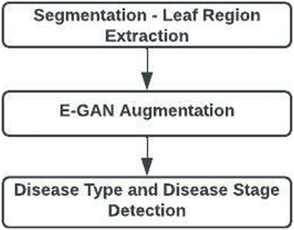
Figure 1: Overall architecture of proposed work

Segmentation: For high-throughput plant phenotypic data processing and quantitative studies of complex features, leaf segmentation is by far the most direct and efficient method. To separate the regions with leaves from those without, the circular Hough transform is used with the graph-based leaf extraction approach.

Augmentation: A method for artificially expanding the data collection is image augmentation. This is useful when we are provided a data set with a small number of data samples. When we train a Deep Learning model on a small number of data samples, the model tends to over-fit. With the E-GAN approach, illness traits are extracted from the photos and combined with healthy images.

Disease Detection: CNN plays a major role in recognizing plant leaf diseases. The capsule neural network is used to identify the disease types and their stages. It finds the basic features which are formed as capsules. The disease types and disease stages are identified by processing basic features of spatial and frequency information.

2  Methods and Material

2.1 Segmentation

With the least amount of human intervention possible, the segmentation model suggested in this research can extract leaves from the provided plant photos. Fig. 2 displays the suggested technique. The process involves three steps: leaf extraction, image improvement, and leaf counting. The statistical approach for removing the lighting effect, the graphing model for extracting the leaves, as well as the CHT for counting the leaves have all been used in the suggested technique.

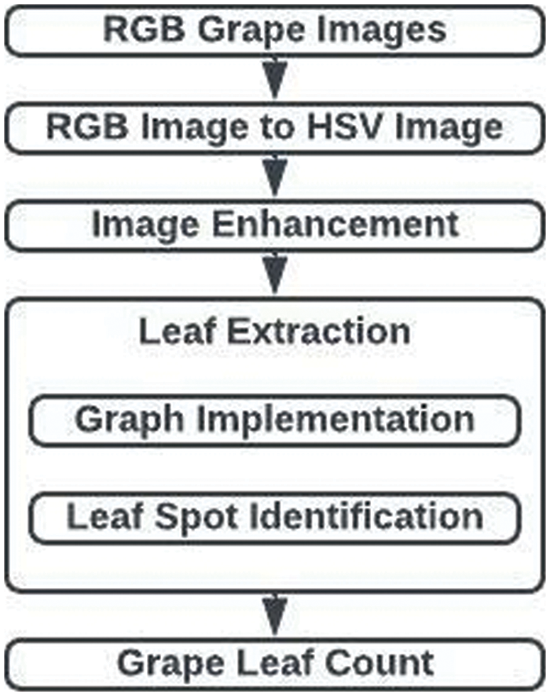
Figure 2: Leaf region segmentation

2.1.1 Image Enhancement

The probability distribution value of an image may be used to analytically compute the statistical features of a picture in statistical research of contrast enhancement [30]. The proposed research assumes that the brightness distribution follows the Weibull distribution. The probability density function (pdf) of the Weibull distribution is provided by recognizing an image [31]. In the suggested work, the plant’s red-green-blue (RGB) picture is first transformed into a hue-saturation-value (HSV) image. Since the V plane of an HSV picture correlates to the luminance of the image, image enhancement is done there. Let’s say that the V-plane pixels are represented as {x11, x12,…xmn}, where m and n are the plane’s corresponding row and column numbers. Calculations are made to determine the probability distribution of the skewness (Sk) and the V plane (provided in Eq. (1)).

Sk=(E(xij−μ)3)/σ3 (1)

where xij is the (i, j) th pixel value in the original HSV picture’s V plane, E stands for the expected value, μ stands for the mean value, and σ stands for the standard deviation. The V plane’s augmentation is necessary to eliminate the lighting impact whether the V plane’s skewness (Sk) is positive or negative.

2.1.2 Leaf Extraction

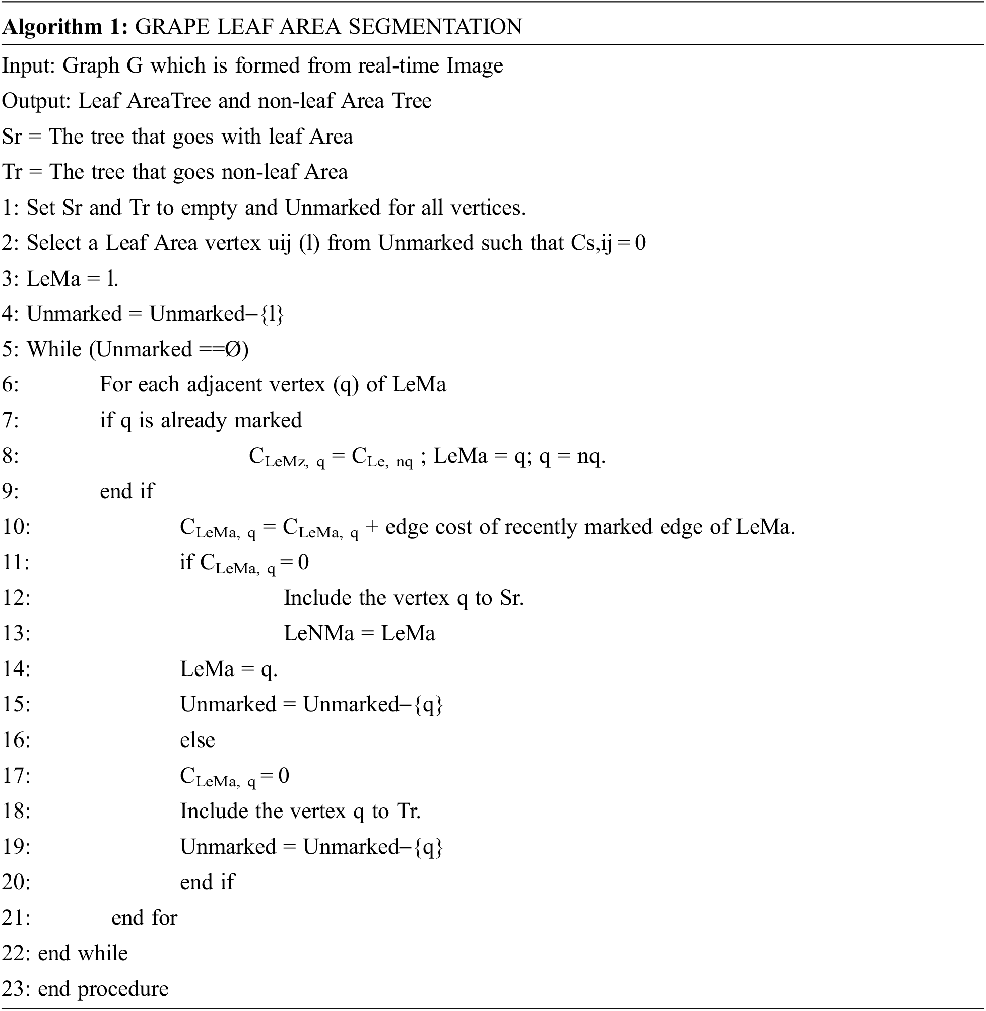
The suggested technique segments the leaf area using a graph-based algorithm, which improves segmentation accuracy while preserving resilience to reflection and shades. The efficiency of the suggested leaf separation technique is determined by the rows and columns count in the picture, The leaf extraction procedure is divided into two stages. They are (a) building a graph and (b) identifying leaf regions.

(a) Graph Construction

The graph is built using an improved HSV picture, which is segmented into leaf regions. The graph Gr = (U, E) for an improved HSV picture is created as seen in Fig. 3. The first point of the improved HSV picture serves as the starting point for the graph formation process, while the final pixel serves as the finishing point. The edges in a graph may be divided into two categories: (i) edges connecting two adjacent pixels, and (ii) edges connecting a pixel with a source or terminal. The edge cost determines how the HSV image’s pixels are related to one another. An edge cost is given to each edge in the graph.

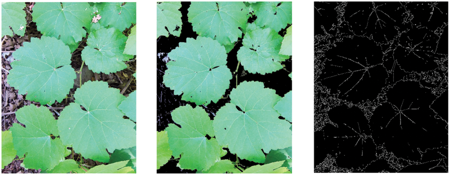
Figure 3: Graph construction from the original image

The edge costs Cs,ij (between the pixel uij and the source node sg), Cij,ij+1 (between the two adjacent pixels uij+1 and uij), and Cij,t (between terminal node tg and the pixel uij) may be computed to partition the leaf area.:

Cs,ij={0,ifPijistrue1,otherwise (2)

The edges cost between the pixel (uij) and the source node (sg) is Cs,ij. The association among pixels is predicted using the Pij. If there is indeed a connection between the pixels, the Pij is made to true; otherwise, it is set to false.

Cij,ij+1={0,ifPij∧Pij+11,otherwise (3)

where Pij and Pij+1 are the edge cost expectation parameters for the adjacent pixels uij and uij+1, respectively, and Cij,ij+1 is the edge cost among the pixels uij and uij+1.

Cij,t={1,ifPijistrue0,otherwise (4)

where Cij,t denotes the edge cost among the terminal node (tg) and the pixel (uij). The graph for fragmenting the leaf area of the provided plant picture is built using Eq. (2) through (4).

(b) Leaf Region Identification

The suggested graph-based approach (Algorithm 1) is used to separate the leaf area from the background once a graph for the source plant picture has been built as shown in Fig. 3. The route discovered in the proposed approach to divide the leaf area starts at the source vertex. Two distinct search trees source (Sr) and terminal (Tr), both from the terminal vertex and the source vertex, is formed to determine the route. When there are surrounding edges linking the internal vertices apart from the source and terminal with equal weights, these trees are utilized again to partition the leaf area and non-leaf region to prevent discovering the route beginning from the source vertex or terminal vertex. The search trees Sr and Tr are empty at the beginning and all of the vertices in a graph are assumed to be unmarked. The unmarked vertices are chosen as the starting vertex for the search tree Sr. This chosen vertex is now a “leaf margin” vertex for the Sr tree. Next, the “leaf margin” node’s neighbor edges are investigated; if the edge cost is zero, the specific neighbor vertex is added to the Sr tree. Otherwise, it is added to the Tr tree, and it is then deemed to be a marked vertex. If a new vertex is added to the Sr, the leaf margin vertex will change to a leaf non-margin vertex and the newly added vertex will take the place of the leaf margin vertex. The edge cost of the recently marked edge of the “leaf margin” vertex is combined with the edge cost of the unseen adjacent edges of the “leaf margin” vertex, and if the total edge cost is zero, makes the unmarked adjacent vertices as “leaf margin” vertices of the Sr. If not, the Tr is expanded with the relevant unmarked adjacent vertices to “leaf margin” vertices. The leaf margin vertex changes to the “leaf non-margin” vertex after all of its adjacents have been searched, and the newly inserted vertex changes to the “leaf margin” vertex if at least one adjacent vertex is inserted into the search tree Sr. The non-leaf region border and the interior non-leaf region, respectively, are represented by the non-leaf region vertices in the search tree Tr, which contains two kinds of vertices similar to the Sr: “non-leaf margin” vertices and “non-leaf non-margin” vertices. When a leaf margin vertex in the search tree Sr discovers a neighbor vertex that is a part of the search tree Tr, a path is discovered. The leaf area and the non-leaf area are represented by the vertices in the search trees Sr and Tr, respectively. When each vertex in the graph is added to the Sr_tree or Tr_tree, the algorithm converges. The graph-based leaf area separation is described by algorithm 1.

In the above algorithm, where uij denotes intermediate vertex, LeMa denotes Leaf_margin vertex, LeNMa denotes Leaf non-margin vertex, Cs,ij denotes edge cost/weight between uij (l) and the source vertex, CLeMa,q denotes edge cost/weight between LeMa and the neighbor vertex (q) of uij, nq denotes non marked nearest Leaf area vertex and CLe,nq denotes edge cost/weight among nq and its unmarked neighbor vertex.

2.1.3 Leaf Count

Circular Hough Transform [32] is used to count spherical grape leaves. The leaf numbering phase gets the extracted leaf region. Circular Hough Transform is employed across the leaf area. Each leaf is counted by its circular area. The circle shows the plant’s leaf area.

2.2 Augmentation

E-GAN, a local grape leaf feature-based data augmentation approach, was suggested in this work. Object identification, picture segmentation, and generative adversarial networks were all combined in the new technique. Because the leaf backdrop is a healthy picture, CNN was utilized to identify and segment grape leaf disease features. The suggested E-GAN may be separated into two steps, as indicated in Figs. 4 and 5. The leaf disease feature localization and segmentation then data augmentation.

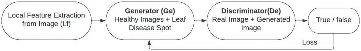
Figure 4: Flowchart of E-GAN

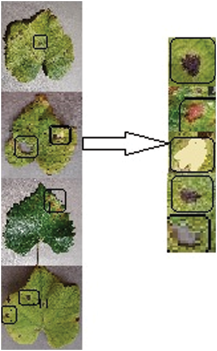
Figure 5: Disease area location and segmentation

2.2.1 Leaf Disease Area Location and Segmentation

The Convolution neural network was used to locate and segment grape leaf spot areas in this investigation. Local entity characteristics such as tiny circle patches, large circle patches, and yellow-colored patches are discovered by the CNN layer. As input into generators, the suggested E-GAN attempted to partition the similar size of major disease area bounding box.

2.2.2 Local Features Data Augmentation

The E-GAN emphasizes sickness spot image information and minimizes background interference. The intended E-GAN is described in full below.

1.   As the unmarked image parts L, choose the partitioned sub-images whose backdrop does not include leaf boundary background data. Assume that L = {l1, l2, l3… ln }is a dataset that contains the leaf disease object classifications

Lf=(Fi−Hs) (5)

where Lf denotes the leaf disease portion of the picture, Fi denotes the whole image, and Hs denotes the image’s healthy parts.

2.   Stage 2 is the augmentation stage. The suggested technique now mixes the grape leaf disease spot with the healthy photos and uses the generator to create new images (Ge). The discriminator (De) then determines if the freshly produced pictures are legitimate or fraudulent. The generator value and discriminator value are modified using the error or loss function.

Ge=(Lf−H) (6)

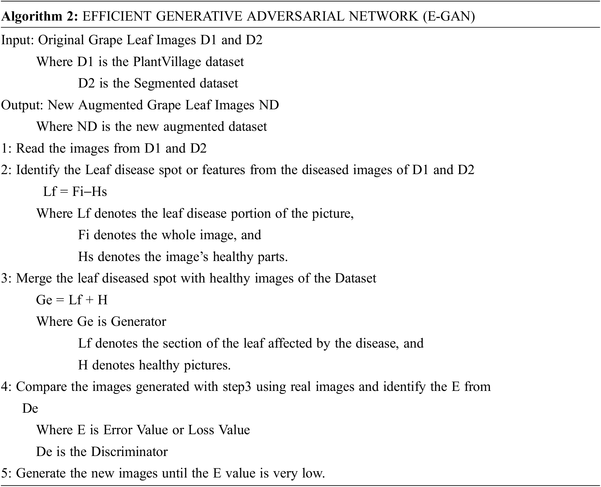
The E-GAN algorithm started with reading the images from the public dataset. The local features are extracted from the images and these features are passed to the generator with healthy images. Then the generated images are compared with the original images using a discriminator. The discriminator gives the loss value or error value which is used to adjust the generator function. GANs, as we know, can get the distributions of actual and produced pictures, and their purpose is to make the two distributions as similar as feasible.

2.3 Plant Leaf Disease and Disease Stage Detection

Capsule Networks were introduced by Hinton and his colleagues as an alternative to CNN. Capsules are non-comparable networks of neurons that accept and output vectors rather than scalar values like CNNs. This feature determines a capsule’s ability to learn about a picture’s properties, as well as its distortions and inspecting circumstances. Each capsule in a network of capsules is constructed from a network of cells, each of whose outputs represents a unique surface with a related attribute. This has the benefit of allowing us to recognize the entire thing by first recognizing its components.

The capsule network is defined using three layers: an input layer, a hidden layer, and an output layer. Pre-processing procedures are found in the input layer. To save time, the picture is downsized to 256 by 256 pixels. A convolution layer with a kernel size of 9 is referred to as a hidden layer. The filter’s dot product and portions of the input pictures are used in the convolution layer. Capsules are made using convolution and the primary caps layer. Capsules are made up of layers of neural tissue that are layered on top of each other. The probability distribution is determined by the neural network’s last layer, which consists of a fully connected layer followed by softmax activation. In the linked layer, every neuron in one layer is coupled to every neuron in another one.

The softmax equation is as follows:

softmax=SF(x)i=eyi∑j=1neyi (7)

where xi represents the i-th item of the vector.

Finally, categorical cross-entropy assesses the prediction loss of the deep learning model.

loss(L,e)=−∑yp(y)log⁡(e(y)) (8)

where L is a true probability distribution.

The recommended design is unique for datasets related to grape plants. Increased parameters may be utilized to further extend the model, allowing us to address issues with grape plants. The recommended architecture can be regarded as shown in Fig. 6. The proposed design includes an encoder and decoder. The encoder’s first three layers turn the input image into a vector. The initial layer of the encoder’s convolutional neural network collects tiny circle patches, big circle patches, and yellow patches. The secondary capsule searches for detailed patterns among the essential features. It may sense spatial relationships between strokes. The grape leaf photo dataset in PrimaryCaps Network has 32 capsules. The third layer is capsule processing, and its number varies. After these phases, the encoder generates a 4-dimensional vector. The decoder has two layers. It utilizes the 4-dimensional vector to reconstruct the picture from scratch and match it with the illness type and stages. The network’s capacity to make expert-based predictions makes it more robust.

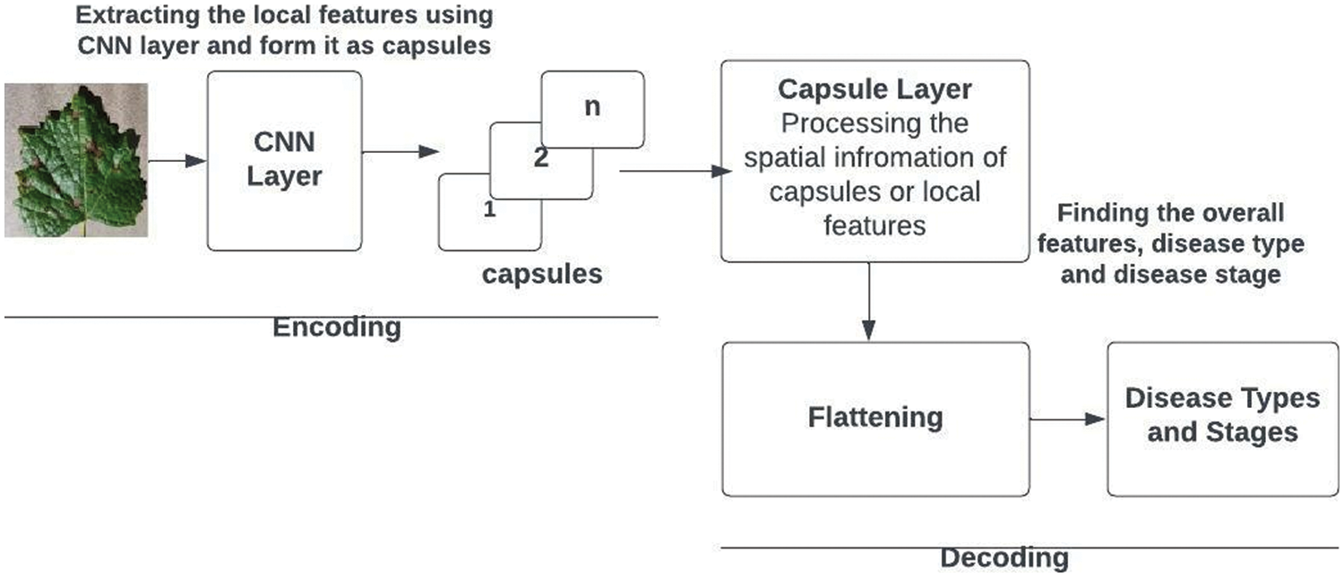
Figure 6: Capsule network architecture for grape plant leaf disease and stage detection

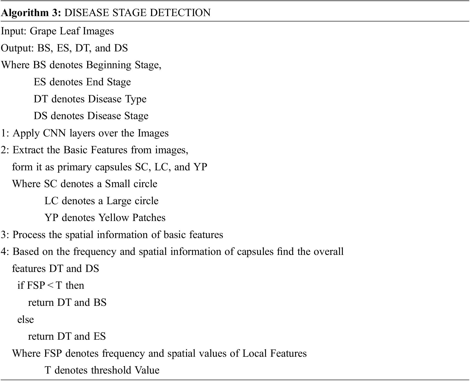
Algorithm 3 shows how the disease types and stages are identified. Capsules are neuronal groupings that store spatial and frequency information as well as the likelihood of an item being there. In a capsule network, for each entity in a picture, there is a capsule that provides the possibility that the entity exists as well as the spatial parameters of that entity. The CNN layer finds local entity features such as small circle patches, Big circle patches, and yellow-colored patches. The capsule layer is used to collect the overall features such as “disease type” and “disease stage,” using the low-level features frequency and spatial information.

Cap=CNN(I):f(SC,LC,YP) (9)

FSP=Fr(Cap)+Sp(Cap) (10)

Eq. (9) represents the capsules that are formed by extracted features like small circles (SC), large circles (LC), and yellow patches. In Eq. (10), The frequency and spatial information of each capsule or basic features are determined by combining the frequency of the capsule and spatial details of the capsule.

3  Dataset and Experimental Design

There are two kinds of datasets used for this proposed work. The first datasets, which are used for the proposed segmentation work captured using a Canon SD1000 camera in the Theni district, Tamilnadu, India. Images for the dataset are taken once every six hours throughout the day for three weeks. It is made up of 112 (500,530 pixels) photos with dynamic backgrounds. The segmented pictures are created from real-time photos as seen in Fig. 7.

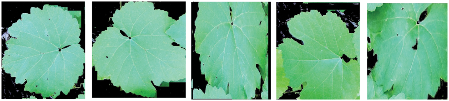
Figure 7: Segmented grape leaf images

The segmented images of 500 from real-time images and the second kind of dataset known as PlantVillage grape datasets are used for augmentation and disease detection. This augmentation and disease detection required a high-performance computing platform for training and testing. 1000 healthy leaf pictures and 1500 grape leaf disease images were sorted into three categories in the PlantVillage dataset and 500 real-time images which are segmented using graph-based segmentation were used as the dataset. The three kinds of grape leaf disease images are black measles, black rot, and late blight. The grape leaf disease spots are identified from the three disease categories of the dataset and segmented grape leaves. Then synthesized diseased grape leaf pictures dataset was created by embedding disease spots with healthy images with the E-GAN method. Black measles is caused by a variety of fungi. “Striping” is the most common symptom of black measles. A fungus causes black rot in grapes. The black rot disease signs appear on infected leaves, tiny brown round scratches appear on occasion. When the weather is hot and humid, grape leaves are susceptible to leaf blight. This disease may create huge lesions on fresh grape leaves with black or dark red patches, resulting in catastrophic loss. Fig. 8 shows four typical pictures from the PlantVillage [33] grape data set, with the variations between the four types of pictures readily visible.

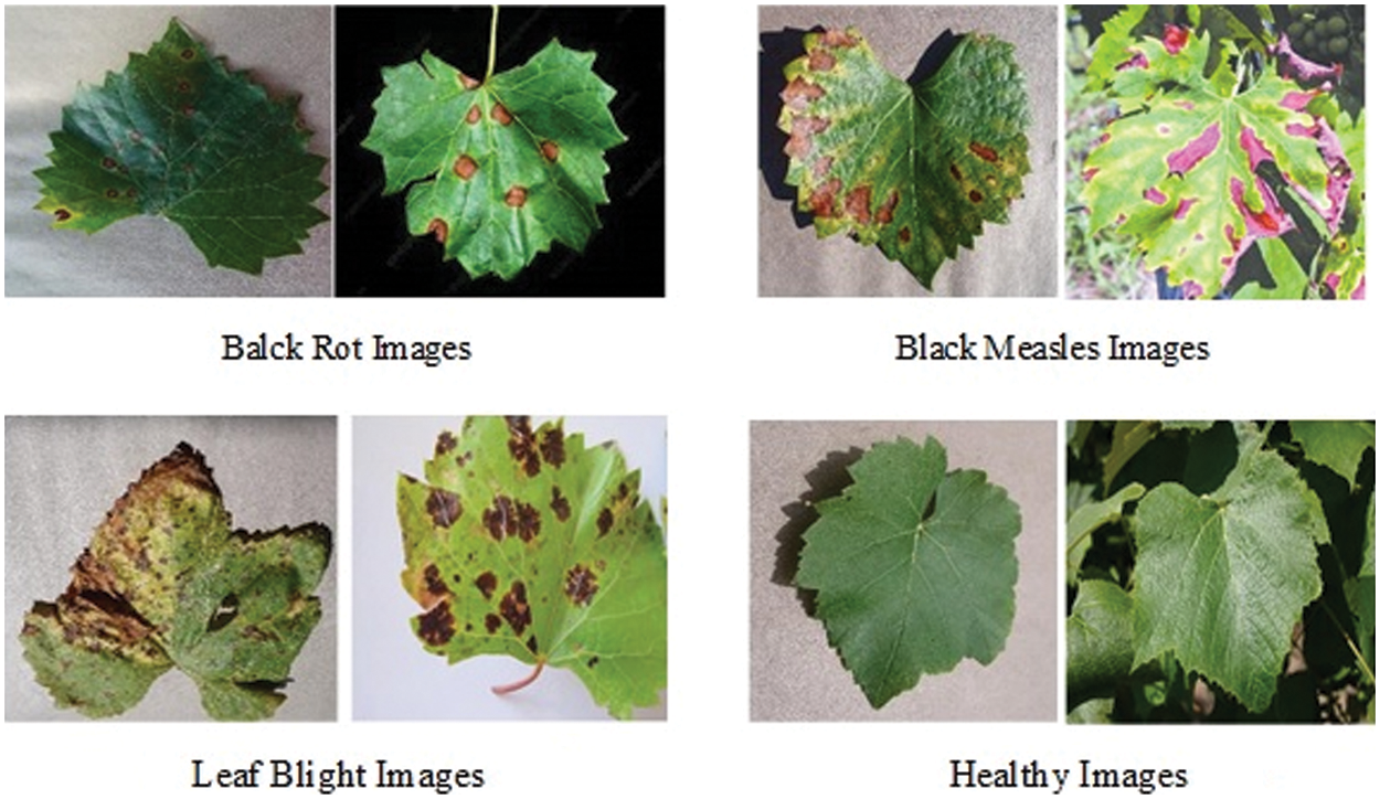
Figure 8: Four types of grape leaf images

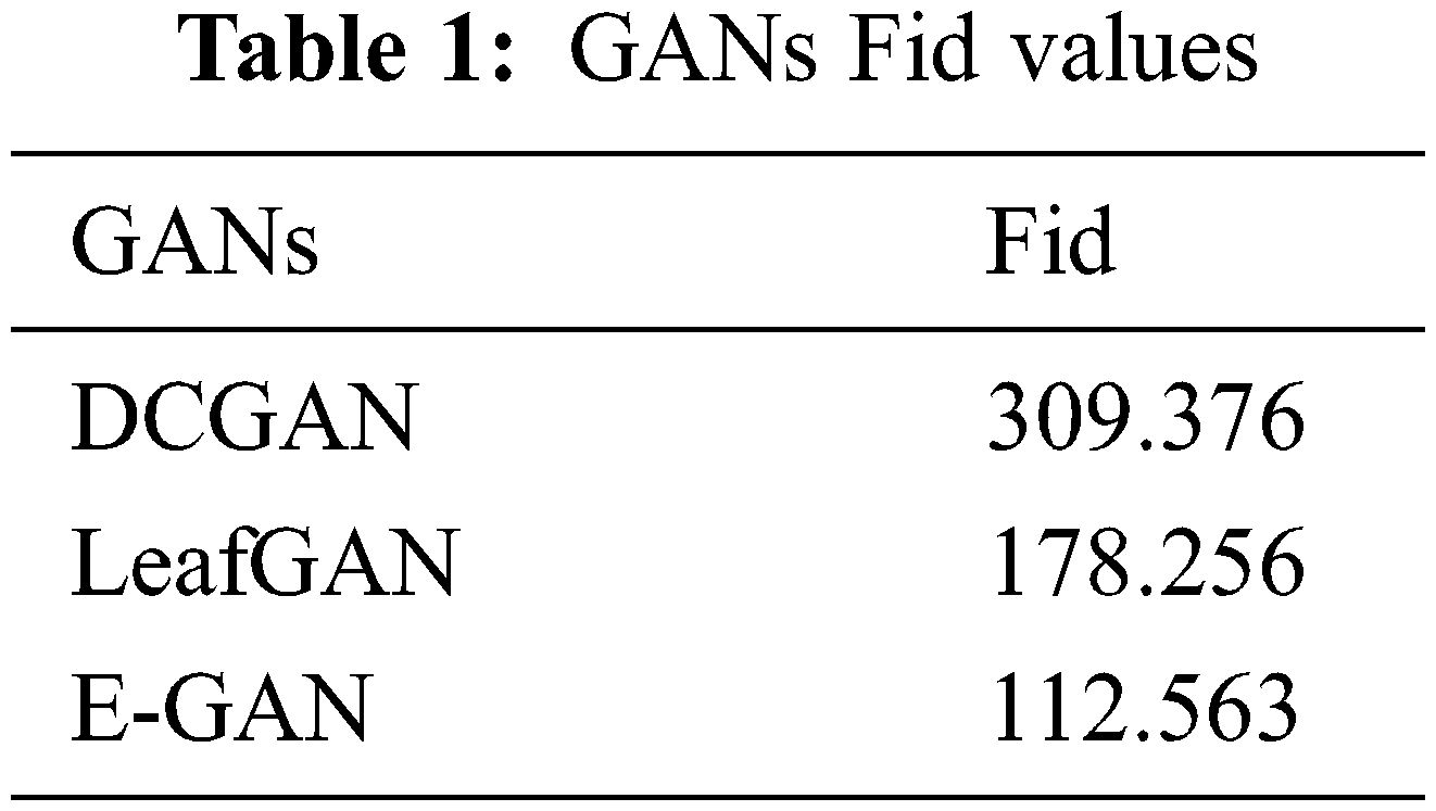
Frechet Inception Distance (Fid) [34] was used to evaluate GAN designs. We produced 1000 real-time segmented photos and 4000 PlantVillage images for this investigation. Table 1 displays GAN Fid. Table 1 shows that the suggested approach had the lowest score, suggesting it can produce superior photos.

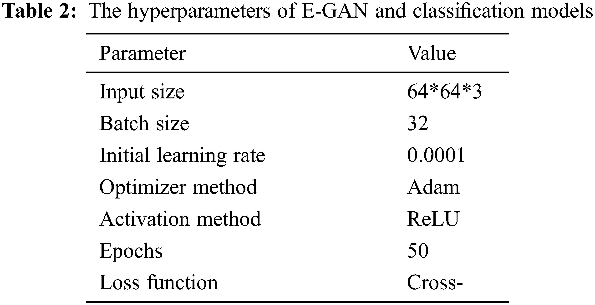
The classification models used in this study were state-of-the-art, including visual geometry group −16 (VGG-16), AlexNet [35], and Xception [36]. Pre-trained models are networks that have been trained on large datasets, usually images. We may use the pre-trained network as-is or transfer learning to customize it. We may import a pre-trained version of these networks from the PlantVillage database. These networks can classify photographs into 1000 categories, including sickness. Every one of these models conducted data augmentation on the distinct training data sets: original images without data augmentation, DCGAN data augmentation, and recently published data improvement approaches such as LeafGAN [37] and E-GAN data augmentation. Table 2 shows E-GAN and classification model hyperparameters.

The loss value is one of the most significant methods for determining the difference between the network output and the desired output. It was shown that the cross-entropy loss function and the softmax activation function were both more convenient ways of dealing with the multi-classification issue in the loss layer and output layer, respectively.

4  Experimental Results and Discussions

4.1 E-GAN

There were four different types of grape leaf graphics. 80 percent of the training dataset and 20% of the test set were made up of three types of grape leaf pictures with sick, real-time segmented grape leaf images and one kind of good grape leaf. The categorization findings from the testing set are given in Fig. 9 after 50 epochs employing VGG16, AlexNet50, and Xception with the original dataset. The four types of grape leaf pictures are shown on the horizontal plane from 1 to 4. The data set was then expanded using DCGAN and LeafGAN. The expanded data set includes 1000 images of each grape leaf, with 80% acting as training data and 20% as test data. The classifying results for the testing dataset are displayed in Figs. 10 and 11 after 50 epochs employing VGG16, AlexNet, and Xception with DCGAN and LeafGAN. The data set was expanded using E-GAN to the very same number of pictures and train modes as before. Fig. 12 shows the categorization findings from the test set.

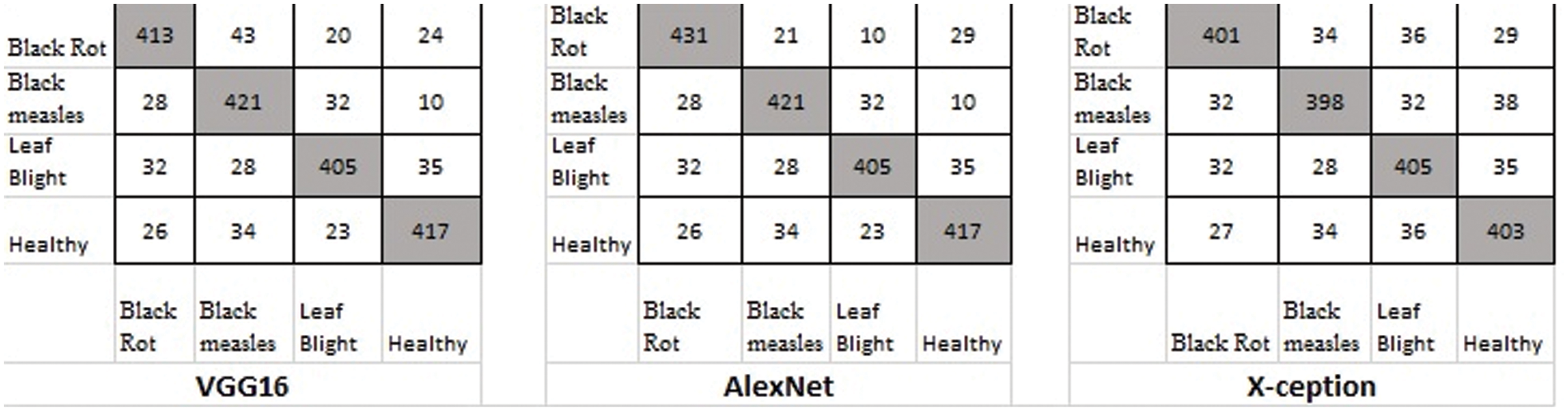
Figure 9: Classification result based on the original dataset

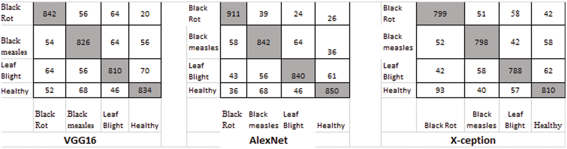
Figure 10: Classification result using DCGAN

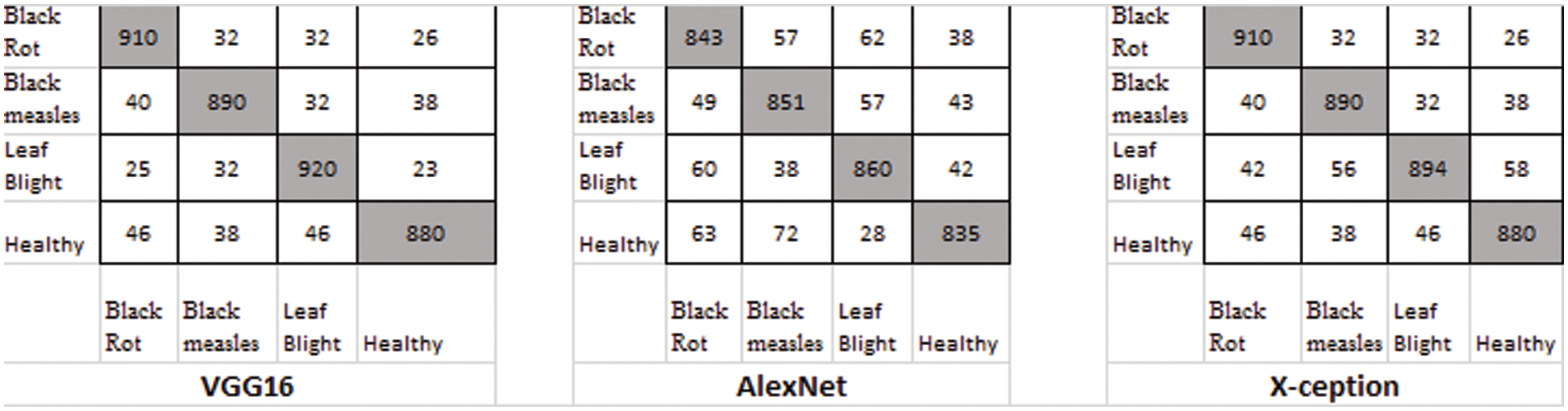
Figure 11: Classification result using LeafGAN

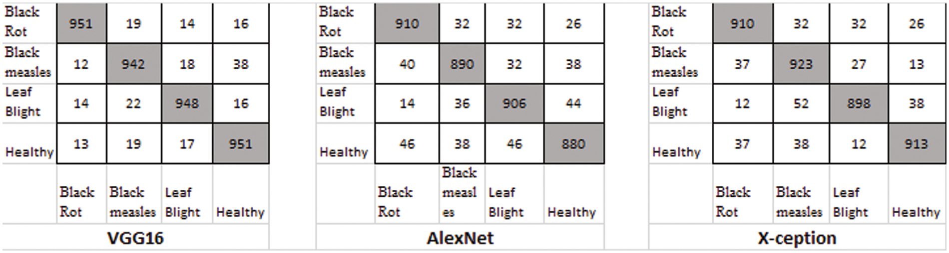
Figure 12: Classification result using the E-GAN method

Table 3 shows the average results of three GANs for data expansion and no data augmentation as training data for the three standard deep learning models, as well as the results of the three state-of-the-art deep learning models. Most of these deep learning models, except for X-ception, are unable to yield adequate results when no data expansion is performed, according to this finding. The fundamental reason behind this is that various models, such as AlexNet, VGG-16, and X-ception, offended from overfitting due to insufficient training data. As a result, they were unable to achieve the capability of feature extraction and consequently performed poorly.

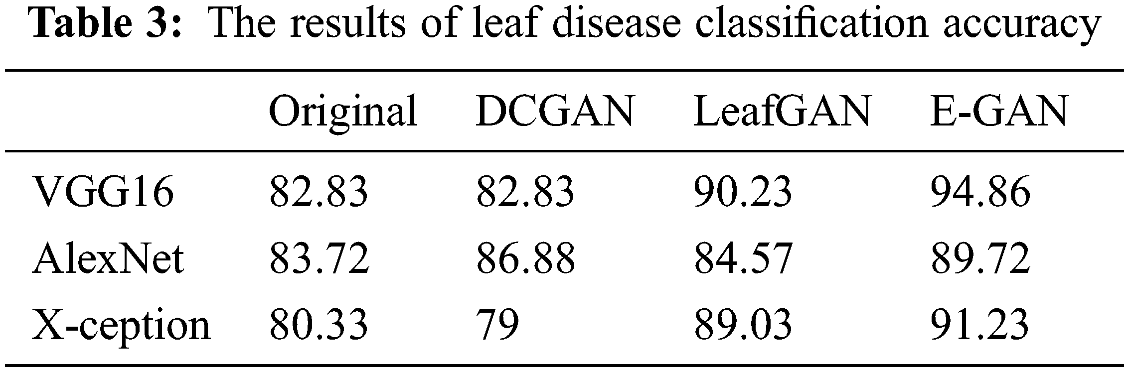
When GANs employed the data augmentation techniques, the accuracy of all three Generative adversarial data augmentation methods was greater than the accurateness of none of the data expansion methods when none of the data augmentation methods was used. However, other models, such as X-ception, experienced worse performance as a result of data expansion using DCGAN, the primary explanation for this approach was that the pictures created by DCGAN were of poor quality. We were unable to adjust to the models we were given. On top of all that, the suggested method had reached reasonable effects on the above-mentioned models, which demonstrated that the suggested method possessed a more solid data augmentation capability than other GANs in terms of making disease features more observable while simultaneously reducing background errors to a significant degree. In comparison to typical data expansion approaches, the suggested approach combined local disease features with a healthy image synthesis algorithm, resulting in more successful identification, particularly in sparse distributions of tiny targets. The produced local disease area pictures were included in the original healthy images for training in the grape leaf disease spot identification experiment, which improved the generalization capacity of the classification models and improved the accuracy and robustness of the prediction. In comparison to the previous GANs stated above, the suggested E-GAN was better in spot localization and picture segmentation, and the hierarchical mask generation improved disease feature representation. However, the suggested approach has the drawback of being limited to the instance of leaf spots; when the plant leaf syndrome is not visible as spots, the method’s effectiveness is substantially diminished. We will continue to research other phonemics in plant disease detection in the future.

4.2 CapsuleNet Performance

It was intended to employ grape leaves in conjunction with the capsule network for categorization, and it was successful. The first three investigations in Table 4 are all based on the CNN algorithm. As can be seen, this capsule neural network model (CapsNet) works well. When comparing calculation times, it is clear that CNN-centered algorithms are more efficient. When examining the table, the capsule neural network approach produced a greater accuracy rate than other methods with disease stages information. It calculates the disease stage just by comparing the threshold value with the frequency of features. In comparison to other approaches, it takes longer to infer. The reason behind this is that the suggested method’s multilevel features enhance the model’s complexity. It also needs to process the spatial information of basic features. This is where the suggested model falls short, and it will need to be modified in the forthcoming research.

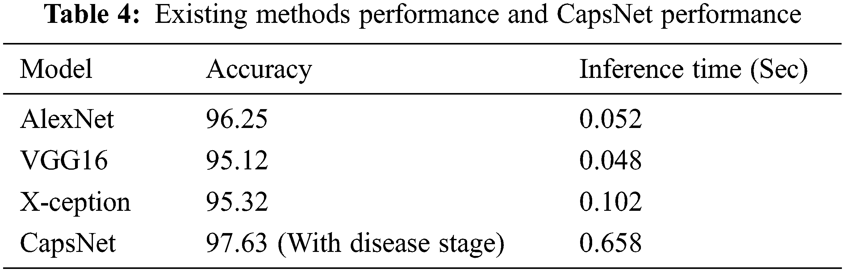
The accurateness of this CapsNet model for grape plant leaf infection is identified as 97.63% based on the confusion matrix which is given in Fig. 14. The accomplishment of the proposed approach for each class is depicted in the confusion matrix in Fig. 14. This allows for a visual examination of the classifier’s performance. The real class is specified by the columns, whereas the output class is determined by the rows. Non-diagonal cells represent erroneously classed observations, whereas diagonal cells represent mistakenly classified observations. The results were computed and reported as a percentage using the indicated technique on the test data. When looking at Fig. 13, it is clear that all classes are categorized with great accuracy. This demonstrates that the suggested approach has a high degree of discrimination. Only second-grade black measles has a worse classification accuracy rate. The minimal number of samples in this class is assumed to be the cause of this problem. A comparative study and research employing the capsule neural network model for grape plant disease identification are presented in Table 4. The stages of diseases are also identified based on the frequency of the features. All approaches were applied to the data set utilized in this study for a fair comparison. The trials were carried out on the same computer, which was programmed in Python.

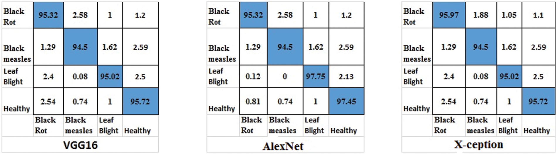
Figure 13: Confusion matrices for ResNet18, VGG16 and GoogleNet

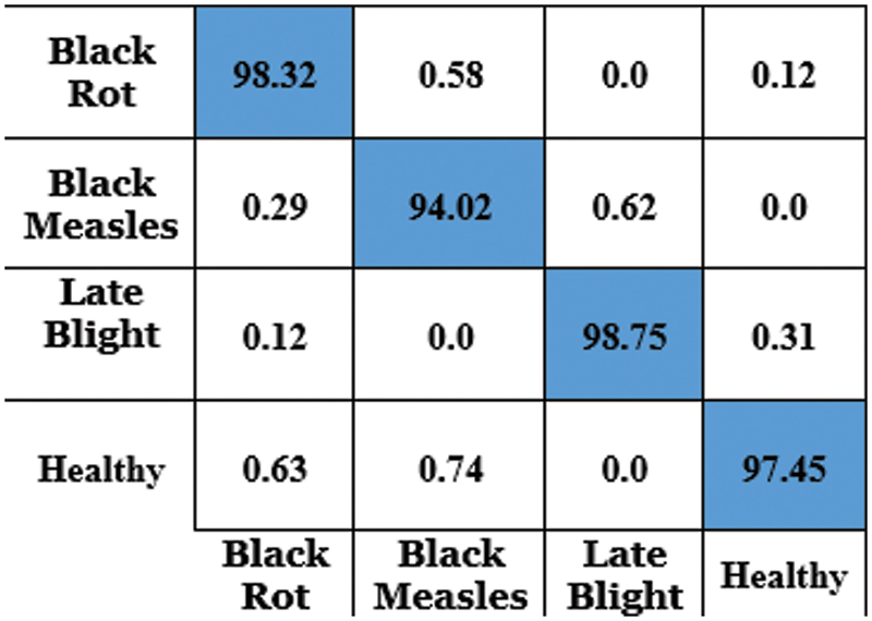
Figure 14: Confusion matrix for grape leaf disease detection using CapsNet

The capsule neural network model initially identifies the local features from the images. Then it processes the spatial information like frequency and direction of the extracted features. And based on the frequency of local features which is mentioned in the disease stage identification algorithm, It returns the output either as early-stage disease or end-stage disease.

The confusion matrix in Fig. 12 demonstrates the classification accuracy of the E-GAN approach using four different forms of plant leaf diseases: black rot, black measles, late blight, and healthy leaves. When combined with E-GAN, classic classification models such as Alexnet, VGG16, and X-ception provide superior results. The capsule neural network that incorporates E-GAN produces results that are superior to those of classic models. Additionally, it determines the stage of the illness that affects the grape leaves. Using the local features threshold count condition, the Routh-Hurwitz stability criteria [38] may be used to determine whether the leaves are well-infected. If the number of local characteristics that were retrieved using the capsule model was larger than three, then the illness was judged to be at its end-stage, as shown in Fig. 15. If the number of extracted characteristics is fewer than or equal to 3, this condition will be classified as an early stage of the illness.

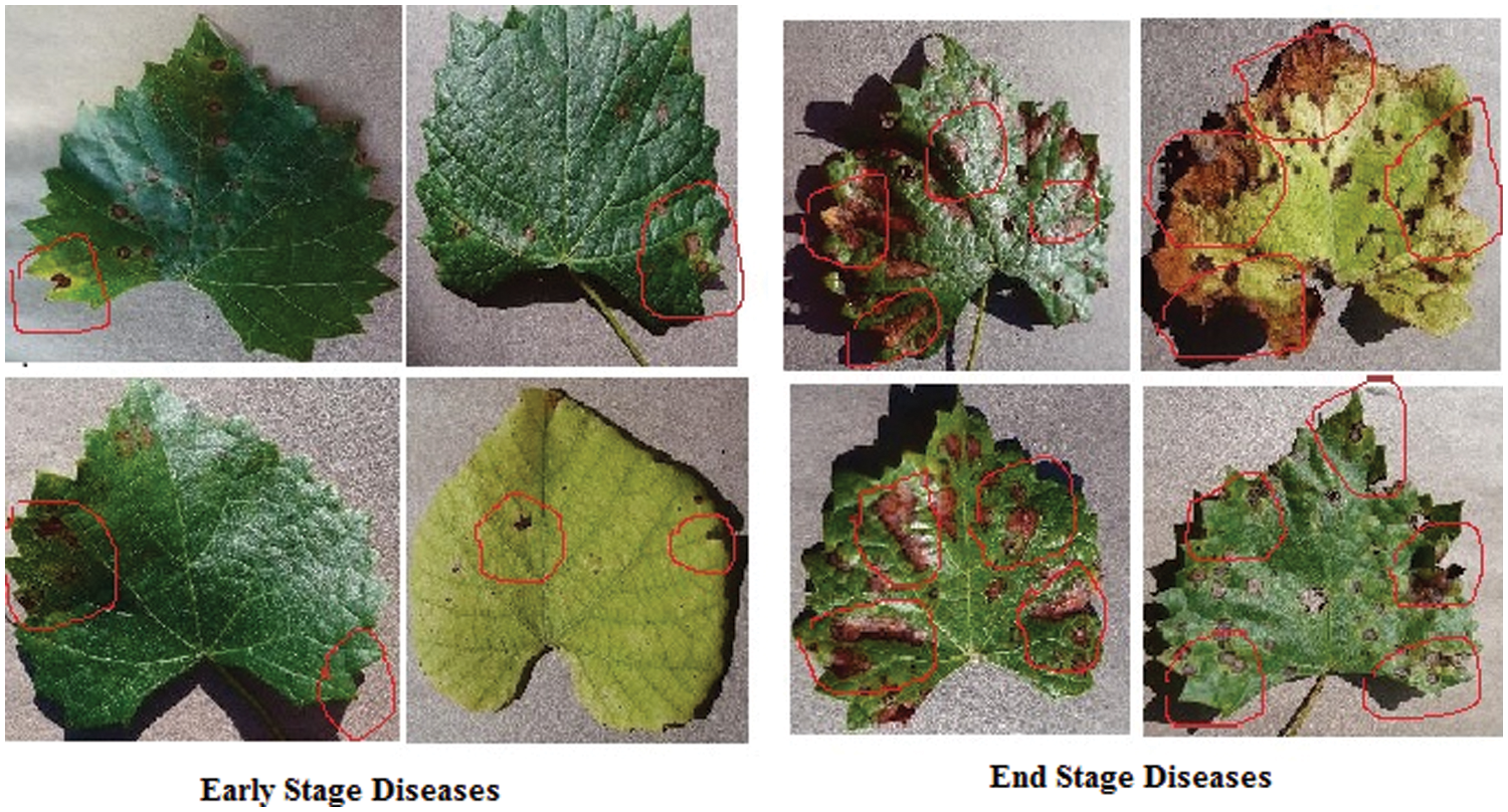
Figure 15: Early and end stages of diseases

5  Conclusions

A new hybrid method for grape leaf disease detection and disease stage detection using segmentation, augmentation, and a capsule neural network is proposed. The experimentations are carried out and evaluated for grape leaf disease detection and disease stage detection using real-time images and the PlantVillage dataset. The proposed method is compared with various existing CNN models. It achieves an accuracy of 97.63% which is higher than the existing model. In the future, this hybrid model will be able to be further fine-tuned to discover the causes for, and solutions to, the identification of plant diseases.

Funding Statement: The authors received no specific funding for this study.

Conflicts of Interest: The authors declare that they have no conflicts of interest to report regarding the present study.

References

 1.  M. Minervini, A. Fischbach, H. Scharr and S. A. Tsaftaris, “Finelygrained annotated datasets for image-based plant phenotyping,” Pattern Recogn Letters, vol. 81, no. 1, pp. 80–89, 2016. [Google Scholar]

 2.  S. Mahajan and A. K. Pandi, “Image segmentation and optimization techniques: A short overview,” Medicon Engineering Themes, vol. 2, no. 2, pp. 47–49, 2022. [Google Scholar]

 3.  D. Li, G. Shi, W. Kong, S. Wang and Y. Chen, “A leaf segmentation and phenotypic feature extraction framework for multiview stereo plant point clouds,” IEEE Journal of Selected Topics in Applied Earth Observations and Remote Sensing, vol. 13, pp. 2321–2336, 2020. [Google Scholar]

 4.  Q. Yunli, C. Gao and Y. K. Li, “Advances in genetic studies of black point disease in wheat,” Journal of Plant Diseases and Protection Springer, vol. 128, no. 4, pp. 887–895, 2021. [Google Scholar]

 5.  M. G. Brochier, A. Vacavant, G. Cerutti, C. Kurti, J. We et al., “Tree leaves extraction in natural images: Comparative study of preprocessing tools and segmentation methods,” IEEE Transaction Image Process, vol. 24, no. 5, pp. 1549–60, 2015. [Google Scholar]

 6.  N. V. de Almeida, E. B. Rivas and J. C. Cardoso, “Somatic embryogenesis from flower tepals of hippeastrum aiming regeneration of virus-free plants,” Plant Science Elsevier, vol. 317, no. 111191, 2022. [Google Scholar]

 7.  L. Zhang, Q. Nan, S. Bian, T. Liu and Z. Xu, “Real-time segmentation method of billet infrared image based on multi-scale feature fusion,” Scientific Reports, vol. 12, no. 1, pp. 6879–6884, 2022. [Google Scholar]

 8.  J. Arunpandian, V. Dhilipkumar, O. Geman, M. Hnatiuc, M. Arif et al., “Plant disease detection using deep convolutional neural network,” MDPI Applied Science, vol. 12, no. 1, pp. 14–19, 2022. [Google Scholar]

 9.  S. Mahajan, L. Abualigah, A. K. Pandit and M. Altalhi, “Hybrid aquila optimizer with arithmetic optimization algorithm for global optimization tasks,” Soft Computing, vol. 26, no. 237, pp. 4863–4881, 2022. [Google Scholar]

10. J. Ma, K. Du, F. Zheng, L. Zhang and Z. Sun, “Disease recognition system for greenhouse cucumbers based on deep convolutional neural network,” Nongye Gongcheng Xuebao/Transactions of the Chinese Society of Agricultural Engineering, vol. 34, no. 12, pp. 186–192, 2018. [Google Scholar]

11. S. Mahajan and A. K. Pandit, “Hybrid method to supervise feature selection using signal processing and complex algebra techniques,” Multimedia Tools and Applications, vol. 70, no. 1, pp. 1–22, 2021. [Google Scholar]

12. S. Mahajan, L. Abualigah and A. K. Pandit, “Hybrid arithmetic optimization algorithm with hunger game search for global optimization,” Multimedia Tools and Applications, vol. 81, no. 7, pp. 28755–28778, 2022. [Google Scholar]

13. M. Faye, C. Bingcai and K. A. Sada, “Plant disease detection with deep learning and feature extraction using plant village,” Journal of Computer and Communications, vol. 8, no. 6, pp. 10–22. 2020. [Google Scholar]

14. J. Sun, W. Tan, H. Mao, X. Wu, Y. Chen et al., “Recognition of multiple plant leaf diseases based on improved convolutional neural network,” Transactions of the Chinese Society of Agricultural Engineering, vol. 33, no. 19, pp. 209–215, 2017. [Google Scholar]

15. A. Creswell, T. White, V. Dumoulin, K. Arulkumaran, B. Sengupta et al., “Generative adversarial networks: An overview,” IEEE Signal Processing Magazine, vol. 35, no. 1, pp. 53–65, 2017. [Google Scholar]

16. A. Sajeeda and B. M. Mainul Hossain, “Exploring generative adversarial networks and adversarial training,” International Journal of Cognitive Computing in Engineering, vol. 3, no. 1, pp. 78–89, 2022. [Google Scholar]

17. C. Yinkabanjo and O. A. Ugot, “A review of generative adversarial networks and its application in cybersecurity,” Artificial Intelligence Review, vol. 53, pp. 1721–1736, 2019. [Google Scholar]

18. Z. Zeng-Shun, G. Han-Xu, S. Qian, T. Sengh, D. O. Wu et al., “Latest development of the theory framework, derivative model and application of generative adversarial nets,” Journal of Chinese Computer Systems, vol. 39, no. 12, pp. 2602–2606, 2018. [Google Scholar]

19. Y. Du, W. Zhang, J. Wang and H. Wu, “DCGAN based data generation for process monitoring,” in Proc. Data Driven Control and Learning Systems Conf. (DDCLS), Beijing, China, pp. 410–415, 2019. [Google Scholar]

20. G. Qiang and J. Zhonghao, “Amplification of small sample library based on GAN equivalent model,” Electrical Measurement & Instrumentation, vol. 56, no. 6, pp. 76–81, 2019. [Google Scholar]

21. W. Xiaoqing, W. Xiangjun and N. Yubo, “Unsupervised domain adaptation for facial expression recognition using generative adversarial networks,” Computational Intelligence and Neuroscience, vol. 2018, pp. 1–10, 2018. [Google Scholar]

22. X. L. Tang, Y. M. Du, Y. W. Liu and J. X. Li, “Image recognition with conditional deep convolutional generative adversarial networks,” Acta Automatica Sinica, vol. 44, no. 5, pp. 855–864, 2018. [Google Scholar]

23. I. Su, X. Xu, Q. Lu and W. Zhang, “General image classification method based on semi-supervised generative adversarial networks,” High Technology Letters, vol. 25, no. 1, pp. 35–41, 2019. [Google Scholar]

24. D. Mahapatra, B. Bozorgtabar, R. Garnavi and S. Hewavitharanage, “Image super-resolution using generative adversarial networks and local saliency maps for retinal image analysis,” in Proc. Int. Conf. on Medical Image Computing & Computer-Assisted Intervention, Muscat, Oman, pp. 108–114, 2017. [Google Scholar]

25. Prabhat, Nishant and D. K. Vishwakarma, “Comparative analysis of deep convolutional generative adversarial network and conditional generative adversarial network using handwritten digits,” in Proc. Int. Conf. on Intelligent Computing and Control Systems, Dindukal, India, pp. 1072–1075, 2020. [Google Scholar]

26. T. A. Wagh, R. M. Samant, S. V. Gujarathi and S. B. Gaikwad, “Grapes leaf disease detection using a convolutional neural network,” International Journal of Computer Application, vol. 178, no. 20, pp. 7–11, 2019. [Google Scholar]

27. A. Raza, “Mathematical modeling of rotavirus disease through efficient methods,” Computers, Materials and Continua, vol. 72, no. 3, pp. 4727–4740, 2022. [Google Scholar]

28. B. Liu, Z. Ding, L. Tian, D. Hue and H. Wang, “Grape leaf disease identification using improved deep convolutional neural networks,” Frontiers in Plant Science, vol. 11, pp. 1082, 2020. [Google Scholar]

29. B. F. Oladejo and A. O. Olajide, “Automated classification of banana leaf diseases using an optimized capsule network model,” in Proc. Computer Science of Information Technology, Ibadan, Nigeria, pp. 119–130, 2020. [Google Scholar]

30. Z. Amini and H. Rabbani, “Statistical modeling of retinal optical coherence tomography,” IEEE Transaction in Medical Imaging, vol. 35, no. 6, pp. 1544–54, 2016. [Google Scholar]

31. K. T. Chang, “Analysis of the weibull distribution function,” Journal of Applied Mechanics, vol. 49, no. 2, pp. 450–461, 1982. [Google Scholar]

32. Q. Li and M. Wu, “An improved hough transform for circle detection using circular inscribed direct triangle,” in Proc. Int. Congress on Image and Signal Processing, BioMedical Engineering and Informatics (CISP-BMEI), Hangzhou, China, pp. 203–207, 2020. [Google Scholar]

33. D. P. Hughes and M. Salathe. “An open access repository of images on plant health to enable the development of mobile disease diagnostics,” arXiv 2015, [Online]. Available arXiv:1511.08060. [Google Scholar]

34. K. Kobayashi, K. J. Tsuji and M. Noto, “Evaluation of data augmentation for image-based plant-disease detection,” in Proc. IEEE Int. Conf. in System Man and Cybernetics, (SMC), Yokohama, Japan, pp. 2206–2211, 2018. [Google Scholar]

35. X. Zhang, J. Zou, K. He and J. Sun, “Accelerating very deep convolutional networks for classification and detection,” IEEE Transactions on Pattern Analysis and Machine Intelligence, vol. 38, no. 10, pp. 1943–1955, 2016. [Google Scholar]

36. V. M. Gutierrez, E. Carlos, G. Tejada, L. Garcia, S. Padilla et al., “Comparison of convolutional neural network architectures for classification of tomato plant diseases,” Applied Science, vol. 10, no. 4, pp. 1245–1253, 2020. [Google Scholar]

37. Q. H. Cap, H. Uga, S. Kagiwada and H. Iyatomi, “LeafGAN: An effective data augmentation method for practical plant disease diagnosis,” IEEE Transactions on Automation Science and Engineering, vol. 19, no. 2, pp. 1258–1267, 2022. [Google Scholar]

38. N. Ahmed, A. Raza, A. Akgül, Z. Iqbal, M. Rafiq et al., “New applications to Hepatitis C model,” AIMS Mathematics, vol. 7, no. 6, pp. 11362–11382, 2022. [Google Scholar]