A Lightweight Electronic Water Pump Shell Defect Detection Method Based on Improved YOLOv5s

1  Introduction

The electronic water pump is an important component of automotive engine cooling systems, and its performance has a direct effect on the operation of the engine. The main function of the electronic water pump is to drive the circulation of the coolant, absorb the excess heat generated by the engine and transfer it to the external air through a heat dissipation device to prevent the engine temperature from rising too high. Excessively high engine temperatures will prevent proper oil lubrication and result in increased wear; high temperatures beyond a certain threshold will lead to cylinder explosion or tile burning and other serious failures and ultimately lead to the engine being scrapped. The electronic water pump shell, as one of the main parts of the electronic water pump (as shown in Fig. 1), is prone to burrs, scratches, and other defects in the injection molding process, which dramatically affects the performance of the electronic water pump and can lead to insufficient cooling performance and therefore potentially dangerous problems. Real-time detection of the electronic water pump shell can effectively reduce the presence of unqualified products on the market and increase automobile safety. Therefore, we propose a network architecture for the real-time defect detection of the electronic water pump shell.

Figure 1: The electronic water pump shell

The defect detection of the electronic water pump shell is carried out manually. Because such defects are often small and the surface of the electronic water pump shell is complex, defects are often undetected because inspections are performed quickly and under extreme pressure. At the same time, there is uncertainty about the validity of the results generated by workers with different experience levels. Therefore, there is an urgent need for a method that can realize automatic inspection in real-time to change the status quo. The defects of electronic water pumps are often in the form of burrs and small surface scratches and do not relate to the materials and their quality, so image-based defect detection methods are the most direct, simple, and effective. Overall, replacing manual defect detection with an algorithm based on deep learning technology that uses a camera combined with a trained defect detection model to identify and distinguish objects or defects is both simple and practical and improves detection efficiency, thus freeing workers from having to perform tedious detection work.

Image classification was first tested using convolutional neural networks (CNN) [1]. Riaz et al. [2] proposed an innovative neural network that utilizes live camera occupancy detection and recognition for various types of sensors. In recent years, advances in computer algorithms have made them more competitive and abundant, and image classification algorithms have been rapidly developed. Many excellent classification models have been verified, such as VGG [3], GooLeNet [4], and ResNet [5]. Using a single network model is not sufficient for solving difficult problems and thus some researchers have contributed their research objects to improve the network model. Chen et al. [6] proposed a visual detection device for plastic gasket defects based on GoogLeNet InceptionV2 transmission learning to solve the problem of its surface defects being numerous and difficult to extract while classifying its features. Chakravarthi et al. [7] proposed a hybrid deep learning algorithm employing CNN-LSTM classification in combination with the ResNet152 model to identify human emotions. Lui et al. [8] proposed a new enhanced data-driven pedestrian tracking method for public buildings that use pedestrians’ trajectories to predict their destination. Riaz et al. [9] developed the MULTIMOORA method based on the q-ROF Einstein aggregation operator for MCDM to improve energy efficiency in low-income households at the national level in Pakistan. Xing et al. [10] proposed a fusion algorithm based on SURF and SWT for regional railcar positioning to locate the enhanced images produced by the improved single-scale Retinex algorithm. The results show that the accuracy of the method is 96.91% in complex cases.

Further achievements have been made using deep learning methods, such as the YOLO [11–13], RCNN [14–16], and SSD series [17,18], as well as R-FCN [19], in the detection of workpiece surface defects. Xing et al. [20] proposed an improved YOLOv3 rail wheel surface defect detection framework to solve the problem of conventional wheel defect detection techniques being unable to achieve automatic classification and accurate defect localization. Li et al. [21] modified the loss and activation functions of YOLOv5 and introduced an attention mechanism to enable rapid and accurate detection of small targets and obscured objects. These methods are also applied to detect workpiece surface defects. Yao et al. [22] proposed an online pantograph slider monitoring system based on 2D laser displacement sensors and used an effective slider wear state assessment method. The system demonstrated good wear detection accuracy and can automatically evaluate the wear status of the slider to meet actual needs in the field. Bin Roslan et al. [23] proposed a real-time detection and classification method of plastic surface defects based on deep learning to address slow deceleration and high labor costs. Tabernik et al. [24] proposed a deep learning framework based on segmentation to recognize and divide surface anomalies. Xing et al. [25] suggested an automatic detection strategy based on convolutional neural networks. The results demonstrated that this technique increases the precision of workpiece surface detection. Ho et al. [26] improved the ResnNet50 network by using a deep residual neural network (DRNN) to conduct both feature extraction and classification tasks. Lu et al. [27] proposed using an emerging image detection algorithm (YOLO-V3) to train self-created datasets and categorize ECs. Lee et al. [28] proposed two residual aggregation networks based on dual cores that use fixed and deformable cores to detect surface defects and shape defects on molded products, respectively. However, these methods are mainly intended for different research objects and thus do not accurately detect electronic water pump shell defects and cannot balance detection time and detection accuracy. The MobileNetV3 module, which is an innovative network model design, is thus used to balance the detection time of the network.

To standardize automatic product detection and reduce manual involvement in the electronic water pump shell surface defect detection tasks, this paper presents a lightweight electronic water pump shell detection network model based on YOLOv5s. To minimize the number of parameters and calculations and expedite detection, the model replaces the feature extraction backbone network with MobileNetV3 and utilizes YOLOv5s as its core network structure. The model replaces the GIoU_Loss used in YOLOv5s with CIoU_Loss, which eliminates the issue of GIoU_Loss diverging during training, enhances the target identification accuracy, stabilizes the target box regression, and allows for real-time detection of the electronic water pump shell.

The remainder of this paper is structured as follows. Section 2 describes the defect detection network model and the evaluation metrics for assessing networks. Section 3 presents the dataset collection process and two datasets that are used to test the network and compare its performance with that of other networks. Section 4 concludes.

2  Methods

2.1 YOLOv5 Network Architecture

The YOLO series network architecture is the most classic one-stage algorithm and the most widely used target detection network in the industrial field. YOLOv5 extends upon the advantages of YOLOv4 by optimizing its backbone and neck to yield better detection accuracy and faster inference speed. Based on the depth of the network and the breadth of the feature map, the YOLOv5 series is separated into four models: YOLOv5s, YOLOv5m, YOLOv5l, and YOLOv5x [29].

These four models feature identical input, backbone, neck, and prediction networks, with YOLOv5s processing data at the quickest rate and YOLOv5x having the best detection accuracy. In this paper, we present a design approach that obtains a lightweight and accurate model while reducing the FLOPs, number of parameters, and model size. As a result, YOLOv5s is chosen as the base model to be enhanced. The network structure of YOLOv5s is shown in Fig. 2.

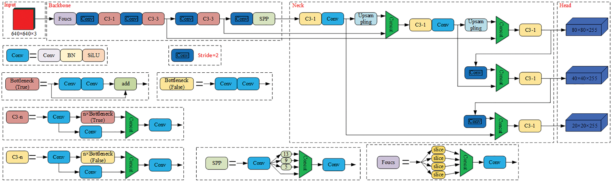
Figure 2: The network structure of YOLOv5s

The input comprises mosaic data augmentation, image size processing, and adaptive anchor box computation. Mosaic data augmentation increases the number of tiny items in the background and dataset by merging four photos, as shown in Fig. 3. Image size adaptive processing employs a minimum black boundary to scale the original image evenly and without distortion to a standard size. The adaptive anchor box computation compares the increased expression box with the actual box predicated on the starting anchor box and calculates the gap between them to determine the best anchor box value [30], after which it updates in the opposite direction.

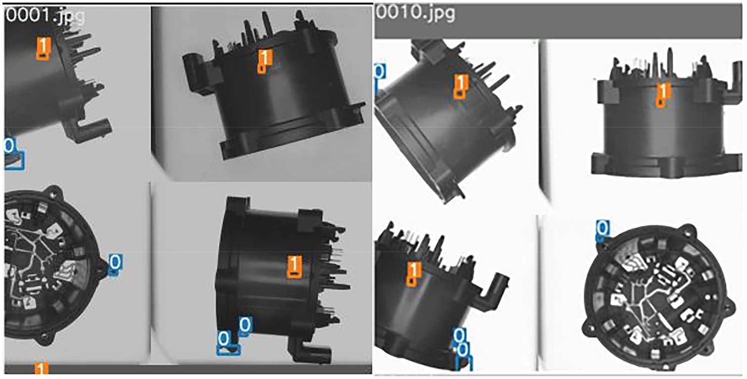
Figure 3: The electronic water pump shell mosaic data enhancement

The YOLOv5s backbone network is made up of modules such as Focus, Conv, C3, SPP, and others. The Focus module splits the picture data into four segments, each of which is downsampled two times. To create a new feature map with no information loss and size reduced by half, the data of all four are combined. The Focus module can minimize information loss and computation while increasing the diversity of difficult samples and data. Conv is the fundamental unit of convolution in YOLOv5s. The C3 module is made up of several structural modules known as bottleneck residuals. The SPP module uses different kernel sizes to perform maximum pooling and fuses features by connecting them [31].

The neck network is primarily in charge of feature augmentation and enhances the features that are taken from the backbone network to increase the accuracy of the subsequent predictions. The FPN and PAN pyramid structure is employed in the neck network [32,33]. The capacity of the neck network to fuse features is improved by combining these two structures.

The prediction network contains the target item’s category probability, object score, and bounding box position. The detection network has three detection layers and utilizes feature maps of various sizes to identify targets of various sizes. Each detection layer outputs related vectors, which are then used to create prediction bounding boxes and designate the various items in the original picture.

2.2 Improvement of YOLOv5s Network Architecture Design

2.2.1 MobileNet Lightweight Improvement

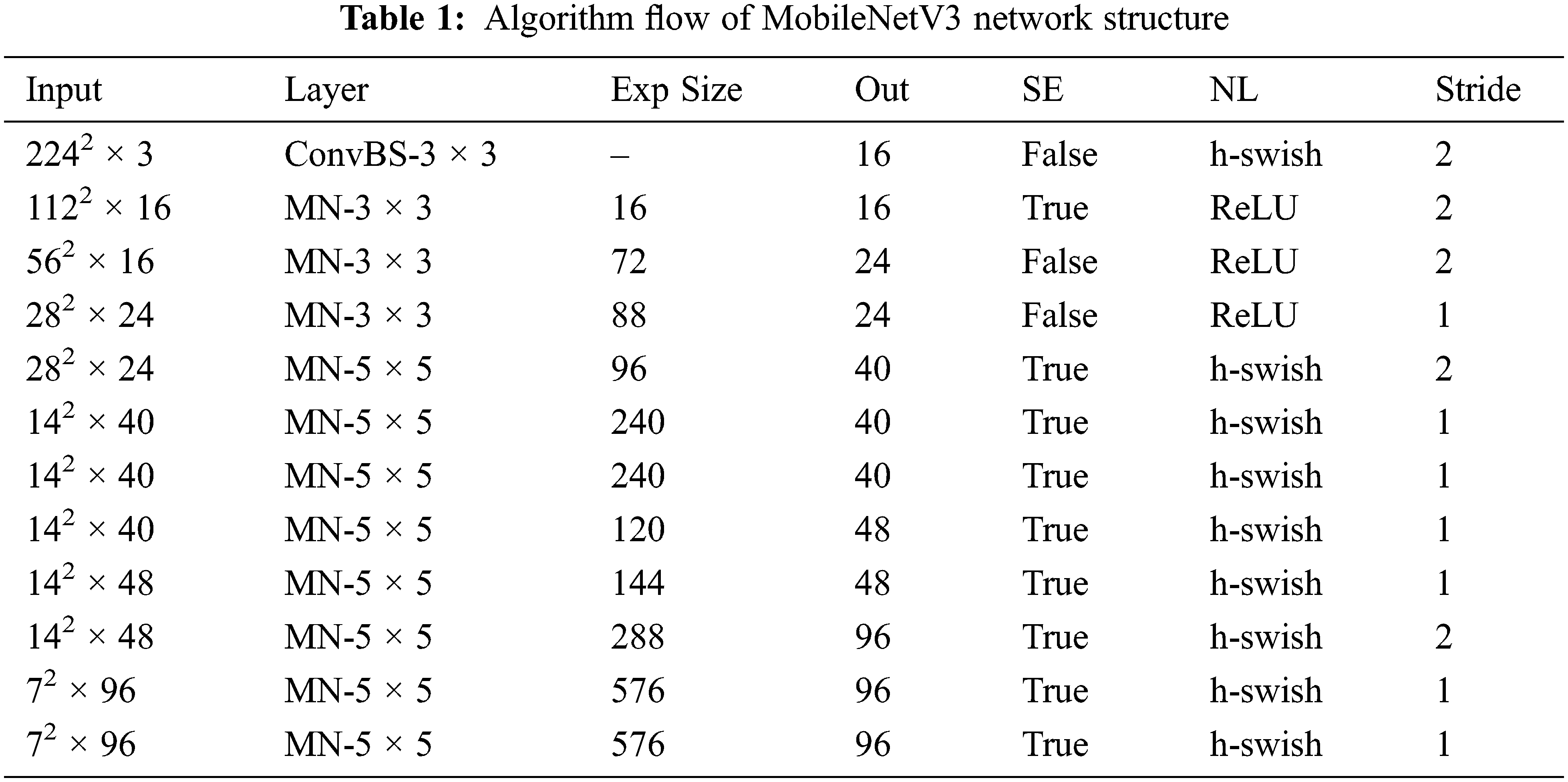
Real-time defect detection of electronic water pump shells requires a certain detection speed. YOLOv5 is a one-stage algorithm that meets the requirements of the experimental object. Thus, a lightweight network model based on YOLOv5s is developed for electronic water pump shell defect detection. The model uses the MobileNetV3 module instead of the original YOLOv5s backbone network structure, as shown in Fig. 4. In the backbone network of this method, the algorithm flow of the MobileNetV3 network structure is shown in Table 1. MobileNetV3 is separated into several phases, and SE modules are added to some of MobileNetV3’s bottlenecks. The key features of MobileNetV3 are its depth-separable convolution, reverse residual structure, and attention mechanism [34].

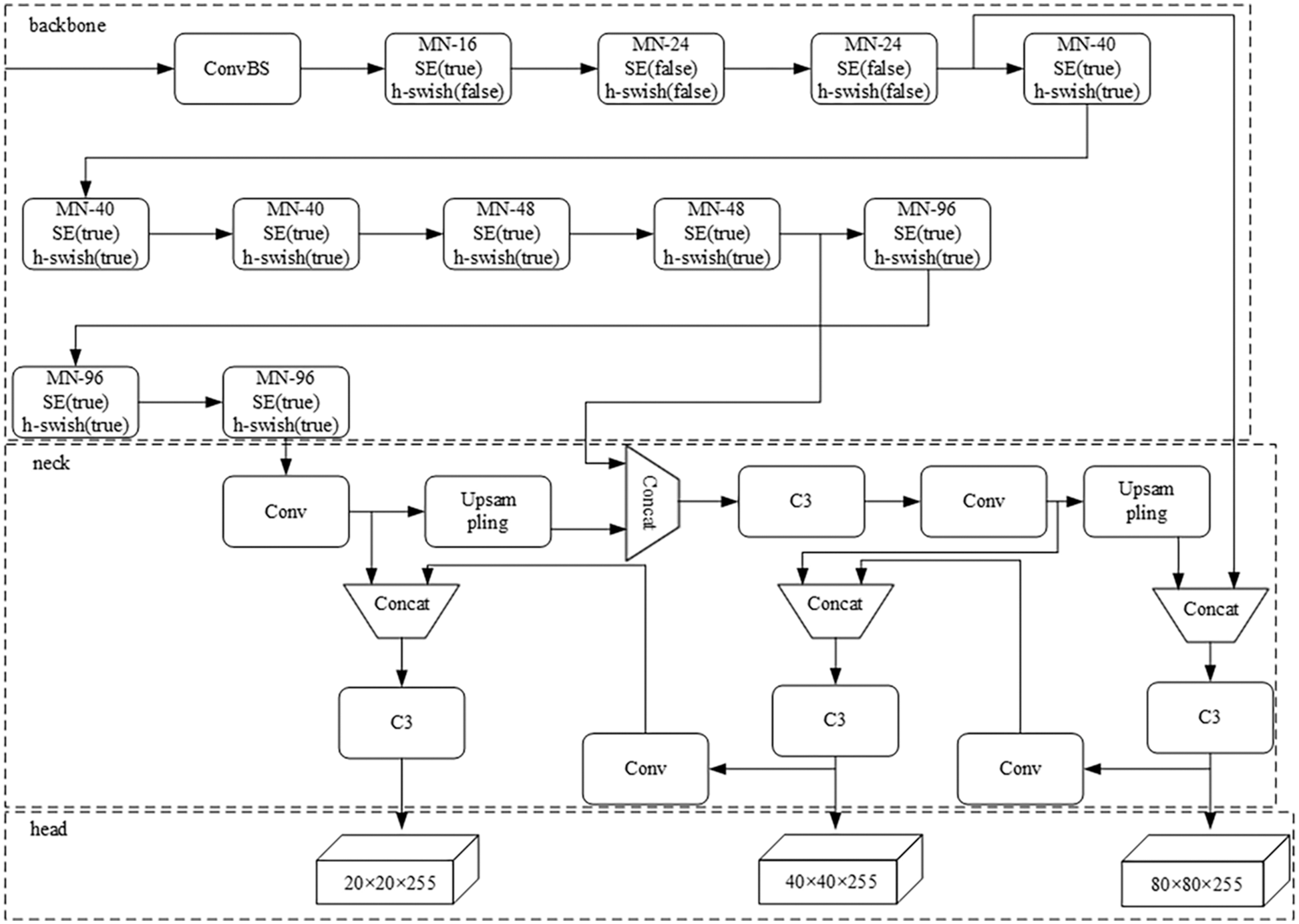
Figure 4: The improved YOLOv5s network structure

The backbone network consisting of MobileNet contains 13 convolutional layers, an average pooling layer, and a fully connected layer in addition to the input and output layers. Its core idea is deep-separable convolution, which converts ordinary convolution operations into 1 × 1 depthwise convolution and pointwise convolution. Depthwise convolution is used to extract information from each input channel, and pointwise convolution is used to linearly fuse multiple deep convolution outputs. Depth convolution only requires a single convolution kernel to extract features from each input channel. Because both depthwise and pointwise convolution use 1 × 1 convolution kernels, the number of computations and number of model parameters can be greatly reduced, thus increasing the overall speed of the network. Fig. 5 depicts the deep-separable convolution. The basic convolution kernel is shown in Fig. 5a, while the deep convolution kernel and the 1 × 1 point convolution kernel are shown in Figs. 5b and 5c, respectively.

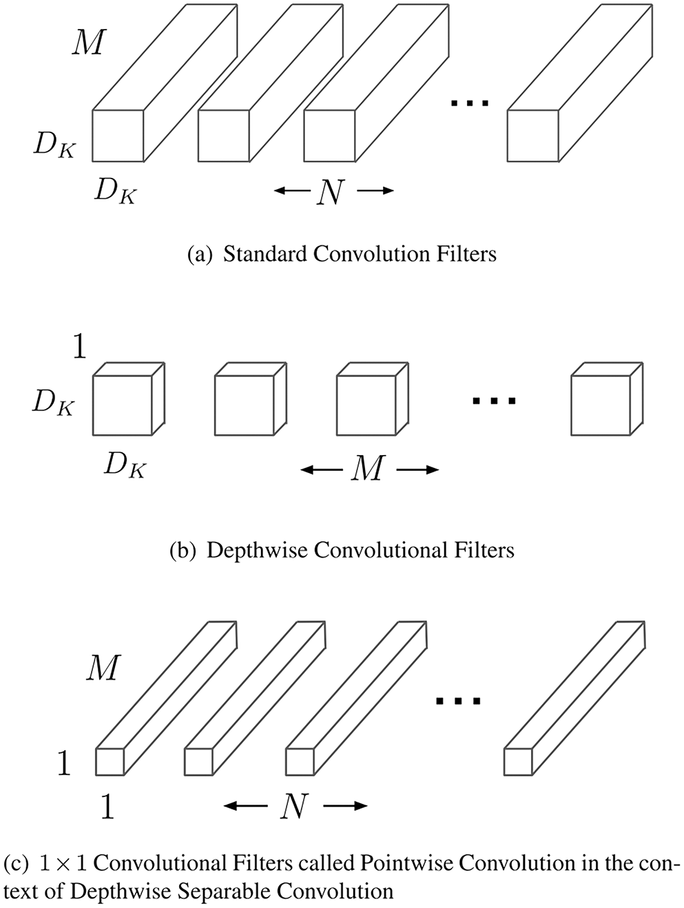
Figure 5: Schematic diagram of the depth-separable convolution

Theoretically, the impact of training increases as a network deepens. However, because of the difficulty of learning, an excessively deep network may degenerate in the actual operating process and thus be counterproductive. This flaw may be compensated for by using a reverse residual network. MobileNetV3 uses the V2 reverse residual structure. Compared with traditional residual networks, this structure has relatively few input channels. To train the network, the channel is first expanded, then its features are extracted and compressed. To increase the efficiency of memory utilization and gradient cross-layer propagation, shortcuts are introduced to the residual structure throughout this process.

The main design of MobileNetV3 incorporates the squeeze and excitation neural networks (SE-Net) [35], as shown in Fig. 6. By explicitly modeling the connection between network convolution feature channels, the main goal is to enhance the representation quality of network formation. In particular, learning is used to automatically determine the significance of each feature channel. This outcome leads to functional traits being enhanced while suppressing those that are not important for the task at hand.

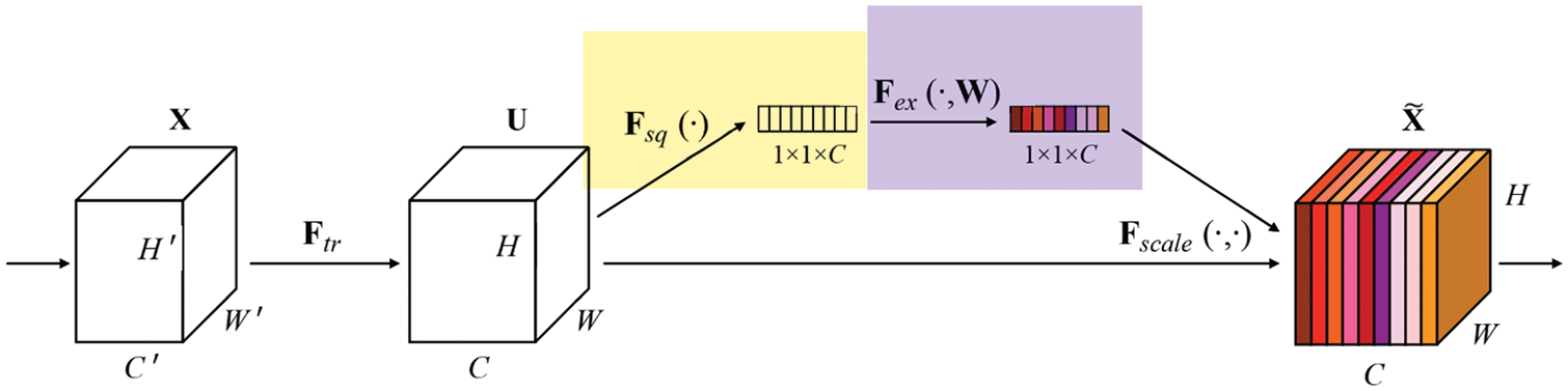
Figure 6: SE module structure diagram

The improved model uses depthwise separable convolution to reduce the number of parameters and FLOPs values. The reverse residual structure is used to improve the efficiency of gradient cross-layer propagation. Finally, the SE attention mechanism is used to improve the overall accuracy of the algorithm.

2.2.2 Loss Function Improvement

The YOLOv5 loss function includes confidence loss, classification loss, and target box and prediction box position loss. The total loss function is the combination of three losses expressed by:

Loss=lobj+lcls+lbox (1)

and the confidence loss function is as follows:

lobj=∑i=0s2∑j=0BIijobj(C^ilog⁡(Ci)+(1−C^i)log⁡(1−C^i))−λnoobj∑i=0s2∑j=0BIijnoobj(C^ilog⁡(Ci)+(1−C^i)log⁡(1−C^i)) (2)

where s2 represents the number of cells, B represents the number of predicted bounding boxes, Iijobj represents the object in the i-th cell and j-th bounding box, λnoobj represents a constant parameter, Ci and C^i represent the label and prediction of confidence of the bounding box predictor, respectively.

When calculating the classification loss for training, each label is exposed to the binary cross-entropy loss, which eliminates the use of the softmax function and reduces the computational complexity. The classification loss function is calculated as follows:

lcls=∑i=0S2lijabj∑c∈classes(P^i(c)log⁡(Pi(c))+(1−P^i(c))log⁡(1−Pi(c))) (3)

where Pi and P^ represent the probability values of the predicted and actual targets, respectively.

The GIoU_Loss function is employed in YOLOv5s to calculate the loss of the target box and prediction box positions [36]. The calculation is as follows:

lbox=LGIoU=1−(IoU−|C−(A∪B)||C|) (4)

where IoU represents the ratio of the intersection and union of the predicted bounding box and the labeled bounding box, A represents the area of the actual box, B represents the area of the predicted box, and C represents the area of the smallest external rectangle.

GIoU_Loss serves as the boundary box regression loss function in YOLOv5s. The loss function in IoU_Loss is not distinguishable when the prediction box and the target box do not intertwine—that is, when IoU = 0—thus making IoU_Loss impossible to optimize in the scenario in which the two boxes do not intersect. This problem is resolved by implementing the cross-scale measurement approach in GIoU_Loss. Additionally, IoU_Loss is unable to discriminate between prediction boxes at the juncture where they meet when they are the same size and have the same IoU. However, because the various kinds of prediction boxes and target boxes are identical, GIoU_Loss cannot handle the situation of the prediction box being inside the target box and both box sizes being the same.

Therefore, this paper will use CIoU_Loss as the regression loss function of the target detection task [37]. The formula is as follows:

LCloU=1−IoU+ρ2(b,bgt)c2+αv (5)

where b , bgt respectively represents the center points of the prediction box and the target box, ρ is the euclidean distance, c represents the diagonal distance between the minimum closure region of the prediction box and the target box, α represents the weight function, v represents the mixing degree of the aspect ratio between the anchor and target boxes. The calculation is shown in Eqs. (6)–(7).

α=v(1−IoU)+v (6)

v=4π2(arctanωgthgt−arctanωh)2 (7)

In contrast to GIoU_Loss, CIoU_Loss considers the distance between the center point, the aspect ratio of the bounding box, and the scale information of the overlap region between the prediction box and the target box. To increase the bounding box regression’s stability and convergence speed, CIoU_Loss is used as the loss function.

2.3 Evaluating Indicator

This article assesses the effectiveness of the improved experimental model using precision, recall, mAP@0.5, mAP@0.5:0.95, average detection processing time, parameter amount, FLOPs, and model size. The precision is calculated as the ratio of accurately guessed positive samples to specimens that were predicted to be positive samples as follows:

Precision=TPTP+FP (8)

and the recall rate is determined by taking the proportion of all correctly predicted targets and dividing it by the number of targets as follows:

Recall=TPTP+FN (9)

where TP denotes the number of correctly identified defective samples, FP denotes the number of incorrectly identified qualified samples, and FN denotes the number of incorrectly identified defective samples.

The equations for mAP@0.5 and mAP@0.5:0.95 are shown in Eqs. (10)–(11).

AP=∫01P(R)dR (10)

mAP=1N∑i=1NAPi (11)

mAP@0.5 is the mean AP for all categories when IoU is set to 0.5 and mAP@0.5:0.95 is the mean AP at distinct IoU threshold values, with IoU values ranging from 0.5 to 0.95 and the number of iterations set to 0.05.

The average detection processing time includes system convergence speed and NMS processing time. The model size is set to the model size that was saved following the prior model training.

3  Experiments

3.1 DataSet

3.1.1 Acquisition Equipment Construction

In this experiment, a high-pixel camera is needed to obtain the surface details and the small defects of the electronic water pump shell. Thus, an area array industrial camera with a 5-megapixel CMOS image sensor is used. To collect clear images, the camera resolution is set to 2K. The platform for acquiring faulty features for bespoke datasets and the real-time detection test is shown in Fig. 7. The device includes an adjustable bracket for adjusting the camera and the upper light source for close-up photography of the electronic water pump shell. The upper and lower light sources are also important components for obtaining clear images of the defect surface area. The brightness of the light source can be adjusted according to the environmental conditions of the required exposure.

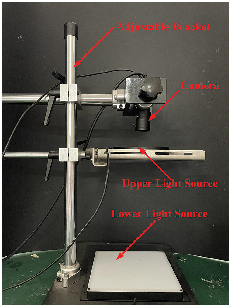
Figure 7: Image acquisition experimental platform

3.1.2 Image Capture and Processing

The dataset used in this experiment is from SUZHOU DITIAN ROBOT Co., Ltd. The electronic water pump shell is mainly produced by mold injection molding, which includes two kinds of surface defects: burrs and scratches. A total of 1423 images containing defects were collected. To create a larger dataset, each defect was enhanced using image enhancement techniques, such as brightness enhancement, horizontal flipping, and rotation, as shown in Fig. 8. The dataset was expanded to more than 5000 images for the training of the network model used in this paper. The training set: validation set: test set ratio is set to 7:2:1.

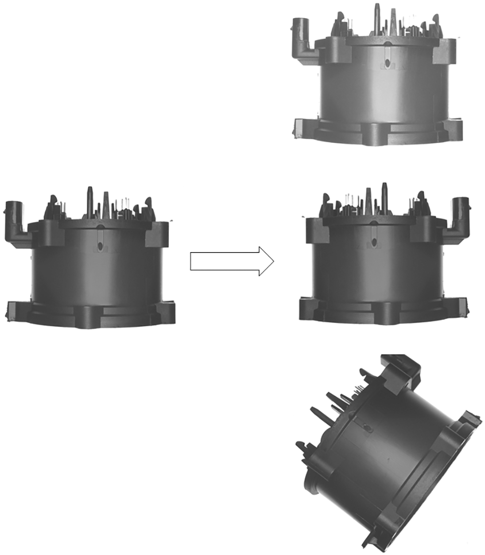
Figure 8: Image enhancement process diagram

We manually mark the custom dataset before training the model with the machine learning annotation tool. Make Sense software is employed to coordinate defect area locations and to identify defect types before exporting the .txt file that includes the training model. Fig. 9 depicts several tagging instances using Make Sense.

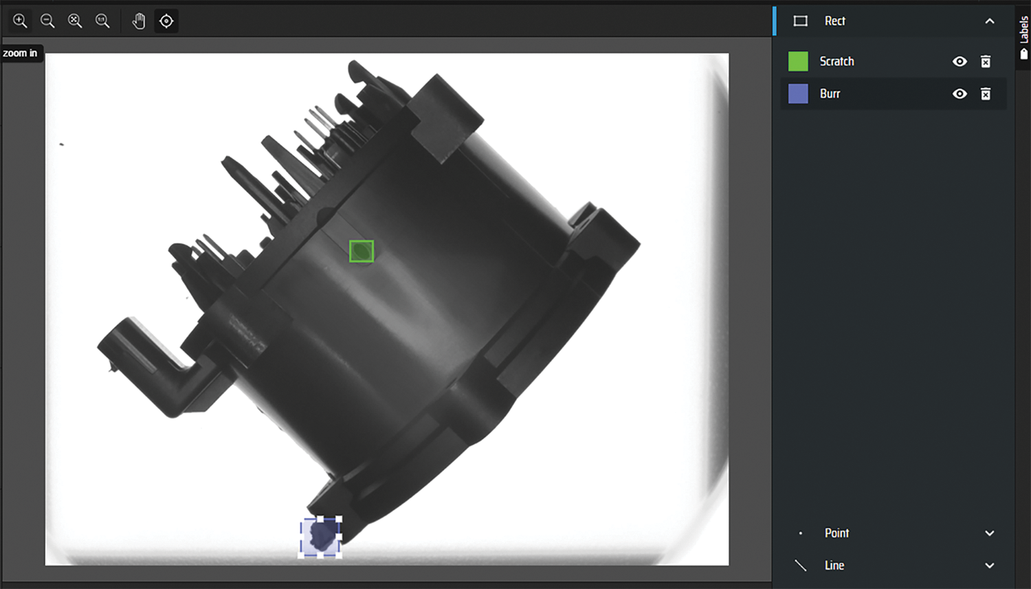
Figure 9: Make Sense software tag example

3.2 Experimental Configuration and Settings

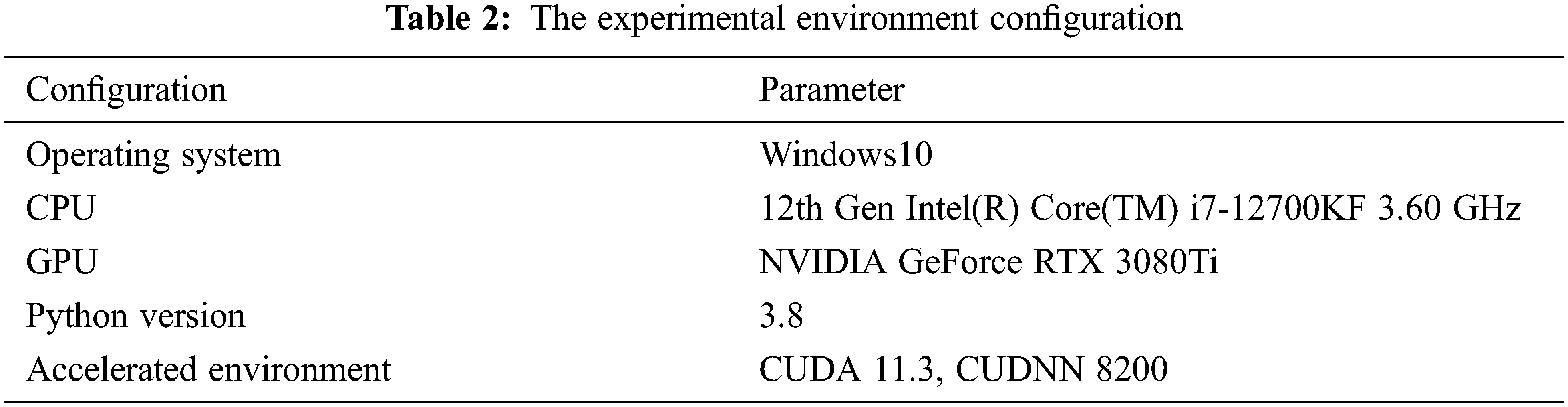
The construction, training, and testing of the experimental model in this paper are completed under the deep learning Pytorch framework using the Windows10 operating system. The specific experimental environment is shown in Table 2.

This experiment employs preheating training to preserve the deep stability of the model and to prevent model oscillation caused by the overly high initial learning rate during model training. The learning rate increases from 0 to the predetermined value of 0.01 during the preheating training phase. Following the warm-up stage [38], the learning rate is updated using the cosine annealing technique [39]. Fig. 10 depicts the particular variations in learning rate. To update and improve the network model’s weights, the stochastic gradient descent technique is utilized during model training. The specific parameters of the experimental training are set as follows: the image size is 640 × 640, the batch size is 32, the learning rate is 0.01, the momentum parameter is 0.937, the weight attenuation coefficient is 0.0005, and the maximum number of iterations is 200.

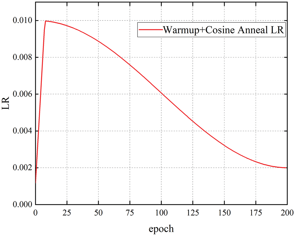
Figure 10: The learning rate change chart

3.3 Experimental Analysis

3.3.1 Experimental Analysis in Electronic Water Pump Shell Dataset

The effect of network structure changes on network performance was verified by conducting ablation experiments. In this paper, the model is contrasted with the initial results of YOLOv5s and YOLOv7_tiny, and the backbone model of YOLOv5s is improved in models that include YOLOv5s_CBAM, YOLOv5s_SE, and YOLOv5s_MobileNetV2. The results are shown in Fig. 11 and Table 3.

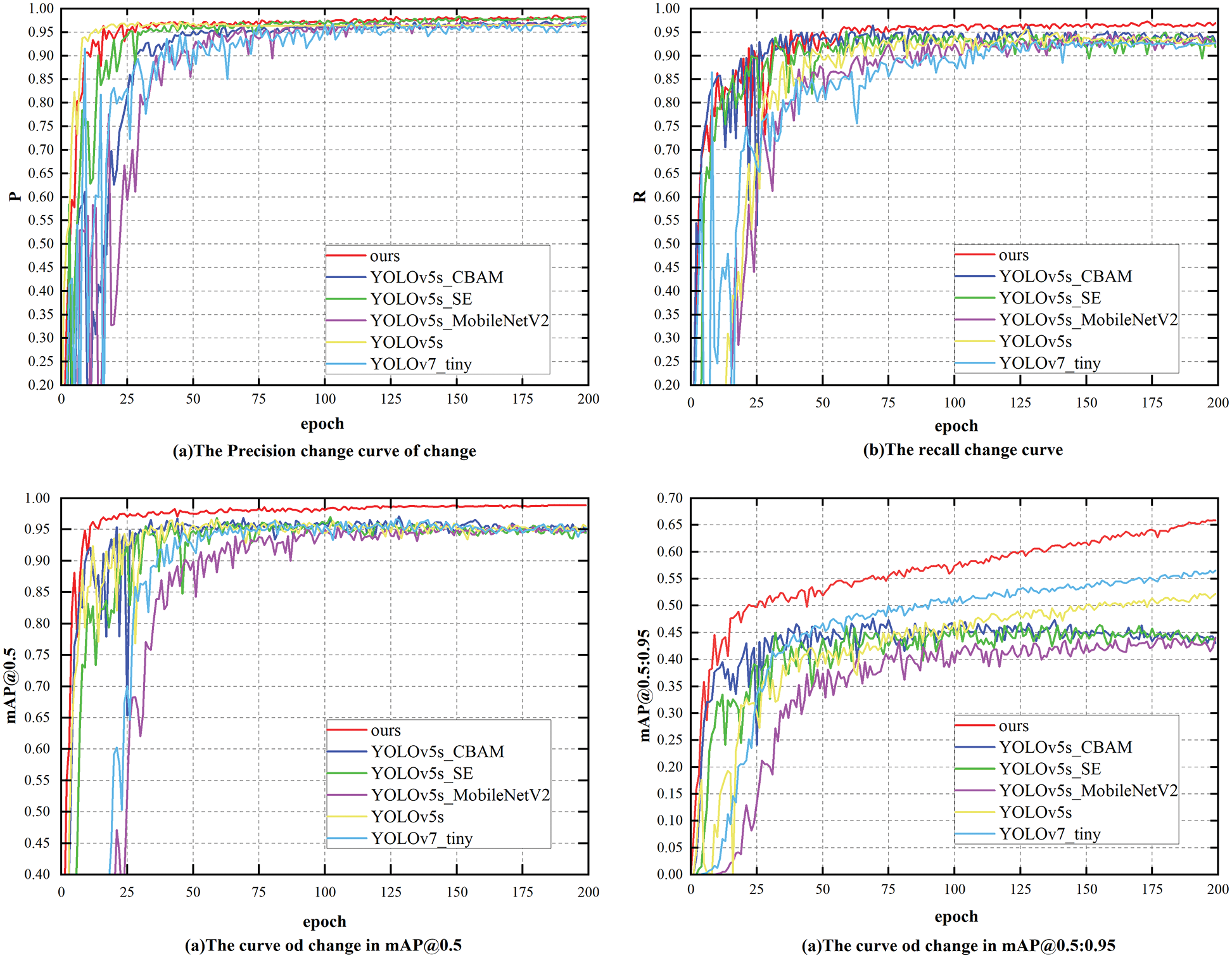
Figure 11: The comparison of the results of each model

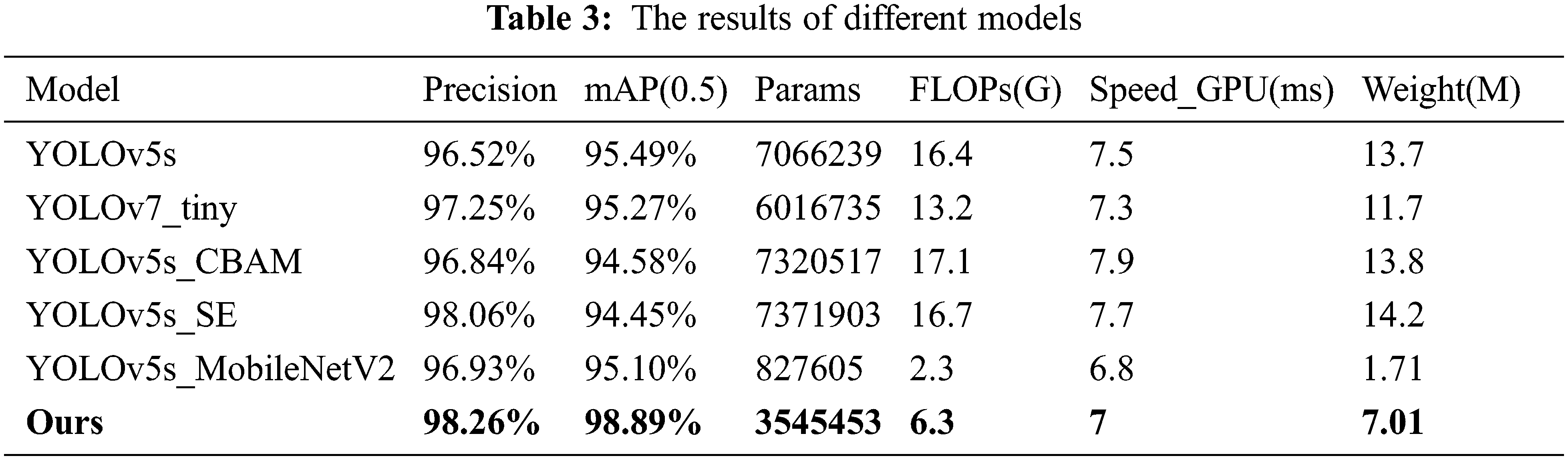
Fig. 11 shows the performance of each network structure we tested on the electronic water pump shell dataset, and the specific results are shown in Table 3. The results show that the training accuracy of the upgraded model is enhanced and that the average detection processing time is somewhat longer when the attention mechanism module (i.e., CBAM, SE) is added to the YOLOv5s backbone network. The FLOPs and model parameters are quite similar to those of YOLOv5s. The calculating cost is decreased and the processing speed is increased once the YOLOv5s backbone network is replaced with the MobileNetV2 module. When compared to YOLOv5s, the average detection processing time is 6.8 ms, the FLOPs and model parameters are lowered by 85.98% and 88.29%, respectively, and the model accuracy is somewhat improved. The model used in this paper adds the attention mechanism SE module to the MobileNet module to replace the YOLOv5s backbone network and uses CIoU_Loss instead of GIoU_Loss. The average detection processing time is not as fast as that of the YOLOv5s_MobileNetV2 model but reaches 7 ms. Compared with YOLOv5s, the FLOPs and the total number of model parameters in this study decreased by 61.59% and 49.83%, respectively, and the model accuracy increased by 1.74%. Compared with YOLOv7_tiny, the total number of FLOPs and model parameters decrease by 52.27% and 41.07%, respectively, and the model accuracy increases by 1.01%.

After training the model used in this paper and the YOLOv5s model, the optimal weight file is selected and the performance comparison is conducted using the test dataset of the electronic pump shell, as shown in Fig. 12. The left figure is the test result of YOLOv5s, and the right figure is the test result of the model used in this paper. As shown in Figs. 12a and 12b, the detection accuracy of the proposed model is higher than that of YOLOv5s in the detection of the original image and the top image. As shown in Figs. 12c and 12d, the detection accuracy of the model are greater than that of YOLOv5 s under the interference of brightness and blur. The results show that the proposed model is superior to the YOLOv5s model.

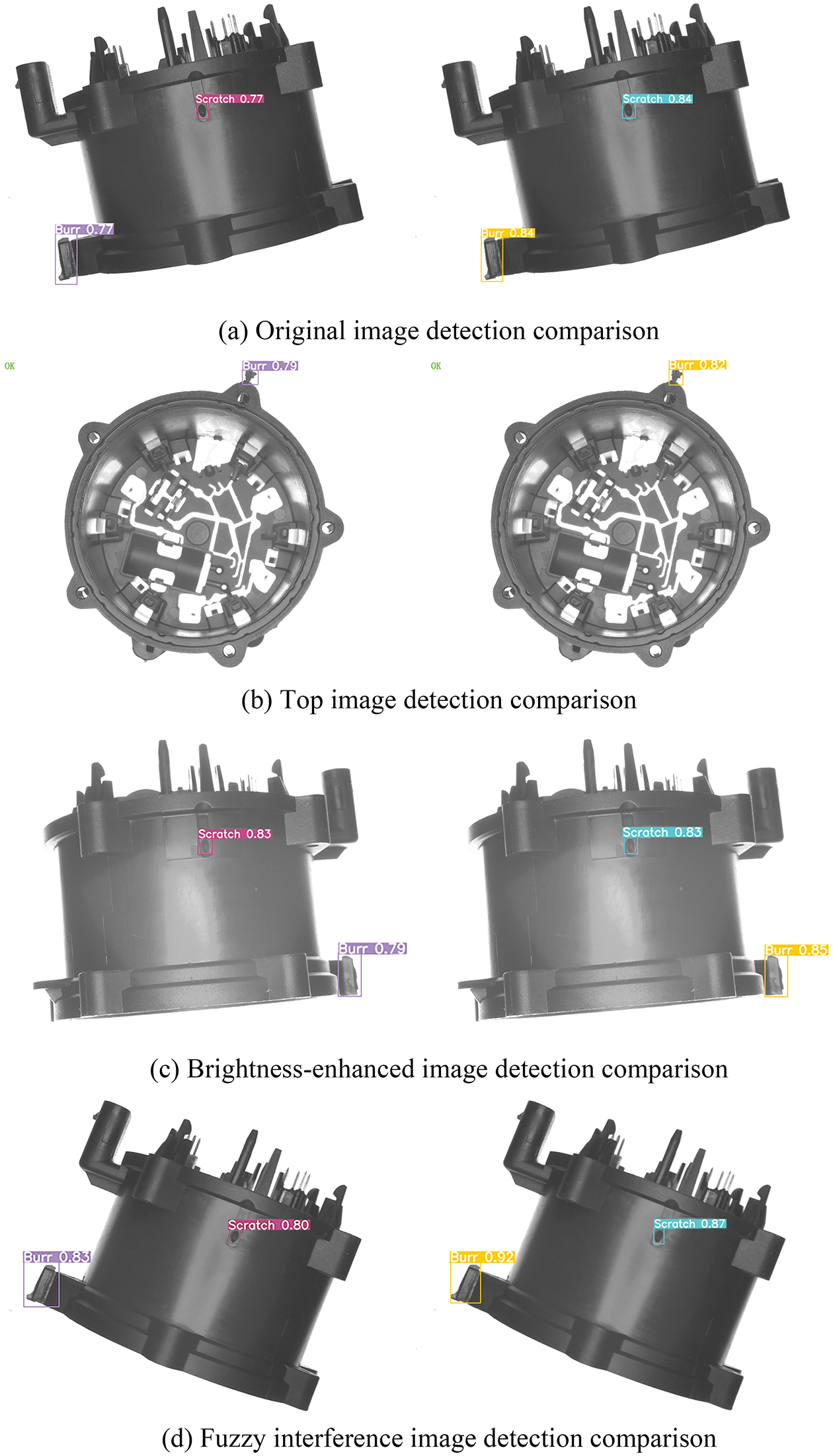
Figure 12: The comparison of multi-angle experimental results

3.3.2 Experimental Analysis in PASCAL VOC2007 Dataset

To further verify the superiority and applicability of the model used in this paper, some PASCAL VOC2007 datasets that include 15 target categories are used to verify the model.

The model results using PASCAL VOC2007 datasets are compared with those using YOLOv5s. The results are shown in Fig. 13 and Table 4. Compared with the YOLOv5s model, the training accuracy and detection accuracies are 84.16% and 80.78%, respectively, which represent increases of 4.37% and 2.19%, respectively. In addition, the model is smaller than the YOLOv5s model in terms of the number of parameters, FLOPs, and model size. The comparison of the consequences of the detection between the two models is shown in Fig. 14. The detection results for the suggested model are shown on the right, while the detection results for YOLOv5s are shown on the left. The results show that the model’s performance is nearly identical to that of YOLOv5s in real-life situations. However, the model outperforms YOLOv5s for tiny objects that require dense detection.

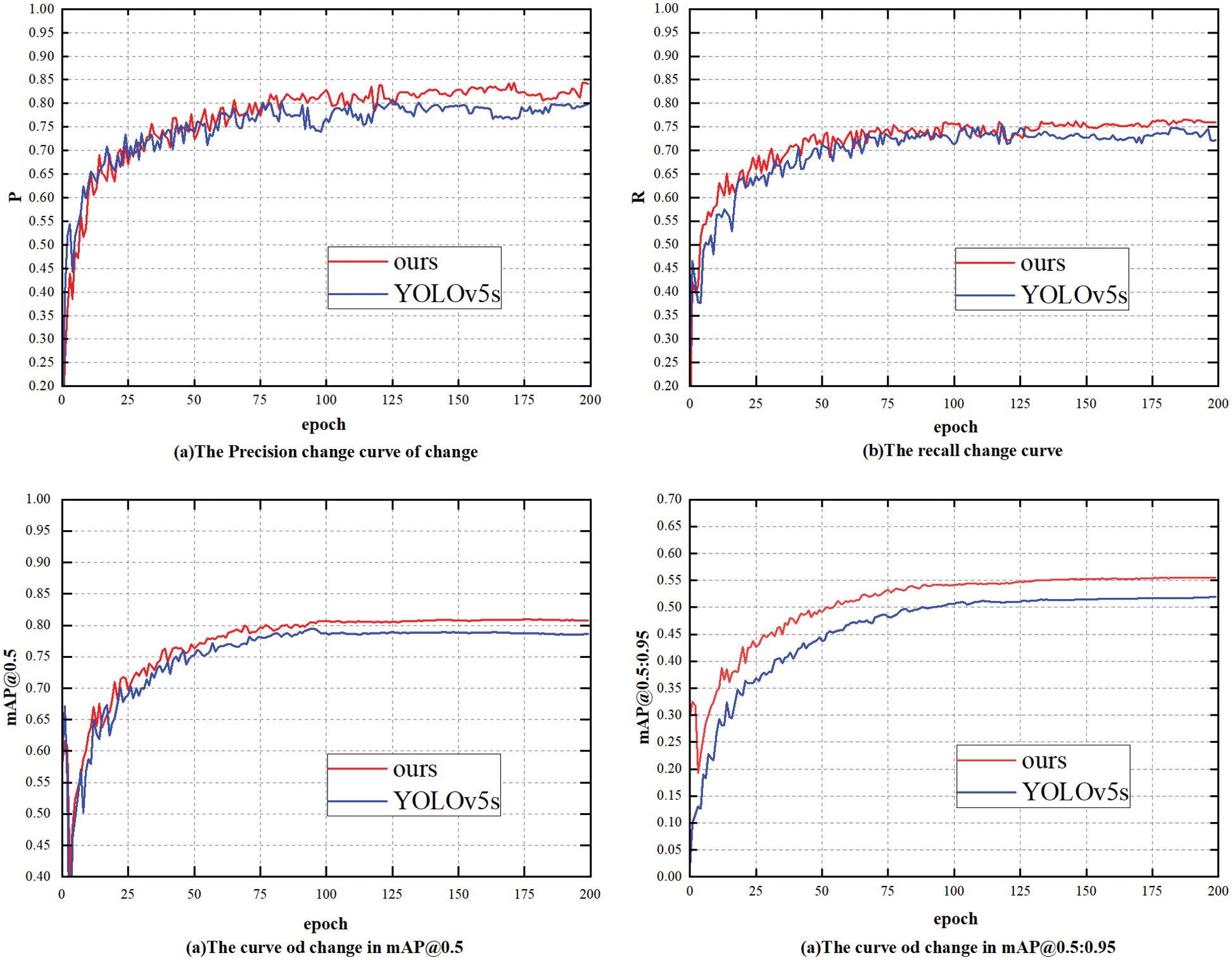
Figure 13: The comparison of experimental results in some PASCAL VOC2007 datasets

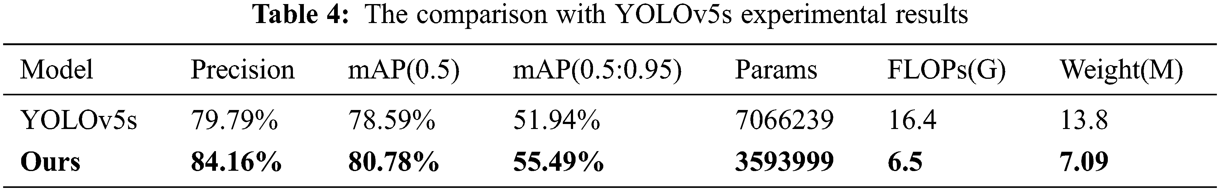
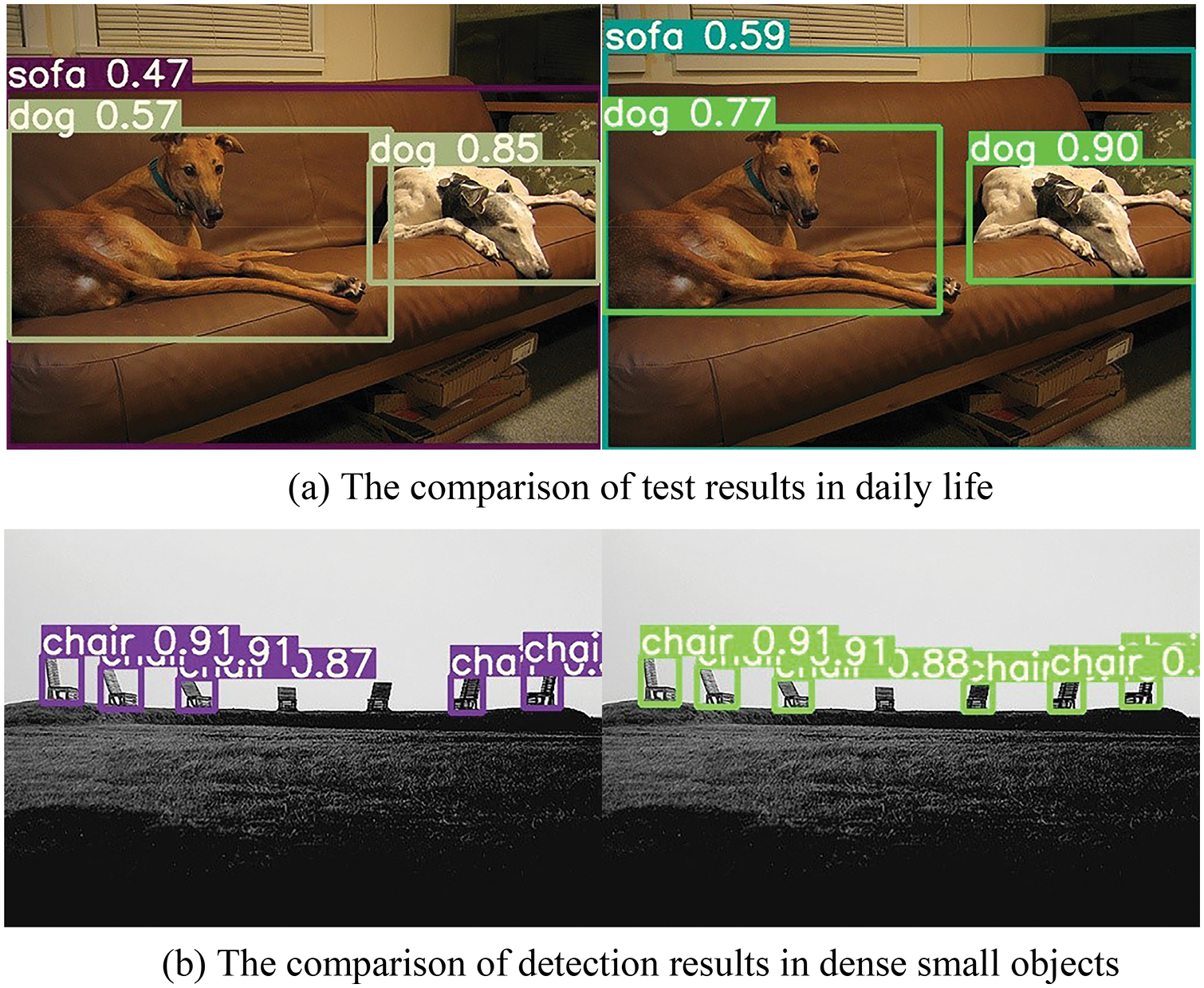
Figure 14: The comparison of detection results in some PASCAL VOC2007 datasets

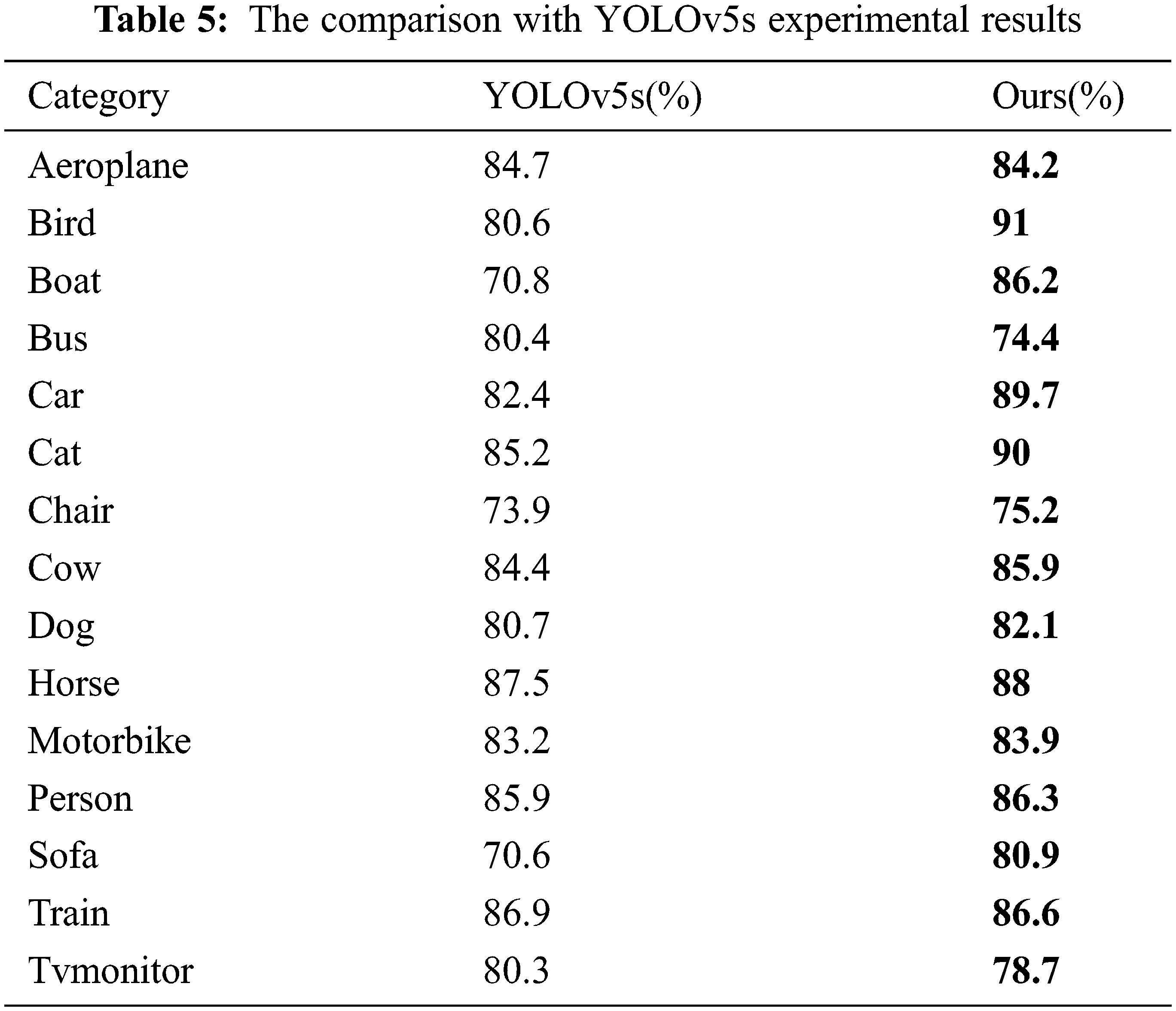
The outcomes of the single-class analysis between the model proposed in this paper and the YOLOv5s model on a segment of the PASCAL VOC 2007 test set are displayed in Table 5. The findings demonstrate that in 11 of the 15 categories, the model’s single-class precision values are greater than those of the YOLOv5s model. As a result, the method’s detection accuracy is higher than that of YOLOv5s. In multi-category target identification tasks, the model still outperforms YOLOv5s, thus demonstrating the adaptability of the proposed strategy.

4  Conclusion

In this paper, an improved lightweight network model based on YOLOv5s is proposed to detect electronic water pump shells in real-time. The MobileNetV3 network is used to replace the original YOLOv5s backbone network in extracting features from the image, which effectively reduces the number of parameters and calculations. CIoU_Loss is used in the bounding box loss function of the model to improve its accuracy. An image acquisition platform was built to collect images more quickly and effectively, and a dedicated electronic water pump shell dataset was created and verified on it. The results show that the detection accuracy and mAP (0.5) value of the electronic water pump shell reaches 98.26% and 98.89%, respectively, and the detection speed reaches 7 ms. The model has higher detection accuracy than YOLOv5s. It still has good performance in small targets and the presence of other types of interference. In addition, the model is used to verify its versatility on the PASCAL VOC2007 dataset, and it shows good detection performance for things observed in daily life. The model provides an effective method for the automatic real-time detection of surface defects in electronic water pump shells and thus completes the standardized intelligent automatic inspection of the product, reduces manual involvement, and greatly improves the automation level of the manufacturer.

In future work, we will strive to improve the model’s accuracy and speed by incorporating attention methods such as efficient channel attention and convolutional block attention modules.

Acknowledgement: The author would like to thank the automation department of Suzhou Ditian Robot Co., Ltd., for the equipment provided for this research.

Funding Statement: This work is supported by the Qing Lan Project of the Higher Education Institutions of Jiangsu Province, the 2022 Jiangsu Science and Technology Plan Special Fund (International Science and Technology Cooperation) (BZ2022029).

Conflicts of Interest: The authors declare that they have no conflicts of interest to report regarding the present study.

References

 1.  Y. LeCun, L. Bottou, Y. Bengio and P. Haffner, “Gradient-based learning applied to document recognition,” Proceedings of the IEEE, vol. 86, no. 11, pp. 2278–2324, 1998. [Google Scholar]

 2.  M. Riaz, H. M. A. Farid, H. M. Shakeel and D. Arif, “Cost effective indoor HVAC energy efficiency monitoring based on intelligent decision support system under fermatean fuzzy framework,” Scientia Iranica, Article 22785, 2022. https://doi.org/10.24200/SCI.2022.59197.6106. [Google Scholar]

 3.  K. Simonyan and A. Zisserman, “Very deep convolutional networks for large-scale image recognition,” Computer Science. arXiv preprint arXiv:1409.1556, 2014. [Google Scholar]

 4.  C. Szegedy, W. Liu, Y. Q. Jia, P. Sermanet, S. Reed et al., “Going deeper with convolutions,” in Proc. of the IEEE Conf. on Computer Vision and Pattern Recognition, Boston, MA, pp. 1–9, 2015. [Google Scholar]

 5.  K. He, X. Y. Zhang, S. Q. Ren and J. Sun, “Deep residual learning for image recognition,” in Proc. of the IEEE Conf. on Computer Vision and Pattern Recognition, Las Vegas, NV, USA, pp. 770–778, 2016. [Google Scholar]

 6.  X. Y. Chen, D. Y. Wang, J. J. Shao and J. Fan, “Plastic gasket defect detection based on transfer learning,” Scientific Programming, vol. 2021, article ID. 5990020, pp. 11, 2021. [Google Scholar]

 7.  B. Chakravarthi, S. C. Ng, M. R. Ezilarasan and M. F. Leung, “EEG-based emotion recognition using hybrid CNN and LSTM classification,” Frontiers in Computational Neuroscience, vol. 16, pp. 1019776, 2022. [Google Scholar]

 8.  A. K. F. Lui, Y. H. Chan and M. F. Leung, “Modelling of destinations for data-driven pedestrian trajectory prediction in public buildings,” in IEEE Int. Conf. on Big Data (Big Data), Orlando, FL, USA, pp. 1709–1717, 2021. [Google Scholar]

 9.  M. Riaz, H. M. A. Farid, H. M. Shakeel and Y. Almalki, “Modernizing energy efficiency improvement with q-Rung orthopair fuzzy MULTIMOORA approach,” IEEE Access, vol. 10, pp. 74931–74947, 2022. [Google Scholar]

10. Z. Y. Xing, Z. Y. Zhang and X. W. Yao, “Automatic image positioning of a rail train number using speed-up robust features and stroke width transform,” Proceedings of the Institution of Mechanical Engineers, Part C: Journal of Mechanical Engineering Science, vol. 236, no. 17, pp. 9871–9881, 2022. [Google Scholar]

11. J. Redmon, S. Divvala, R. Girshick and A. Farhadi, “You only look once: Unified, real-time object detection,” in Proc. of the IEEE Conf. on Computer Vision and Pattern Recognition, Las Vegas, NV, USA, pp. 779–788, 2016. [Google Scholar]

12. J. Redmon and A. Farhadi, “YOLO9000: Better, faster, stronger,” in Proc. of the IEEE Conf. on Computer Vision and Pattern Recognition, Honolulu, HI, USA, pp. 7263–7271, 2017. [Google Scholar]

13. J. Redmon and A. Farhadi, “Yolov3: An incremental improvement,” in Proc. of the IEEE Conf. on Computer Vision and Pattern Recognition, arXiv preprint arXiv: 1804.02767, 2018. [Google Scholar]

14. R. Girshick, J. Donahue, T. Darrell and J. Malik, “Region-based convolutional networks for accurate object detection and segmentation,” IEEE Transactions on Pattern Analysis and Machine Intelligence, vol. 38, no. 1, pp. 142–158, 2015. [Google Scholar]

15. R. Girshick, “Fast R-CNN,” in Proc. of the IEEE Int. Conf. on Computer Vision, Santiago, Chile, pp. 1440–1448, 2015. [Google Scholar]

16. S. Ren, K. He, R. Girshick and J. Sun, “Faster R-CNN: Towards real-time object detection with region proposal networks,” IEEE Transactions on Pattern Analysis and Machine Intelligence, vol. 39, no. 6, pp. 1137–1149, 2016. [Google Scholar]

17. W. Liu, D. Anguelov, D. Erhan and C. Szegedy, “SSD: Single shot multibox detector,” in European Conf. on Computer Vision, Amsterdam, The Netherlands, pp. 21–37, 2016. [Google Scholar]

18. C. Y. Fu, W. Liu, A. Ranga, A. Tyagi and A. C. Berg, “DSSD: Deconvolutional single shot detector,” in Proc. of the IEEE Conf. on Computer Vision and Pattern Recognition, arXiv preprint arXiv: 1701.06659, 2017. [Google Scholar]

19. J. Dai, Y. Li, K. He and J. Sun, “R-FCN: Object detection via region-based fully convolutional networks,” in Proc. of the 30th Int. Conf. on Neural Information Processing Systems, Barcelona, Spain, pp. 379–387, 2016. [Google Scholar]

20. Z. Y. Xing, Z. Y. Zhang, X. W. Yao, Y. Qin and L. M. Jia, “Rail wheel tread defect detection using improved YOLOv3,” Measurement, vol. 203, no. 8, pp. 111959, 2022. [Google Scholar]

21. Y. Li, J. Zhang, Y. Hu, Y. N. Zhao and Y. Cao, “Real-time safety helmet-wearing detection based on improved YOLOv5,” Computer Systems Science & Engineering, vol. 43, no. 3, pp. 1219–1230, 2022. [Google Scholar]

22. X. W. Yao, Z. Y. Xing, Z. Y. Zhang and A. D. Sheng, “The online monitoring system of pantograph slider based on 2D laser displacement sensors,” Measurement, vol. 194, no. 1, pp. 111083, 2022. [Google Scholar]

23. M. I. Bin Roslan, Z. Ibrahim and Z. A. Aziz, “Real-time plastic surface defect detection using deep learning,” in IEEE 12th Symp. on Computer Applications & Industrial Electronics, Penang, Malaysia, pp. 111–116, 2022. [Google Scholar]

24. D. Tabernik, S. Sela, J. Skvarc and D. Skocaj, “Segmentation-based deep-learning approach for surface-defect detection,” Journal of Intelligent Manufacturing, vol. 31, no. 3, pp. 759–776, 2020. [Google Scholar]

25. J. J. Xing and M. P. Jia, “A convolutional neural network-based method for workpiece surface defect detection,” Measurement, vol. 176, no. 1, pp. 109185, 2021. [Google Scholar]

26. C. C. Ho, M. A. B. Hernandez, Y. F. Chen, C. J. Lin and C. S. Chen, “Deep residual neural network-based defect detection on complex backgrounds,” IEEE Transactions on Instrumentation and Measurement, vol. 71, no. 5005210, pp. 1–10, 2022. [Google Scholar]

27. Y. Q. Lu, B. Yang, Y. C. Gao and Z. M. Xu, “An automatic sorting system for electronic components detached from waste printed circuit boards,” Waste Management, vol. 137, no. 10, pp. 1–18, 2022. [Google Scholar]

28. H. Lee and K. Ryu, “Dual-kernel-based aggregated residual network for surface defect inspection in injection molding processes,” Applied Sciences, vol. 10, no. 22, pp. 8171, 2020. [Google Scholar]

29. G. Jocher, “Yolov5,” 2020. [Online]. Available: https://doi.org/github.com/ultralyc-s/yolov5. [Google Scholar]

30. X. D. Dong, S. Yan and C. Q. Duan, “A lightweight vehicles detection network model based on YOLOv5,” Engineering Applications of Artificial Intelligence, vol. 113, no. 1, pp. 104914, 2022. [Google Scholar]

31. K. He, X. Y. Zhang, S. Q. Ren and J. Sun, “Spatial pyramid pooling in deep convolutional networks for visual recognition,” IEEE Transactions on Pattern Analysis and Machine Intelligence, vol. 37, no. 9, pp. 1904–1916, 2015. [Google Scholar]

32. S. Liu, L. Qi, H. Qin, J. Shi and J. Jia, “Path aggregation network for instance segmentation,” in Proc. of the IEEE Conf. on Computer Vision and Pattern Recognition, Salt Lake City, UT, USA, pp. 8759–8768, 2018. [Google Scholar]

33. T. Y. Lin, P. Dollar, R. Girshick, K. He, B. Hariharan et al., “Feature pyramid networks for object detection,” in Proc. IEEE Conf. Computer Vision Pattern Recognition, Honolulu, HI, USA, pp. 936–944, 2017. [Google Scholar]

34. A. Howard, M. Sandler, B. Chen, W. J. Wang, L. C. Chen et al., “Searching for MobileNetV3,” in IEEE/CVF Int. Conf. on Computer Vision, Seoul, Korea (Southpp. 1314–1324, 2019. [Google Scholar]

35. J. Hu, L. Shen, S. Albanie, G. Sun and E. Wu, “Squeeze-and-excitation networks,” in Proc. of the IEEE Conf. on Computer Vision and Pattern Recognition, Salt Lake City, UT, USA, pp. 7132–7141, 2018. [Google Scholar]

36. H. Rezatofighi, N. Tsoi, J. Y. Gwak, A. Sadeghian, L. Reid et al., “Generalized intersection over union: A metric and a loss for bounding box regression,” in Proc. of the IEEE/CVF Conf. on Computer Vision and Pattern Recognition, Long Beach, CA, USA, pp. 658–666, 2019. [Google Scholar]

37. Z. H. Zheng, P. Wang, W. Liu, J. Z. Li, R. Ye et al., “Distance-IoU Loss: Faster and better learning for bounding box regression,” in Proc. of the AAAI Conf. on Artificial Intelligence, New York Hilton Midtown, New York, New York, USA, vol. 34, pp. 12993–13000, 2020. [Google Scholar]

38. R. Xiong, Y. C. Yang, D. He, K. Zheng, S. X. Zheng et al., “On layer normalization in the transformer architecture,” in Int. Conf. on Machine Learning, PMLR, pp. 10524–10533, 2020. [Google Scholar]

39. I. Loshchilov and F. Hutter, “SGDR: Stochastic gradient descent with warm restarts,” in Int. Conf. on Learning Representations, arXiv preprint arXiv: 1608.03983ol, 2016. [Google Scholar]