Earlier Detection of Alzheimer’s Disease Using 3D-Convolutional Neural Networks

1  Introduction

Alzheimer’s disease is determined as the influencing kind of dementia in the medical field. Generally, AD occurrence is identified for individuals aged 65 years (5%) and 30% for people above 85 years [1]. Based on the analysis reported by the World Health Organization (WHO), it is stated that 0.65 billion people will be diagnosed with AD in the later 2050 [2]. AD leads to the destruction of brain cells which directly influences people by losing mental function, memory, and inability to continue their daily-life activities. AD affects the brain parts and rules over memory and language [3]. As an outcome, AD patients are noted with confusion, memory loss, and complexity in writing, reading and speaking. Often, they seem to forget their lives and cannot identify their family members. Also, AD affected people suffer from carrying out their daily activities like combing hair and brushing teeth. These consequences make them aggressive, anxious, and wander over their home [4]. Therefore, it ultimately leads to the brain being destroyed and manages the heart’s functionality and control of breathing which causes death [5].

There are three diverse kinds of AD. They are: very mild, mild, and moderate. The AD prediction process is not proper until the patients reach the intermediate stage. Some essential things like neuro-biological and physical examinations, patients’ detailed history and Mini-Mental state examination (MMSE) are required for proper medical investigations on AD [6]. In recent times, physicians have been using Magnetic Resonance (MR) images to predict AD. It reduces the cerebral cortex, and the brain hippocampus expands ventricles. The hippocampus is generally accountable for spatial memory and episodic [7]. Also, it works as a relaying structure among the brain and body. The hippocampus reduction leads to damaged cells and influences the neuron ends and synapses. Therefore, neurons cannot establish communication through synapses anymore [8]. As an outcome, the brain parts related to the remembering portion (i.e., short-term memory like planning, thinking, and judging ability are affected [9]. The degraded brain tissues show lower MR image intensity. The researchers have modelled various computer-aided diagnostic systems to predict the disease correctly. In the earlier 1990s, the investigators modelled rule-based expertise systems and supervised models [10]. From their investigation, feature vectors are extracted from the provided image data for training the supervised methods, and the extraction of these features requires human experts with higher cost computation. With the emergence of deep learning approaches, features are extracted directly from the images, devoid of any human expert involvement [11]. Therefore, investigators concentrate on modelling and efficient DL approaches for appropriate disease diagnosis. This technological advancement has triumphed for various medical image analyses like mammography, X-ray, ultrasound, CT, microscopy, and MRI [12]. The deep learning models have shown pre-dominant outcomes for sub-structure and organ segmentation, various disease predictions and classification in the retina, breast, bone, cardiac, abdomen, lung, brain, pathology, and [13].

During the disease progression, abnormal proteins like hyperphosphorylated and amyloid- β are accumulated in the brain region of AD patients [14]. The accumulation of these abnormal proteins leads to synaptic progressive axonal and neuronal damage. The variations accounted in the brain region are due to AD with stereotypical patterns for earlier prediction of medial temporal lobe involvements (hippocampus and entorhinal cortex) followed by progressive neo-cortical damage. It shows some toxic effects on amyloid- β and hyperphosphorylated tau may gradually erode the brain regions, the clinical threshold is exceeded, and amnestic signs commence to grow. These changes happen before the appearance of the AD symptoms. Generally, structural MRI (sMRI) is considered for evaluating progressive brain variations because of AD [15]. The experimental outcomes examine the sMRI with DL approaches for AD prediction.

Various Machine Learning (ML) approaches are adopted for neuro-imaging data for constructing the diagnostic tools which assist in the automated classification and segmentation of brain MRI. Most learning approaches use handcrafted feature extraction and generation from the MRI data. These features are provided as the input to methods like Support Vector Machine (SVM), Logistic Regression (LR), Naïve Bayes (NB), and disease prediction. The knowledge experts perform a substantial role in the modelling of design architecture. However, neuro-imaging studies involve datasets with constraint samples. The image classification dataset performs object classification with huge images. For instance, the ImageNet dataset is a neuro-imaging dataset composed of hundreds of images. However, huge samples are required to construct feasible and robust neural networks. The lack of huge samples makes designing a model to learn the vital features from the smaller dataset essential. However, the prevailing DL approaches are optimized to work over the raw image data. Also, these models necessitate a vast amount of balanced training data to prevent network over-fitting. Here, a novel 3D-CNN model is used to learn the features from the online available ADNI dataset and eliminate the handcrafted feature extraction. It is trained using the ADNI dataset composed of 294 cognitively normal, 232 progressive Mild Cognitive Impairment (MCI), 254 stable mild cognitive impairments, and 268 AD samples. Our model predicts AD and outperforms all the existing approaches. The application relies on extending the hands to the medical community. Therefore, the below section shows the primary contributions of the work:

Here, the input is taken from the online source, i.e., ADNI dataset with huge samples and is well-suited to perform the DL classification process.

To design a novel 3D CNN for performing the classification and generating the outcomes. The model acts as a predictor approach to help the physicians during times of complexity.

The efficient approach is being trained to handle the over-fitting issues and evaluate various metrics like prediction accuracy, precision, recall and F1-score.

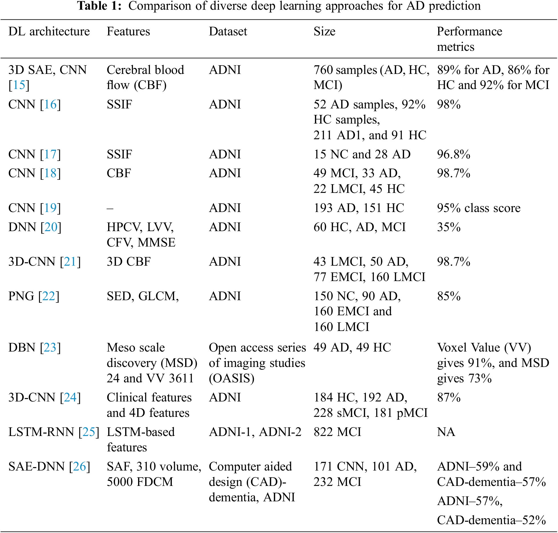
The remainder of the work is structured as follows: Section 2 provides an extensive review of the various existing approaches used for AD prediction and the pros and cons. Section 3 gives a detailed description of the anticipated 3D-CNN model for AD prediction with the later structure. In Section 4, the numerical results attained with the anticipated model are provided, and a detailed analysis is done with various existing approaches to show the model’s superiority. In Section 5, the research summary is given with certain research constraints and ideas for future research enhancements.

2  Related Works

AD is characterized based on the variations in mental degradation, which generally occurs for old-aged people due to the brain regions’ deterioration. Moreover, the investigators pretend to find the primary cause of the degradation and automated ways to predict neuroimages degeneration. Zhang et al. [16] discuss the DNN-based model composed of CNN and sparse AE using 3D convolutions of the entire MR images. The author acquired satisfactory outcomes by adopting 3-way classifier models like AD, MCI, and HC and attains a prediction accuracy of 89% and three binary classifications. Here, local 3D patterns are captured with the 3D-CNN model and acquire better outcomes than 2D convolutions. The experimentation over the convolutional layers is pre-trained using encoders, and it is not well-tuned to enhance classification performance. Moradi et al. [17] show the differentiation among AD and health control by scale extraction and shift-invariant among the lower to higher-level features using CNN. Here, a pipelined workflow is performed with sMRI data with a prediction accuracy of about 99%, and Functional Magnetic Resonance Imaging (fMRI) shows 98%. Initially, pre-processing is performed by the author to eliminate data distortion and noise. Next, CNN architecture comprises learning filters, scale-invariant operations, shift serving, and low-to-mid level features. GoogleNet and LeNet are executed in the successive pipeline to train and test the vast amount of images from 4D fMRI. The anticipated model shows higher prediction accuracy with better reproducibility. The author makes a significant contribution to multi-modal MRI bio-markers. The major constraint is that the experimentation is performed only for the people of fixed age by restricting the computation to explore the patterns of various age groups.

Zhao et al. [18] use CNN to predict AD from the health control. It performs scale-invariant and shifts features for feature extraction, followed by the LeNet model. It serves only binary image classification, and the accuracy attained with this is 96%. Ramírez et al. [19] model a framework with hyper-parameters from a deep image classifier model with CNN for predicting the stages of AD. Therefore, the anticipated model avoids the requirement for handcrafted features, which transforms the input towards the output by constructing the hierarchical feature from the lower-level features to higher-level features (complex). The anticipated model is adopted with hyper-parameters from deep classifiers, learning from image datasets. It predicts AD and classification with DL approaches over available datasets above 20 years. Here, the attained classification accuracy is 74% with a 5-fold Cross Validation (CV). Moreover, the author does not show much interest in validating the performance metrics compared to conventional approaches. El-Sappagh et al. [20] use CNN for multi-class classification among the Head Circumstance (HC), AD, and prodromal AD stages. The author designs the CNN model with MRI image pre-processing and attains grey matter images, and the latter discusses the CNN model. ResNet and GoogLeNet are used to train and test CNN. The author shows 4% improved prediction accuracy compared to other approaches, and the overall prediction accuracy is 98% for three classes, Non-Cognitive (NC), MCI and AD. McKhann [21] discuss various parameters attained from the 3D-CNN model for predicting MCI to AD with HC and AD classification. It relies on 3D clustered and separated convolutions for provisioning descriptive features from sMRI. Here, the author contributes to MCI prediction over the risky high convergence to AD in the earlier stage. The classification accuracy attained with this model is 87%, 86% sensitivity, and 86% specificity over a 10-fold CV. The parameters are evaluated efficiently by restricting over-fitting and exploiting HC and AD data. Afzal et al. [22] intend to classify HC and AD using layer-wise propagation over MRI data, compare the back-propagation with LRP, and perform appropriate detection. Also, it is reported that the approach is beneficial for clinical context and the constraint with this approach is the restricted ground-truth value. The approximation is used for dominating the classifier decision. The model highlights the significant contributions of the classifier model and does not facilitate assertion regarding the causes. It reports a 75% success rate and AD classification using a 5-fold CV. Altaf et al. [23] apply CNN for differentiating AD, MCI to AD and stable MCI for cross-sectional MRI scans. The model successfully overcomes the generalization constraints and performs various scanners, centres, and neuro-imaging protocols to acquire reproducibility and reliability. Some drawbacks could not exclude the functionality of MCI, and it has to be tested to enhance the prediction ability of that specific approach. The validation has to be performed in Positron emission tomography (PET), cognitive, clinical and genetic biomarkers. Choi et al. [24] conducted some modifications over the CNN layer and intended to predict dementia and AD using MR images. It is used to generalize other diseases, and the training process improves the prediction accuracy. The accuracy was attained at 81% using cross-validation. Gao et al. [25] anticipated conventional ML approaches like RF for feature selection and DNN for AD classification at the earlier stage. Here, the Kaggle dataset attains an overall accuracy of 35% using a 10-fold CV. The outcomes with DNN acquire appropriate prediction with the participant roaster, and the multi-class classification accuracy can compete with the clinical applicability.

Brier et al. [26] discuss LSTM with AE, which contains RNN for learning informative and compact representation from cognitive measures by facilitating and characterizing AD prediction with MCI progression. The model attains notable performance for MCI prediction to AD with two years follow-ups. The model is constructed with time points and gives superior performance to other models. The C-index acquired by the model is 90.1% with Alzheimer’s Disease Neuroimaging Initiative (ADNI)-1% and 88.9% with ADNIGO-2. Cox et al. [27] discuss an automatic AD prediction model with CNN using 3D MRI brain data by considering the entire 3D brain topology. CNN architecture comprises three consecutive groups with two FC layers and classification layers. Here, 3D brain topology is considered for the whole AD recognition, which improves prediction accuracy with a specificity of 93% and sensitivity of 100%. Kong et al. [28] discuss DNN with stacked-AR with multi-class classification and learns the complex non-linear patterns for MCI, NC, and AD classification. There are two specifications for blind datasets. The author produces a True Positive Rate (TPR) of 63% for AD, 55% for CN and 40% for MCI, and for the successive model, the TPR of AD is 65%, CN is 56% and 52% for MCI. Here, a superior fractal-based fractal dimensional co-occurrence is merged with surface area, cortical thickness, and volumetric analysis for multi-class AD classification. Sukkar et al. [29] anticipate a novel Markov model for automatic feature learning and predict AD fine-tuned and pre-processed using Markov. The model intends to predict the consequences of hyper-parameter analysis based on the AD classifier performance using preliminary models like pre-processing, data partitioning, and dataset size. The work concentrates on evaluation with data partitioning tests. Noh et al. [30] perform statistical analysis with a feature grey-level co-occurrence matrix based on Probabilistic Neural Network (PNN) and Principal Component Analysis (PCA) for training and classification. The author intends to classify NC, MCI, and AD. It attains 86% sensitivity, 83% specificity, and 86% accuracy, and the anticipated network model acquires superior outcomes than k-Nearest Neighbourhood (k-NN) and Support Vector Machine (SVM) based on accuracy.

There are two diverse kinds of approaches used for classification purposes. Sun et al. [31] designed the aAD model to attain superior performance devoid of any feature extraction process, which is time-consuming. The anticipated model performs an MRI classification task and intends to select the initial image of all subjects to avoid the probable information. Here, various performance metrics like Region of curve (ROC), Area Under Curve (AUC), and prediction accuracy are evaluated using ResNet and VoxCNN model attains 88%±0.08 and accuracy of 79%±0.08 for VoxCNN and AUC of 87%±0.07 and prediction accuracy of 80%±0.07 for ResNet. The model achieves one-verse classification and shows superior prediction accuracy and outcomes multi-class classification process. The primary research gap is the adversarial noise over the neuro-images, reducing classification accuracy. Therefore, the elimination of this noise is considered a significant research challenge. Similarly, DL shows superior accuracy with a large dataset and drastically impacts the prediction process. However, high-resolution CNN models like 2D/3DCNN offer outstanding performance for multi-modal neuro-images. The model attains excellent results with larger training datasets with DL approaches, which are a massive obstacle to the application process. Some datasets are found to be rare and limited [30–37]. These issues need to be addressed in the future. Table 1 depicts the comparison of various DL approaches used for AD prediction.

3  Methodology

This research includes two major phases: 1) dataset acquisition for predicting AD using MRI images and 2) designing a 3D-CNN model AD prediction. The performance of the anticipated 3D-CNN model is done with metrics like prediction accuracy, precision, recall and F1-score.

3.1 Dataset Description

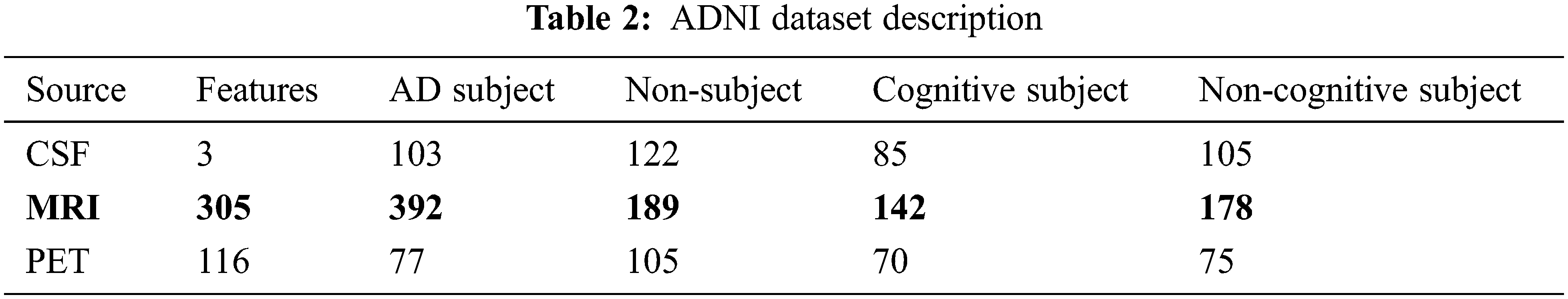
This work uses Alzheimer’s disease Neuroimaging Initiative (ADNI) data composed of 819 samples with 192 AD, 398 MCI and 229 cognitively normal and enrolled based on standard functional and cognitive measures with clinical trials. The target of the construction of the dataset is to measure longitudinal and cross-sectional efforts with normal controls, subjects with mild AD and MCI to facilitate the evaluation of the chemical biomarkers and neuroimaging measures. The samples with MCI are significantly more impaired than the cognitive subjects (standard); however not impaired as AD subjects. Non-memory cognitive measures are impaired minimally with MCI, showing the progression of MCI to dementia. Roughly 50% of MCI subjects are under anti-dementia therapies. There is minimal movement on the AD evaluation scale-cognitive sub-scale for normal control subjects, slight subject movement of MCC with 1.1 and modest variations with AD of 4.3. ADNI is recruited successfully with typical issues, mild cognitive impairment, and AD with baseline characteristics. Table 2 depicts the dataset description.

3.2 Normalization for Pre-Processing

It is the most general approach used for performing pre-processing. It converts the image values into a specific range, i.e., 0 and 1. The normalization approaches considered here are z-score normalization and zero means. It is expressed as in Eq. (1):

Xi′=Xi−mean (X)SD (X) (1)

Here, Xi′ is normalized data; mean (X) specifies the mean value, and SD (X) specifies the standard deviation of input X. The SD is mathematically expressed as in Eq. (2):

σ=1N−1∑i=1N⁡(Xi−mean (X))2 (2)

Here, σ specifies the standard deviation for the provided input values. Along with this, image resizing is also done.

3.3 3D-CNN Model

Before executing the ideas of 3D-CNN, some pre-processing steps like oversampling [15], undersampling [15,16] and data augmentation [17] can be adopted to handle the data imbalance in the anticipated model. Generally, standard CNN performs feature reduction from input to final classification layers. It is followed when the CNN input image is in 3D form, i.e., 3D-MRI image attained from (the ADNI dataset). The inbuilt function in KERAS reads the input, and it is resized from the original 256∗256∗256 to 64∗64∗64 . In a CNN, each layer has two parameters: weights and biases. The total number of parameters is same as the sum of all weights and biases. Multiple downsampling is performed with the max-pool operation for all convolutional layers. Here, dropouts are used to reduce the over-fitting issues and yield Fully-Connected Layers to give the final output class, and it is depicted as the input to the softmax layer. The adoption of Fully connected Layer (FCL) is done to perform the target domain, and it is generally known as fine-tuning. It is considered the essential step for transfer learning with pre-trained networks. It is merged with the large number filters where the weights are kept random (random weights) and updated with back-propagation training. The intermediate layer pretends to identify the activated image parts, while the final layers learn about the discriminative features (pattern and shape) between the target regions. When the training reaches convergence, then it represents that there is no further weight change and training accuracy triggers to the maximum value, thereby terminating the training process. An Activation Function decides whether a neuron should be activated or not, i.e., it determines whether the neuron’s input is essential or not during prediction. Consequently, the proposed CNN model (refer to Fig. 1) is trained and acts as a generic feature extractor like of conventional way of generating the features. The features developed are considered the discriminative features, and it is used for differentiating the classes. Here, 3D filters pretend to give 4D outputs in every connected layer, i.e., 3D feature map/filter. Convoluting the features with the provided filters predicts the occurrence of the features over the image. The filters are equal to 64, 128 and 256. This generic nature of the CNN model is depicted as the baseline for automatic feature extraction and assists computer-aided systems. It is highly complex to predict the features earned by CNN without a training process. Thus, it is a challenging task to examine the features. The network model is composed of millions of parameters, and it is difficult to evaluate the final converged values of every filter devoid of training. Therefore, the features learned have to be analyzed whenever the CNN is introduced. The CNN is loaded with the weighted filter once the model is trained, used for further prediction with the testing images. It is convoluted over every layer to acquire various outcomes for diverse MRIs. Consider, MRI has a 64∗64∗64 matrix specified by I(xi)(yi)(zi) where i=1 to 64. Thus, it results in 144 grey-scale values, determined as the numerical specification for 3D images [18–29].

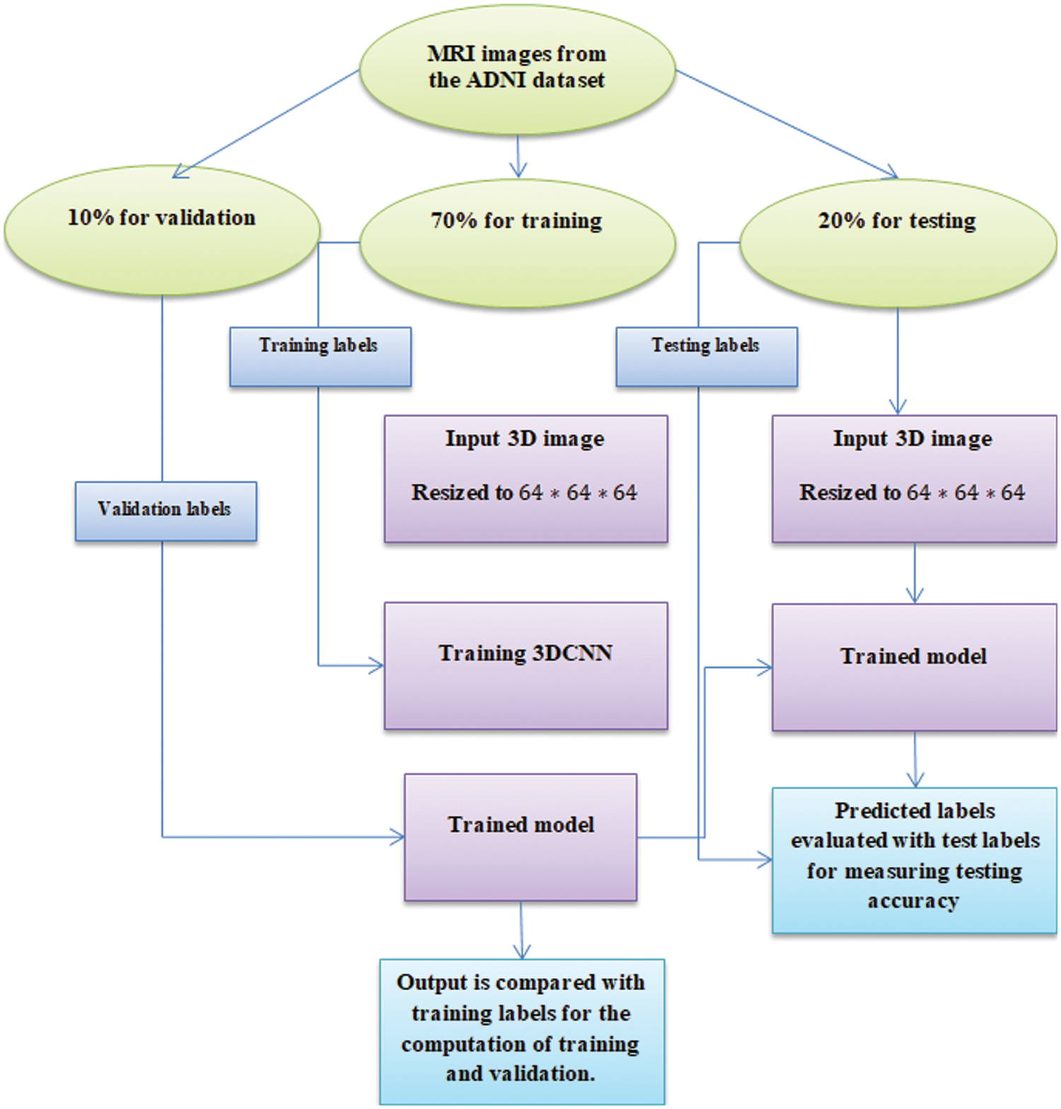
Figure 1: Experimentation workflow

As this research is based on 3D, these values are voxel and not the pixel. Every voxel specifies a 3D value with coordinates (x, y, z) . Here, MRI is represented in the form of a cube. Therefore, every voxel is allocated with three diverse coordinates mathematically for every representation and used the vector notation of v=[Ixiyizi] to make this process so simple and easy. The first convolution over the initial layer is expressed in Eq. (1), where initial bias and weights are represented as b11 and wN,11 , and the importance of convolution kernel over Nth filter with initialization algorithm. Here, ⊙ it specifies element-wise multiplication. The flow is mathematically expressed as in Eq. (3):

[x11,  x21,  x31, …, x641]=[b11,  b21,  b31, …, b641]+[v1,  v2,  v3, …, v9]⊙[(w1,1,1,  w1,22, …, w1,91)] (3)

The convolution operation window keeps moving based on the stride size. The above Eq. (3) is rewritten to reduce the mathematical expression in a shorter form. The nodes of the 3D convolution filter are mathematically expressed as in Eq. (4):

xkl=bkl+∑i=1Nl−1⁡conv3 (wikl−1,  sil−1] (4)

Here, conv3 is a regular 3D convolution devoid of any zero paddings over the boundaries. Eq. (2), xkl is considered an input, bkl is kth neuron bias over the layer ′l′. Then, sil−1 is the ith neuron output at layer l−1 towards kth neuron over layer l. conv3 , which specifies element-wise multiplication over [3*3*3] kernel size. The input sil−1 is supplied as a 3∗3∗3 matrix of image voxel value (normalized) and performed by the same sized window for the initial convolution layer. Fig. 2 shows the blocks of the 3D-CNN model. While representing it in the form of discrete or matrix, N− dimensional convolution in discrete form and variables AquadB are expressed as in Eq. (5):

C(j1,  j2, …, jN)=∑k1⁡…∑kN⁡A (k1,  k2, …, kN)B (j1−k1,  j2−k2,   jN−kN)=convN (A, B) (5)

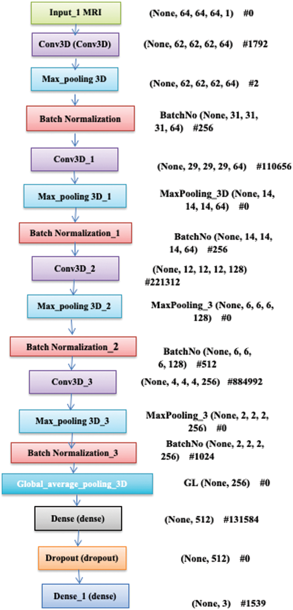
Figure 2: Blocks of 3D-CNN model

For all k1 which runs on values and provides legal sub-scripts for the provided variables A & B. Therefore, 3D convolution runs are provided. The provided network layer convolves the input by eliminating the filters (horizontal and vertical) filters. However, it evaluates the weighted dot products and input, which subsequently adds to the bias term. When the filtering is done along with the input, it utilizes a similar weighted set and bias for performing convolution. Therefore, it forms feature mapping. With stochastic Gradient descent, the weighted filters are iteratively optimized, and it is updated based on the provided Eqs. (6) and (7):

Wlt+1=Wlt+Vlt+1 (6)

Here, Walt specifies the lth convolution layer weights for every lth iteration, and E specifies the cost function by back-propagation updation for reducing the cost function over the mini-batch with ′N′ size. It is expressed as in Eq. (7):

Vl(t+1)=m. Vlt− γlt . αldEdWl (7)

Here, ∝l specifies the lth layer-based learning rate, ′m′ is momentum based on prior weight updation over the current iteration, γ is defined as scheduling rate, which reduces the learning rate for every epoch completion. When αl=0 and it relies on the value 1. All the layers from 1 to l are not updated with weight. Therefore, the weights are moved to the final trained model. The parameter tuning is achieved with Eq. (8):

Totalerror(E)=E(y1L, …, yNL)=∑i=1NL⁡(yiL−ti)2 (8)

Here, the error is considered Mean Square Error by accumulating the MSE value of the samples derived, i.e., trained data from predicted data. Here, L specifies the final layer output and BP is performed for weight updation for all parameters over Eq. (9):

∂E∂wikl=∂E∂xkl+1. ∂xkl+1∂wikl=∂E∂xkl+1. yil (9)

Here, xkl+1 is the kth filter output which is the number of lth layer filters, and the weight of the previous layers l+1  provides yil layer where the bias is updated based on Eq. (10):

∂E∂bkl=∂E∂xkl. ∂xkl∂wkl=∂E∂xkl (10)

Based on Eq. (10), the result is provided as the entire length with 1 to l+1 . Therefore, it is added for N filters over the l+1  layers to attain y in the lth layer, and it is expressed as in Eq. (11):

∂E∂ykl=∑i−1Nl+1∂E∂xil+1. ∂xil+1∂ykl (11)

During the training process, the gradient error needs to be BP via the transformation and evaluate the gradients based on the parameters like batch normalization transformation. The initial layers are tested, i.e., convolutional-batch normalization, max-pooling and ReLU are defined based on the optimal layers with 64∗64∗64 input (3D scan). The blocks are executed based on the provided layers L1 to 4. The final feature size with convolution [2 2 2] is provided for all 64 filters. It shows that the filter kernels possess two pixels for all filters. Therefore, this work does not consider more than five convolution layers. The training and validation are provided to project how the proposed 3D-CNN influences the training process and assists in having a better understanding of the convergence process for all CNN. The MRI for all domains is passed to better understand the feature extraction from the provided convolutional layers, and every layer is monitored. The observations help predict the difference among the patterns, intensities, lines and edges [30,31]. The layers are visualized for the entire testing set and, therefore, help segregate the features from the provided framework in a superior manner. At last, the outcomes from the various hyper-parameter setting are provided [32–37].

The filter size depicts the scanning window during the convolution process, and two strides increment window size for all consecutive layers. Therefore, the extracted features are sequentially at a lower, intermediate and higher level. Here, the low-level features are removed from filter window 3∗3∗3 and maximum-pooling by 2∗2∗2 windows with a stride of the convolutional layers. The filter size increases based on the step size; however, the filters of every layer are provided as 64. It is done to preserve the channel size for the given input 64∗64∗64 . Thus, the variations are captured more straightforwardly. When the layer moves more profoundly, the features are accumulated by increasing the window size of all layers. The maximum-pooling strides are also increased to diminish the feature redundancy. The kernel size is uniform, with 3∗3∗3 for all convolutional layers. The outcomes after the training, testing and validation are discussed below. The layer details are shown in Table 3.

4  Numerical Results and Discussion

Here, four diverse performance metrics are utilized for evaluation purpose and they are: accuracy, recall, precision, and F1-score. In the equation given below, True Negative (TN), True Positive (TP), False Negative (FN) and False Positive (FP) are used for evaluation, and it is expressed as in Eqs. (12)–(15):

Accuracy=TP+TNTP+FP+FN+TN (12)

Precision=TPTP+FP (13)

Recall=TPTP+FN (14)

f1−score=2TP2TP+FP+FN (15)

Here, the ADNI dataset is used where 800 samples are adopted for training, and 200 samples are adopted for testing with a partitioning ratio of 70:30, i.e., 70 for training, 20 for testing and 10 for validation.

Table 4 depicts the anticipated 3D-CNN performance with existing LSTM-RNN, SAE-DNN, D-CNN, and 2D-CNN models. Here, metrics like accuracy, precision, recall, and F1-score are evaluated and compared among these models. The prediction accuracy of 3D-CNN is 89.47% which is 11.47%, 12.47%, and 13.47% higher than LSTM-RNN, SAE-DNN, D-CNN and 2D-CNN, as depicted in Fig. 5. The 3D-CNN precision is 86.66% which is 18.66%, 13.66%, and 2.667% higher than LSTM-RNN, SAE-DNN, D-CNN and 2D-CNN. The recall of 3D-CNN is 89.47% which is 11.47%, 12.47%, and 13.47% higher than LSTM-RNN, SAE-DNN, D-CNN and 2D-CNN. The F1-score of 3D-CNN is 90.41% which is 18.41%, 15.41%, and 8.41% higher than LSTM-RNN, SAE-DNN, D-CNN and 2D-CNN.

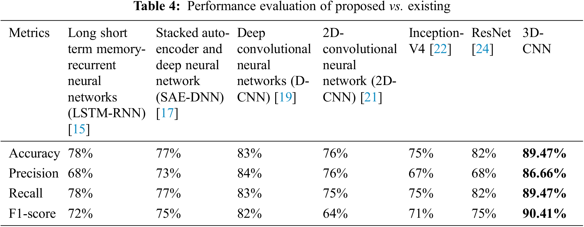
Table 4 depicts the anticipated 3D-CNN performance with existing Inception-V4, ResNet, and D-CNN models. Here, metrics like accuracy, precision, recall, and F1-score are evaluated and compared among these models. The prediction accuracy of 3D-CNN is 89.47% which is 14.47%, 7.47%, and 6.47% higher than Inception-V4, ResNet, and D-CNN. The precision of 3D-CNN is 86.66% which is 19.66%, 18.66%, and 2.66% higher than Inception-V4, ResNet, and D-CNN. The recall of 3D-CNN is 89.47% which is 14.47%, 7.47%, and 6.47% higher than Inception-V4, ResNet, and D-CNN. The F1-score of 3D-CNN is 90.41% which is 19.41%, 15.41%, and 8.41% higher than Inception-V4, ResNet, and D-CNN, respectively. Figs. 3–6 depicts the overall comparison of the anticipated model with the existing approaches. Fig. 7 shows the training and validation accuracy, and Fig. 8 shows the training and validation loss. Finally, Fig. 9 shows the prediction outcome of the anticipated model.

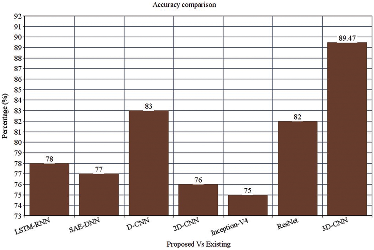
Figure 3: Accuracy comparison

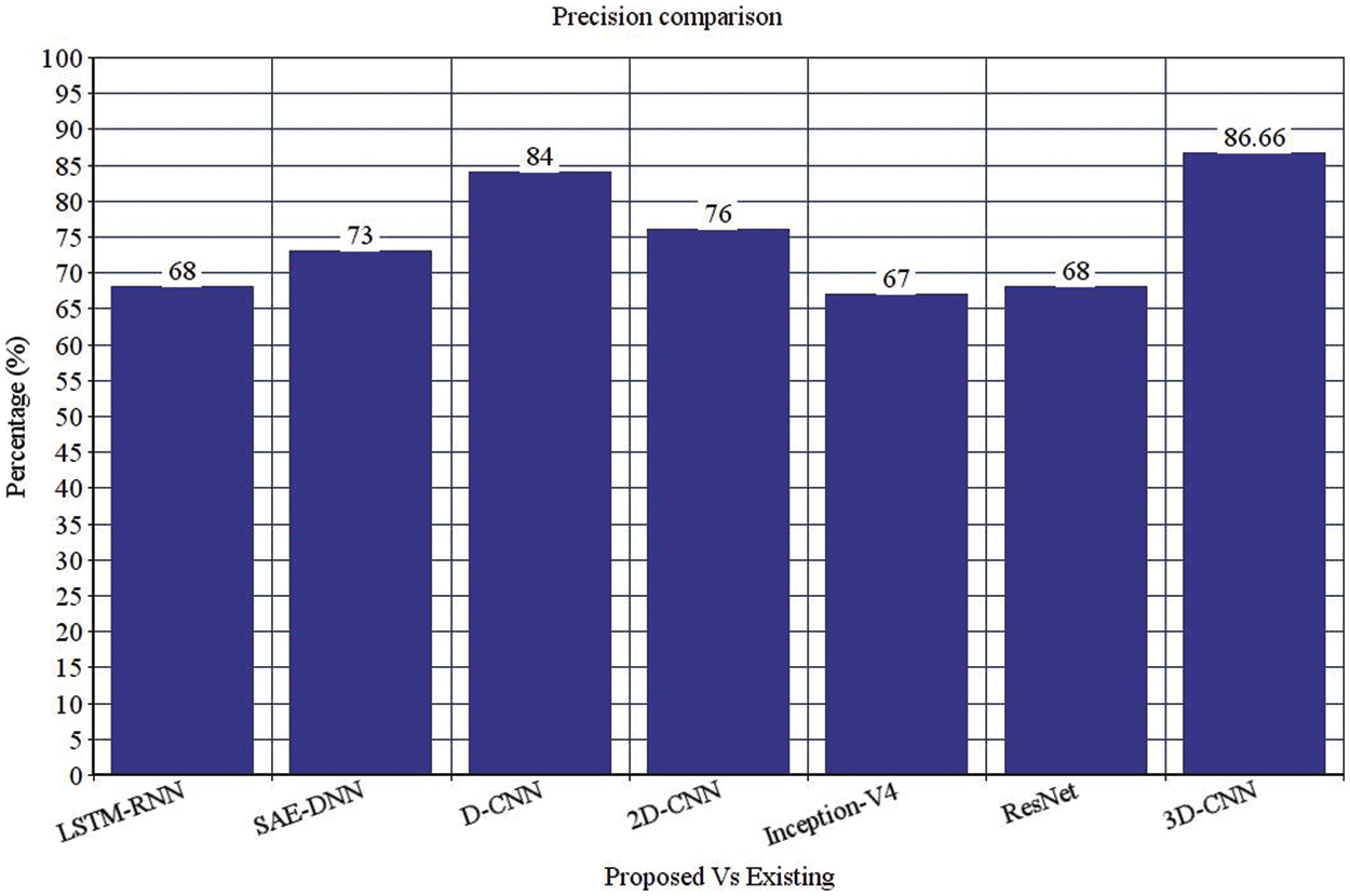
Figure 4: Precision comparison

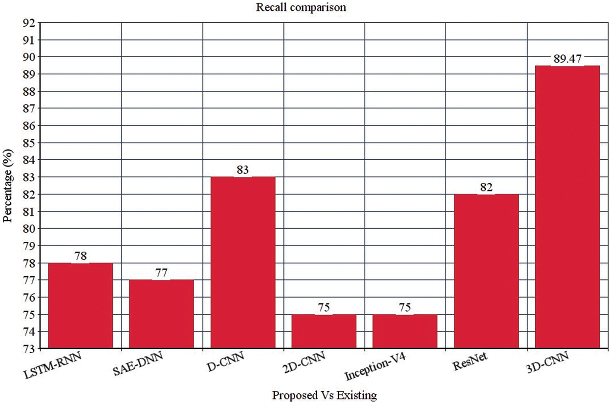
Figure 5: Recall comparison

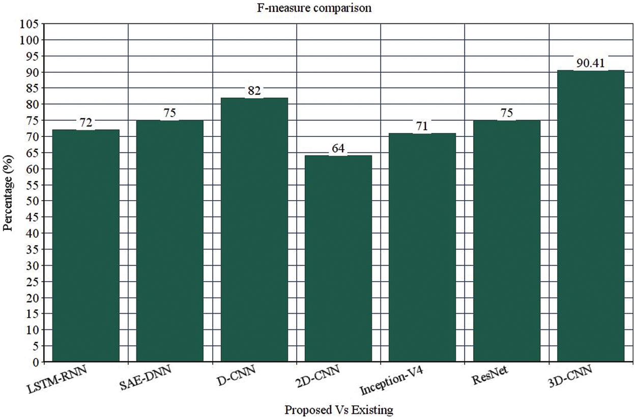
Figure 6: F-measure comparison

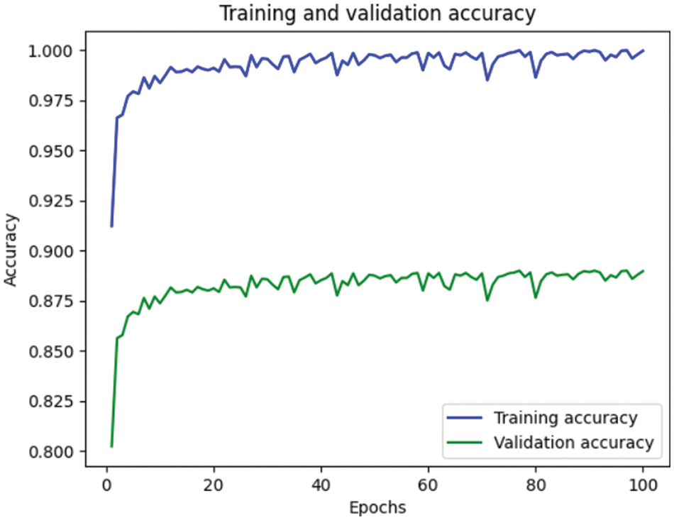
Figure 7: Representation of training and validation accuracy

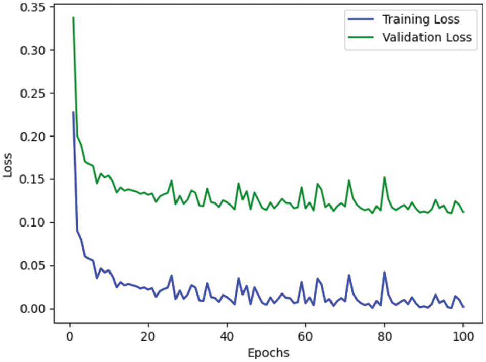
Figure 8: Representation of training and validation loss

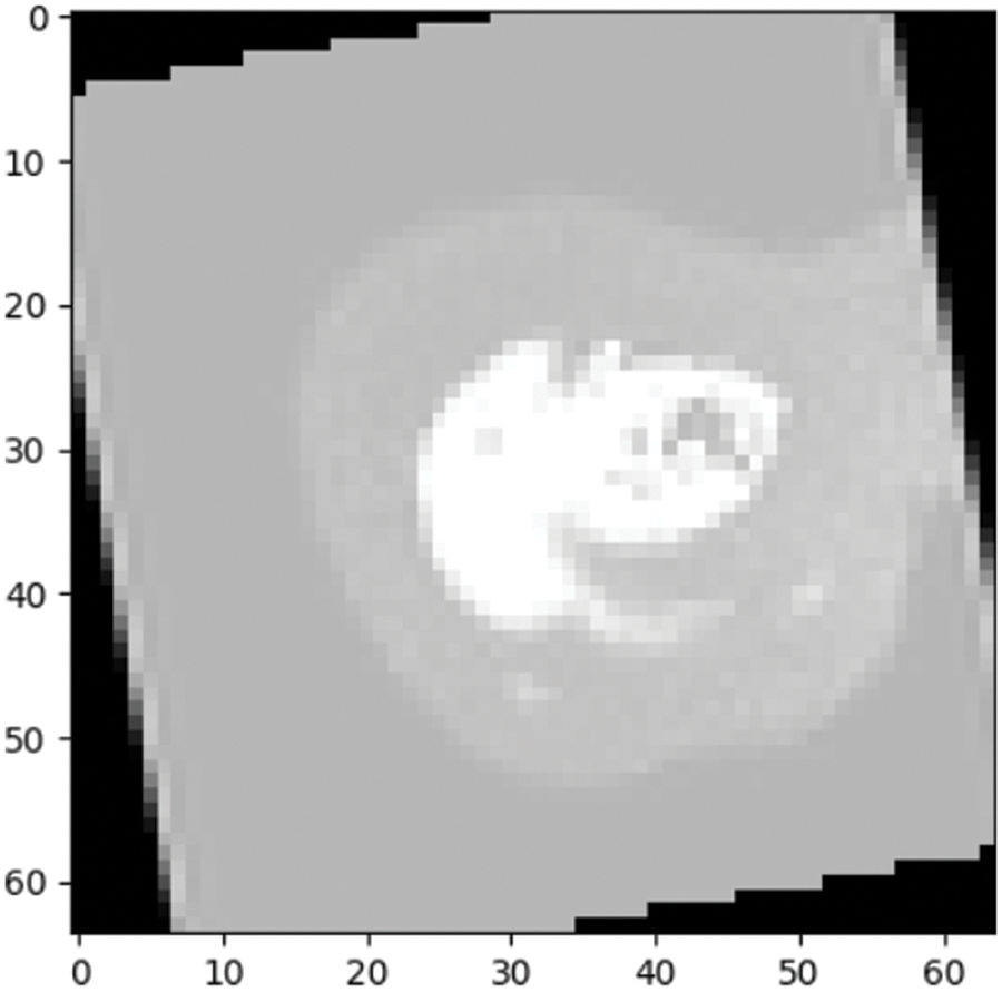
Figure 9: Prediction outcome

From the analysis of the past few decades, the hybridization approach integrates the conventional learning approaches for diagnostic prediction with DL approaches for extracting features and yields superior performance. Fig. 10 depicts the confusion matrix of the anticipated model. Generally, DL needs considerable data to attain desired performance levels and prediction accuracy. It is considered an excellent alternative to deal with these constraint data. Even though hybrid approaches have achieved relatively superior outcomes, they do not benefit DL, which extracts features automatically from a large amount of neuroimaging data. The most commonly adopted DL approaches in computer vision studies is CNN, which specializes in removing images’ characteristics. Currently, 3D-CNN models are proposed in this work and show superior performance for AD classification.

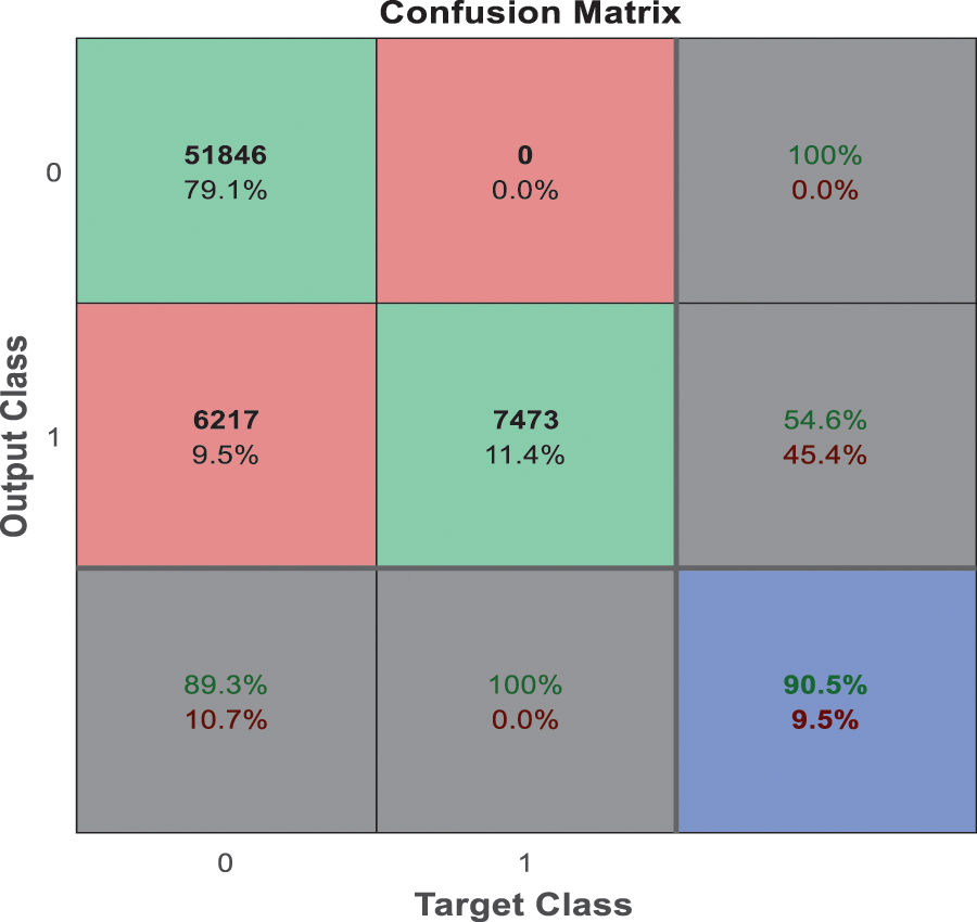
Figure 10: Confusion matrix

5  Conclusion

This work provides a productive approach for AD prediction using MRI brain image analysis. Various existing research works concentrate on performing binary and multi-class classification; however, the enhancement of prediction accuracy is highly solicited. The anticipated 3D-network architecture is exceptionally beneficial for predicting AD in its earlier stage. Based on this research progression, the expected 3D-CNN model is tested over the AD dataset; it is applied to other research in the medical field. The proposed 3D-CNN model gives a prediction accuracy of 89.47%, precision of 86.66%, recall of 89.47% and F1-score of 90.41%, which is higher than LSTM-RNN, SAE-DNN, D-CNN, 2D-CNN, AD-Net, ResNet, and Inception-V4. Here, the prediction and validation accuracy intends to eliminate the over-fitting issues encountered in the previous research works. The proposed 3D-CNN model provides promising outcomes which may be further improved in the future. However, the primary research constraint is the acquisition of dataset images. In the future, the anticipated 3D-CNN model needs to be tested over various other AD datasets and other-brain related disease diagnoses. The prediction of AD using DL still evolves to attain superior prediction accuracy and transparency. The research on AD diagnostic classification is shifting towards deep learning instead of other prediction methods. In future, some techniques must be modelled to merge diverse data formats in the deep learning network model.

Funding Statement: The authors received no specific funding for this study.

Conflicts of Interest: The authors declare that they have no conflicts of interest to report regarding the present study.

References

    1. M. J. Prince, “Alzheimer’s disease facts and figures,” Alzheimer’s Dementia, vol. 14, no. 3, pp. 367–429, 2018. [Google Scholar]

    2. Y. Bengio, A. Courville and P. Vincent, “Representation learning: A review and new perspectives,” IEEE Transactions on Pattern Analysis and Machine Intelligence, vol. 35, no. 8, pp. 1798–1828, 2013. [Google Scholar]

    3. Y. L. Boureau, J. Ponce and Y. Lecun, “A theoretical analysis of feature pooling in visual recognition,” in Proc. 27th Int. Conf. on Machine Learning (ICML-10), Haifa, Israel, pp. 111–118, 2010. [Google Scholar]

    4. D. Cheng and M. Liu, “CNN’s based multi-modality classification for AD diagnosis,” in 10th Int. Congress on Image and Signal Processing, Biomedical Engineering and Informatics (CISP-BMEI), Shanghai, China, pp. 1–5, 2017. [Google Scholar]

    5. H. Choi and K. H. Jin, “Predicting cognitive decline with deep learning of brain metabolism and amyloid imaging,” Behavioural Brain Research, vol. 344, no. 2, pp. 103–109, 2018. [Google Scholar]

    6. D. Cregan, U. Meier and J. Schmidhuber, “Multi-column deep neural networks for image classification,” in IEEE Conf. on Computer Vision and Pattern Recognition, Rhode Island, United States, pp. 3642–3649, 2012. [Google Scholar]

    7. C. Farabet, C. Couprie, L. Najman and Y. Lecun, “Learning hierarchical features for scene labelling,” IEEE Transactions on Pattern Analysis and Machine Intelligence, vol. 35, no. 8, pp. 1915–1929, 2013. [Google Scholar]

    8. K. Fukushima, “Neocognitron: A self-organizing neural network model for a mechanism of pattern recognition unaffected by shift in position,” Biological Cybernetics, vol. 36, no. 7, pp. 193–202, 1980. [Google Scholar]

    9. X. Glorot, A. Bordes and Y. Bengio, “Deep sparse rectifier neural networks,” in Proc. of the Fourteenth Int. Conf. on Artificial Intelligence and Statistics, Fort Lauderdale, Florida, United States, pp. 315–323, 2011. [Google Scholar]

  10. V. Gulshan, L. Peng, M. Coram, M. C. Stumpe, D. Wu et al., “Development and validation of a deep learning algorithm for detection of diabetic retinopathy in retinal fundus photographs,” JAMA, vol. 316, no. 22, pp. 2402–2410, 2016. [Google Scholar]

  11. S. Liu, S. Liu, W. Cai, S. Pujol, R. Kikinis et al., “Early diagnosis of Alzheimer’s disease with deep learning,” in IEEE 11th Int. Symp. on Biomedical Imaging (ISBI), Beijing, China, pp. 1015–1018, 2014. [Google Scholar]

  12. D. Lu, K. Popuri, G. W. Ding, R. Balachandar and M. F. Beg, “Multi-modal and multiscale deep neural networks for the early diagnosis of Alzheimer’s disease using structural MR and FDG-PET images,” Scientific Reports, vol. 8, no. 1, pp. 1–13, 2018. [Google Scholar]

  13. H. I. Suk, S. W. Lee and D. Shen, “Latent feature representation with stacked auto-encoder for AD/MCI diagnosis,” Brain Structure and Function, vol. 220, no. 2, pp. 841–859, 2015. [Google Scholar]

  14. D. P. Veitch, M. W. Weiner, P. S. Aisen, L. A. Beckett, N. J. Cairns et al., “Understanding disease progression and improving Alzheimer’s disease clinical trials: Recent highlights from the Alzheimer’s disease neuroimaging initiative,” Alzheimer’s & Dementia, vol. 15, no. 1, pp. 106–152, 2019. [Google Scholar]

  15. M. Bucholc, X. Ding, H. Wang, D. H. Glass, H. Wang et al., “A practical computerized decision support system for predicting an individual’s severity of Alzheimer’s disease,” Expert Systems with Applications, vol. 130, no. 2, pp. 157–171, 2019. [Google Scholar]

  16. D. Zhang and D. Shen, “Multi-modal multitask learning for joint prediction of multiple regression and classification variables in Alzheimer’s disease,” NeuroImage, vol. 59, no. 2, pp. 895–907, 2012. [Google Scholar]

  17. E. Moradi, A. Pepe, C. Gaser, H. Huttunen and J. Tohka, “Machine learning framework for early MRI-based Alzheimer’s conversion prediction in MCI subjects,” NeuroImage, vol. 104, no. 5, pp. 398–412, 2015. [Google Scholar]

  18. X. Zhao, Y. Wu, D. L. Lee and W. Cui, “iForest: Interpreting random forests via visual analytics,” IEEE Transactions on Visualization and Computer Graphics, vol. 25, no. 1, pp. 407–416, 2018. [Google Scholar]

  19. J. Ramírez, J. M. Górriz, A. Ortiz, F. J. Martínez-Murcia, F. Segovia et al., “Ensemble random forests one vs rest classifiers for MCI and AD prediction using ANOVA cortical and subcortical feature selection and partial least squares,” Journal of Neuroscience Methods, vol. 302, no. 1, pp. 47–57, 2018. [Google Scholar]

  20. S. El-Sappagh, T. Ahmed, S. M. R. Islam and K. S. Kwak, “Multimodal multitask deep learning model for Alzheimer’s disease progression detection based on time series data,” Neurocomputing, vol. 412, no. 2, pp. 197–215, 2020. [Google Scholar]

  21. G. McKhann, “Clinical diagnosis of Alzheimer’s disease: Report of the NINCDS-ADRDA work group under the auspices of department of health and human services task force on Alzheimer’s disease,” Neurology, vol. 34, no. 1, pp. 939, 2004. [Google Scholar]

  22. S. Afzal, M. Maqsood, F. Nazir, U. Khan, F. Aadil et al., “A data augmentation-based framework to handle class imbalance problem Alzheimer’s stage detection,” IEEE Access, vol. 7, no. 2, pp. 115528–115539, 2019. [Google Scholar]

  23. T. Altaf, S. M. Anwar, N. Gul, M. N. Majeed and M. Majid, “Multi-class Alzheimer’s disease classification using the image and clinical features,” Biomedical Signal Processing and Control, vol. 43, no. 4, pp. 64–74, 2018. [Google Scholar]

  24. S. Manimurugan, “Classification of Alzheimer’s disease from MRI images using CNN based pre-trained VGG-19 model,” Journal of Computational Science and Intelligent Technologies, vol. 1, no. 2, pp. 34–41, 2020. [Google Scholar]

  25. X. W. Gao, R. Hui and Z. Tian, “Classification of CT brain images based on deep learning networks,” Computer Methods and Programs in Biomedicine, vol. 138, no. 3, pp. 49–56, 2017. [Google Scholar]

  26. M. R. Brier, J. B. Thomas, A. Z. Snyder, T. L. Benzinger, D. Zhang et al., “Loss of intranetwork and internetwork resting-state functional connections with Alzheimer’s disease progression,” Journal of Neuroscience, vol. 32, no. 26, pp. 8890–8899, 2012. [Google Scholar]

  27. D. D. Cox and R. L. Savoy, “Functional magnetic resonance imaging (fMRI) “brain reading”: Detecting and classifying distributed patterns of fMRI activity in human visual cortex,” Neuroimage, vol. 19, no. 2, pp. 261–270, 2003. [Google Scholar]

  28. R. Sukkar, E. Katz, Y. Zhang, D. Raunig and B. T. Wyman, “Disease progression modelling using hidden Markov models,” in Proc. of Annual Int. Conf. of IEEE Engineering in Medicine and Biology Society (EMBC), San Diego, CA, USA, pp. 2845–2848, 2012. [Google Scholar]

  29. Y. Noh, S. Jeon, J. M. Lee, S. W. Seo, G. H. Kim et al., “Anatomical heterogeneity of Alzheimer disease: Based on the cortical thickness on MRIs,” Neurology, vol. 83, no. 4, pp. 1936–1944, 2014. [Google Scholar]

  30. M. Odusami, R. Maskellunas and R. Damasevicius, “An intelligent system for early recognition of Alzheimer’s disease using neuroimaging,” Sensors, vol. 22, no. 3, pp. 1865–1870, 2022. [Google Scholar]

  31. Y. Wang, X. Liu and C. Yu, “Assisted diagnosis of Alzheimer’s disease based on deep learning and multimodal feature fusion,” Hindawi, vol. 1, no. 2, pp. 75–90, 2021. [Google Scholar]

  32. D. Pan, A. Zeng, L. Jia, Y. Hunag, T. Frizzell et al., “Early detection of Alzheimer’s disease using magnetic resonance imaging: A novel approach combining convolutional neural networks and ensemble learning,” Neuroscience, vol. 13, no. 259, pp. 1–19, 2020. [Google Scholar]

  33. M. B. Sudhan, M. Sinthuja, S. P. Raja, J. Amutharaj, G. C. P. Latha et al., “Segmentation and classification of glaucoma using U-Net with deep learning model,” Journal of Healthcare Engineering, vol. 2022, no. 1601354, pp. 1–10, 2022. [Google Scholar]

  34. S. Sridhar, J. Amutharaj, V. Prajoona, B. Arthi, S. Ramkumar et al.,“A torn ACL mapping in knee MRI images using deep convolution neural network with inception-v3,” Journal of Healthcare Engineering, vol. 2022, no. 7872500, pp. 1–9, 2022. [Google Scholar]

  35. S. Rinesh, K. Maheswari, B. Arthi, P. Sherubha, A. Vijay et al., “Investigations on brain tumor classification using hybrid machine learning algorithms,” Journal of Healthcare Engineering, vol. 2022, no. 2761847, pp. 1–9, 2022. [Google Scholar]

  36. T. Rajendran, K. P. Sridhar and S. Manimurugan,“Recent innovations in soft computing applications,” Current Signal Transduction Therapy, vol. 14, no. 2, pp. 129–130, 2019. [Google Scholar]

  37. T. Rajendran, K. P. Sridhar, S. Manimurugan and S. Deepa, “Advanced algorithms for medical image processing,” The Open Biomedical Engineering Journal, vol. 13, no. 1, pp. 102, 2019. [Google Scholar]