
 Submit a Paper
 Propose a Special lssue
 Open Access
ARTICLE

Quantum Computing Based Neural Networks for Anomaly Classification in Real-Time Surveillance Videos
1 Department of Computer Science Engineering, Jairupaa College of Engineering Thottiapalayam, Tirupur District, 641604, Tamilnadu, India
2 Department of Electronics and Communications Engineering, Dhanalakshmi College of Engineering, Chennai, 600015, Tamilnadu, India
* Corresponding Author: MD. Yasar Arafath. Email:
Computer Systems Science and Engineering 2023, 46(2), 2489-2508. https://doi.org/10.32604/csse.2023.035732
Received 01 September 2022; Accepted 08 December 2022; Issue published 09 February 2023
 View Full Text
 Download PDF
Abstract
For intelligent surveillance videos, anomaly detection is extremely important. Deep learning algorithms have been popular for evaluating real-time surveillance recordings, like traffic accidents, and criminal or unlawful incidents such as suicide attempts. Nevertheless, Deep learning methods for classification, like convolutional neural networks, necessitate a lot of computing power. Quantum computing is a branch of technology that solves abnormal and complex problems using quantum mechanics. As a result, the focus of this research is on developing a hybrid quantum computing model which is based on deep learning. This research develops a Quantum Computing-based Convolutional Neural Network (QC-CNN) to extract features and classify anomalies from surveillance footage. A Quantum-based Circuit, such as the real amplitude circuit, is utilized to improve the performance of the model. As far as my research, this is the first work to employ quantum deep learning techniques to classify anomalous events in video surveillance applications. There are 13 anomalies classified from the UCF-crime dataset. Based on experimental results, the proposed model is capable of efficiently classifying data concerning confusion matrix, Receiver Operating Characteristic (ROC), accuracy, Area Under Curve (AUC), precision, recall as well as F1-score. The proposed QC-CNN has attained the best accuracy of 95.65 percent which is 5.37% greater when compared to other existing models. To measure the efficiency of the proposed work, QC-CNN is also evaluated with classical and quantum models.Keywords
Surveillance is quickly gaining popularity due to technological advancement that may be utilized to safeguard life safety as well as break through security barriers. Closed-Circuit Television (CCTV) cameras were broadly utilized for monitoring and security events, as well as supplying proof to the surveillance system [1].
These cameras continually create massive amounts of video data, necessitating manual monitoring attempts which are both time-consuming and inaccurate, necessitating the use of automated monitoring approaches. Because of the limited effectiveness of surveillance using humans, law enforcement authorities had a difficult time catching or averting unusual situations. A computer vision-based system that can successfully identify normal or anomalous occurrences without human intervention is needed to identify anomalous activity. This automated system not only aids in monitoring, but it also decreases the amount of human labor necessary to sustain 24-hour manual observation [2]. Anomalous behavior identification is the process of detecting patterns as well as occurrences that differ from the usual [3].
Researchers have developed a few new strategies for detecting anomalies in surveillance footage [4–12]. These studies identify anomalies in surveillance recordings of populated spaces such as retail malls and public areas. They primarily concentrate on binary categorization, such as aggressive or disaster, and thus provide a partial answer for application in real-world circumstances. In real-life circumstances, the efficiency of the algorithms was significantly inferior because the various and dense form of monitoring data renders it difficult to identify all probable abnormal occurrences.
The majority of the above strategies struggle from a high false alarm rate. Moreover, while these strategies function very effectively on simple datasets, their efficiency is restricted when dealing with real-life events. Also, the computation process to detect and classify multiple anomaly types is higher. The accuracy of anomaly detection should be further improved.
Quantum computing becomes a potential subject that may be able to assist to solve this issue through drastically new structures. As a result, research and development of new deep learning algorithms relying on quantum computers become critical to stay up with possible AI achievements.
Quantum computing could be a whole new computing model which uses quantum physics rather than conventional physics. Rather than traditional bits, quantum computing employs quantum bits, also qubits, which work with the superposition as well as uncertainty inherent in quantum physics [13]. Researchers investigated and presented the viability of expanding machine learning systems into the quantum domain to attain considerably enhanced results. Previous research has shown that quantum machine learning techniques possess a high potential for solving traditional tasks [14].
Some works used quantum machine learning for image classification tasks [14–17]. Inspired by this, an anomaly event detection and classification model are proposed for detecting anomalous events in surveillance videos. To the best of our understanding, this is the first work to use quantum deep learning for anomalous event classification.
The key contributions can be summarized as follows.
• To propose a Quantum deep learning-based model named Quantum Computing based Convolutional Neural Network (QC-CNN) for anomaly detection and classification in surveillance videos. To obtain better performance through the quantum-based circuit, such as an absolute amplitude circuit.
• The results of testing the proposed models using the benchmark dataset UCF-Crime show better performances than existing works. Concerning accuracy, ROC, AUC, precision, recall, and F1-score, the proposed QC-CNN surpasses existing techniques.
The rest of this work is organized as follows. Section 2 summarises the associated research on anomalous behavior recognition techniques. Section 3 introduces the proposed abnormal event detection approach, as well as the Quantum Computing-based deep learning approach. Section 4 contains the experimental outcomes. Section 5 ends with the conclusion.
Deep learning using a homomorphic encryption technique has been introduced in [18] to secure data privacy whenever customers utilize the cloud-based deep learning approach. However, the complexity is high when the depth of the networks is increased. The detection rate was tested in [19] by feeding adversarial data into the Autoencoder as well as Convolution Neural Network (CNN). But other parameters to verify the model were not discussed.
A new anomaly detection technique is proposed in [20] to find anomalies in surveillance videos. CNN and two prominent customized approaches were used for feature extraction from videos. This method fails to recognize some anomalous frames due to their similarity to regular ones.
In [21], a new two-stream-based convolutional network method for identifying anomalies from surveillance footage was suggested. Nevertheless, considering new inputs, the suggested anomalous event detection approach requires development.
To detect unusual occurrences in the surveillance camera, a novel structure combining ResNet50 and ConvLSTM was proposed in [22]. But, the accuracy is not improved by the designed method.
The authors of [23] presented a Quantum Generative Adversarial Network (QGAN) design for a cloud-based human-centered approach. The synthetic dataset is utilized in this work for traditional data categorization problems. The authors of [24] suggested a Hybrid classical-quantum Autoencoder (HAE) model with four datasets for monitoring gas power stations. The anomaly is detected and the performance is evaluated here.
For medical image classification, two models, Quantum orthogonal neural Networks (QONN) and Quantum-assisted Neural Networks (QANN) were proposed in [25]. All of the existing methods are based on quantum machine learning and serve different purposes. There are no existing quantum machine learning models in video surveillance applications, as far as we know.
Variational quantum circuits with deep reinforcement learning were researched by Chen et al. (2020) [26]. To describe variational quantum circuits, they rebuilt classical deep reinforcement learning methods like experience replay as well as target network. Also, they adopted a quantum information encoding approach to reduce the number of model parameters when compared to traditional neural networks. Yano et al. (2021) [27] suggested a quantum classifier based on Quantum Random-Access Coding (QRAC) for a discrete-featured dataset. The system’s major benefit is that it offers a mechanism for encoding an input bitstring to a quantum state with fewer quantum bits.
This section describes the proposed work in detail. Using a Quantum machine learning model, anomalies in real-time surveillance videos are detected and classified. Quantum Computing based Convolutional Neural Network (QC-CNN) is proposed, detailed in the subsections below.
The flow of the proposed work is given in Fig. 1. The very first step involves dividing the dataset to test data and training data according to the input videos in the dataset. The next step is to pre-process the original video, where the video frames are extracted and resized. From the pre-processed training data, the spatiotemporal features are removed, and then anomaly detection and classification are performed. Using the test dataset, the anomaly detection from the video frames is evaluated. 13 real-world anomalies are classified from the surveillance videos.
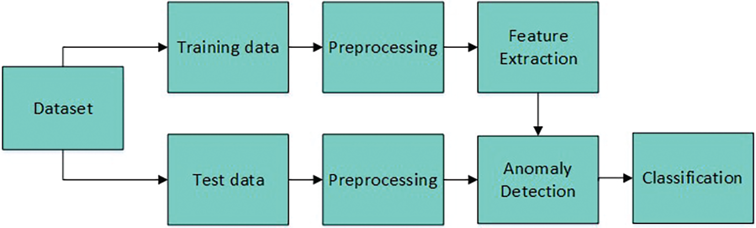
Figure 1: Flow diagram of proposed work
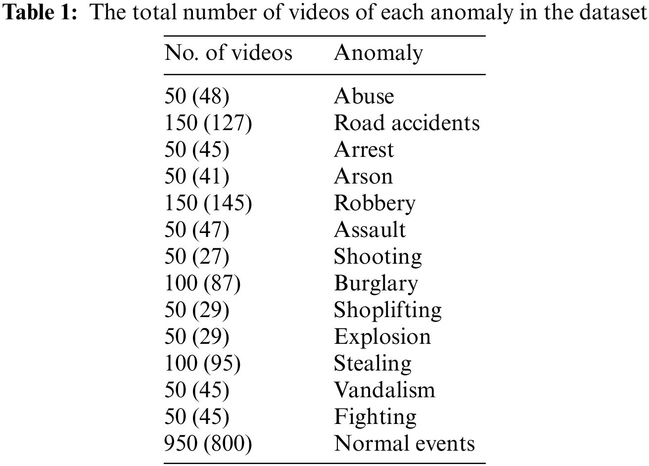
The dataset from which the proposed method was evaluated [28]. It comprises uncut surveillance recordings which include 13 real-life anomalies, involving Explosion, Robbery, Abuse, Shooting, Arson, Shoplifting, Assault, Vandalism, Fighting, and Burglary. These anomalies were chosen because they pose a serious threat to public safety. The dataset is 128 h long, with an average of 7247 frames in 1900 videos.
Training and test data: The dataset is divided into two sections: a training set with 800 normal videos and 810 anomalous videos (described in Table 1). A testing set comprises 150 normal videos and 140 abnormal videos. The 13 anomalies from the videos across various temporal positions are present in both the training and testing sets. In Table 1, the numbers in brackets denote the training set’s number of videos.
It includes extracting frames from a video sequence. Following that, each obtained video frame is resized according to the input size of the model which is utilized in the subsequent steps of feature extraction. To be compatible with the proposed procedure, the UCF-crime dataset is split into many video frames. After that, each video frame size is standardized to 224 × 224 × 64. The pre-processing of an image enables it to be fed into a Classification model. An identical set of procedures were used in the testing phase of this research. The proposed model was tested on videos; therefore, the frames of the videos were looped while testing and all of the frames were treated to the same pre-processing as the training images.
3.4 Basic Notations on Quantum Computing
In quantum computers, qubits [29] seem to be the basic units of data. A physical qubit resides in a state that is a superposition of two others,
The state
Quantum measurement seems to be an irreversible process, where data regarding a one qubit’s state is obtained while superposition gets destroyed. In terms of Hilbert Space,
where
Quantum gates, indicated using the letter Z and it is the fundamental quantum circuits that operate with a finite amount of qubits. It serves as a foundation for quantum circuits in the same way that classical logic gates serve as the foundation for ordinary digital circuits. Quantum gates were known as unitary operators, and it can be denoted as Z
The typical quantum gates utilized here were discussed further below.
1) Hadamard gate, which seems to be a one-qubit gate can be defined as,
This gate provides the superposition principle of two states, particularly plus state, beginning with the single state qubit
2) Rotation gates,
3) CNOT gate, which is a two-qubit gate can be defined as,
Whenever the input consists of the fundamental states
That is, it switches the second qubit (which is the targeted qubit) only when the first qubit (controlled) is
A quantum circuit that is parameterized is generally utilized as a hidden layer to construct a hybrid QNN in the neural network. However, in the case of classical network topologies, realizing a quantum representation of classical data which is high higher dimensional while building the hybrid model is crucial for incorporating the quantum element into the classical design. A basic discussion of how to create a quantum state at this point is provided in this work.
A unitary operator is used to process a feature mapping first. This is given to a group of N|0⟩ quantum nodes as a method for encoding classical data in the new N-qubit space. Before actually applying this to the quantum circuit, a unitary matrix should be traditionally constructed. The previous classical node values at the moment of insertion define its parameters. The previous classical activation can be reflected by the associated amplitude probability for estimating |1⟩ in this process in the quantum state, which is known as data embedding.
The parameterized quantum circuit has been used after the classical encoding process. A parameterized quantum circuit is one in which the rotation angles of every gate are defined with the help of elements in a classical vector (input). The output from a prior layer in the neural network can be gathered and utilized as input for the parameterized circuit. The measured data from the quantum circuit is gathered and given to the next hidden layer. Fig. 2 depicts the configuration between classical and quantum layers as an illustration [29].
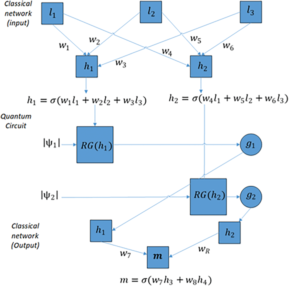
Figure 2: The interface between classical and quantum layers
3.6 Quantum Circuit for Anomaly Detection and Classification
A real amplitude circuit (Quantum circuit) is selected to be used in the proposed QC-CNN [29]. This will give us a better understanding of how the final output is affected by gates and assist in speeding the key computing procedures.
As seen in Fig. 3, every qubit travels via Hadamard gate. Then, experience gate rotation having parameters θ (θ can be obtained from the output of the previous classical node). This procedure can be used for converting classical information into quantum data. The qubits would then be progressively entangled with the use of CNOT gates. The second parameter θ is utilized as “quantum weights” translating toward the subsequent nodes in the classically fully connected layer throughout the validation as well as testing procedure.
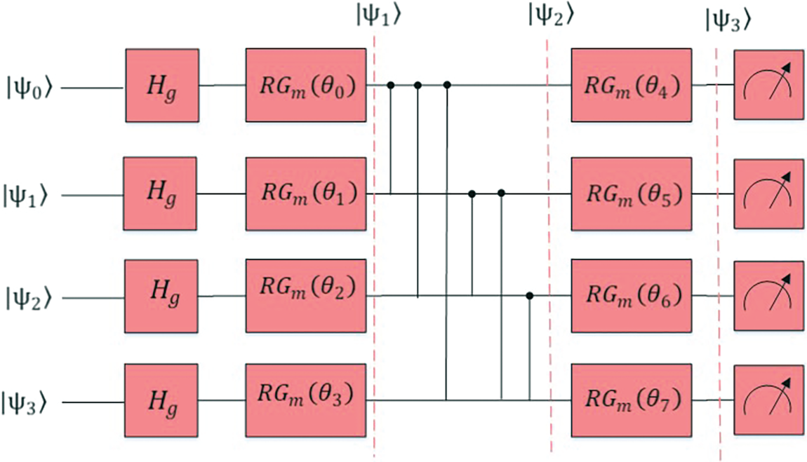
Figure 3: Real amplitudes circuit
3.7 Deep Learning-Based QC-CNN Classifier
This section describes how the anomaly is classified using the proposed QC-CNN. Initially, the pre-processed input data is given as input to CNN layers. Three convolutional and pooling layers are responsible for extracting the spatio-temporal features from video frames. The output from the max-pooling layers (pooled feature maps) is then flattened into a vector given which is given to the quantum circuit. This is shown in Fig. 4.
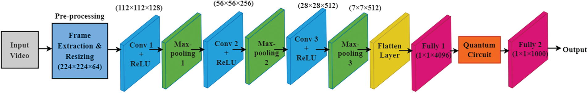
Figure 4: Architecture of the proposed QC-CNN model
• Convolutional layer
The most significant component of a CNN seems to be the convolution layer. This is the initial layer of a CNN that extracts features with a help of a convolution filter (also called the kernel) from the input (X × Y). From the input image, Kernels derive learnable parameters (such as weights) by employing forward propagation as well as backward propagation. To accomplish this task, a filter with size 3 × 3 has been dragged across the input matrix with stride 1. Element-wise matrix multiplication is performed and total the results at each step. A feature map is created as a result at the end.
The neuron value concerning position (x, y) in the jth feature map for layer i can be given as,
where t indexes the feature map in the (r − 1)th layer connected to the current (sth) feature map,
In the above equation, t denotes the feature map in the (r − 1)th layer linked to the present (sth) feature map,
• Activation function
Because most data in the actual world is nonlinear, activation functions are utilized to perform nonlinear data transformations. It ensures that the input space representation is mapped to a separate output space that meets the requirements. CNN uses a nonlinear activation function called the ReLU. This activation function’s result appears to be a continuous variable. When the input was negative, the output equals 0; else, the output is the same as the input. The ReLU function [30] is mathematically denoted as follows:
where x is the neuron’s input.
Another prominent consideration to utilize ReLU during the training of CNN is that it is much quicker than its competitors (sigmoid and tanh). All negative inputs are set to zero in ReLU, meaning that many nodes are ignored and will never be evaluated in future training.
• Pooling layer
A pooling layer is added between successive convolutional layers and is not trainable. The goal of introducing a pooling layer appears to be to lower the number of parameters and the network’s computing cost. This layer works independently on each input slice to resize it spatially. A filter with a size of 2 × 2 as well as a stride of 2 has been the most common sort of pooling layer. Every input depth slice, as well as the height and breadth, is down-sampled by two in each step. Pooling processes include max-pooling, average pooling, and min-pooling, among others. The CNN model employs the max-pooling, computed over every 2 × 2 tiny region in a depth slice.
To determine the output dimension of the max-pooling operation, the below mathematical expression can be utilized [31]:
where
• Fully connected layer and Quantum circuit
The suggested model includes two fully connected layers, one of which is put before the quantum layer and the other placed after it. These layers can be used to modify the quantum layer’s input and output sizes so that they correspond to the number of classes needed by the chosen dataset. To put it differently, the purpose of these two classical neural layers is to provide the coexistence of classical and quantum layers in the structure of the model. Also, it enables data embedding from the image space to the quantum capacity. In fully connected layers, all nodes of a layer engage and are linked to all other nodes of succeeding levels to make choices (classification, feature extraction). This help to determine the general connection of the characteristics. We add two fully linked non-linear layers to guarantee that these nodes communicate smoothly and account for all potential dependencies at the feature level.
In terms of the quantum component, the quantum layer (Quantum Circuit) seeks to profit from the qualities of probabilistic QC. This will detect and classify the anomaly types from the extracted feature vector. The classified anomaly types are Burglary, Fighting, Abuse, Robbery, Arson, Shooting, Assault, Shoplifting, Explosion, and Vandalism.
The performance standards as well as the empirical results of the proposed QC-CNN are discussed in this section. The proposed model’s effectiveness is quantitatively assessed via well-quality metrics such as the recall, confusion matrix, F1-score, precision, accuracy, ROC, and AUC.
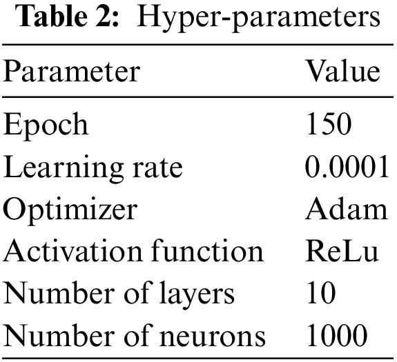
The models were trained on Google Colaboratory using Python’s sklearn package (version 1.0.2), and each user may expect: 1) a GPU Tesla 82 with 2498 CUDA cores, compute 3.7, 12-G GDDR5 VRAM; 2) a CPU single-core hyper threaded, i.e., (one core, two threads) Xeon Processors @2.20 GHz (No Turbo Boost); 3) 45-MB Cache; 4) 12.4 GB of accessible RAM; as well as 5) 320 GB of storage available. Every QCNN classifier, independent of the circuit used, was given training for 100 epochs with the Adam optimizer and a learning rate of 0.0001 using cross-entropy as the loss function. The CNNs were trained in the same manner, but it took 150 epochs for them to converge. The simulation parameters are provided in Table 2.
The confusion matrix has been regarded to be excellent, nevertheless, a straightforward objective metric that might be helpful when using any classification scheme. That measure provides a detailed understanding of how fine the classifier has been doing. And it is crucial to keep track of this while evaluating any classifier. As a result, this section gives an efficiency assessment of the proposed QC-CNN classifier using confusion matrix evaluation.
The confusion matrices derived from the dataset using the proposed technique are shown in Fig. 5. The suggested approach could only accurately identify every class, and also that anomalous classes are appropriately identified. For example, class vandalism is completely recognized, while class shoplifting is detected with 98% respectively. Unfortunately, the performance drops when the arson class is classified; nonetheless, considering that it achieves maximum accuracy with this dataset, the performance is appropriate.
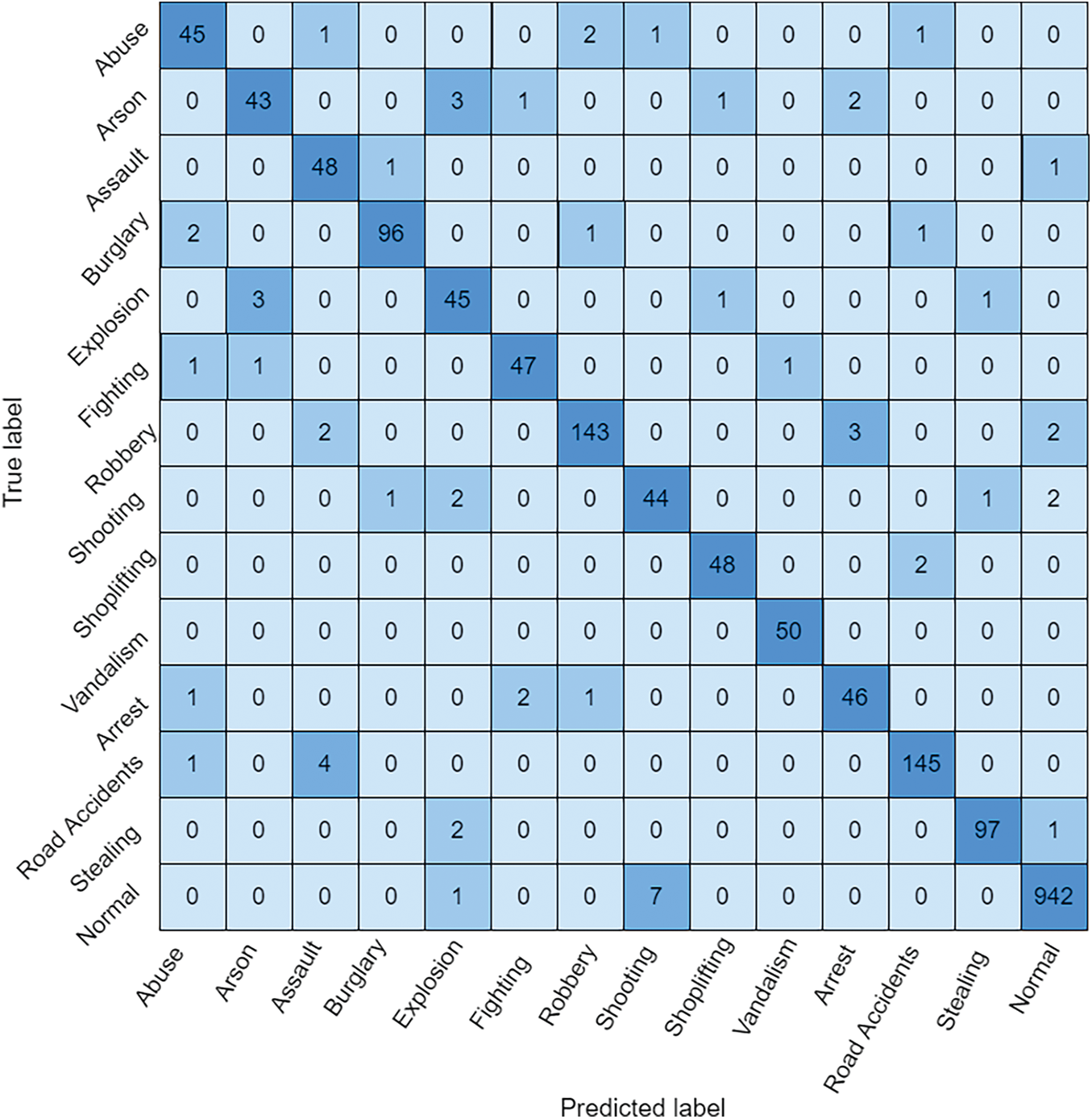
Figure 5: Confusion matrix for proposed QC-CNN
4.2 Accuracy Comparison of the Proposed Model with Classical Models
In classifying tasks accurately, the following factors are taken into account: true positives (TP), which are the correct inferences and actual results; false positives (FP), which are the correct inferences but are incorrect in reality; false negatives (FN) are incorrect inferred results, but the actual results are correct; and true negatives (TN), which are incorrect inferred and actual results.
Accuracy can be formulated as,
The proposed QC-CNN model is compared with classical models such as CNN [19], Autoencoder [19], GoogleNet with One-Class Support Vector Machines (OCSVM) [20], Histogram of Oriented Gradients (HOG) with One-Class Support Vector Machines (OCSVM) [20] and RGB and Flow two-stream networks [21]. When compared to these models in terms of accuracy, precision, recall, and F1 score, QC-CNN produces better results, which is shown in Table 3. All these models were evaluated on the UCF-crime dataset.
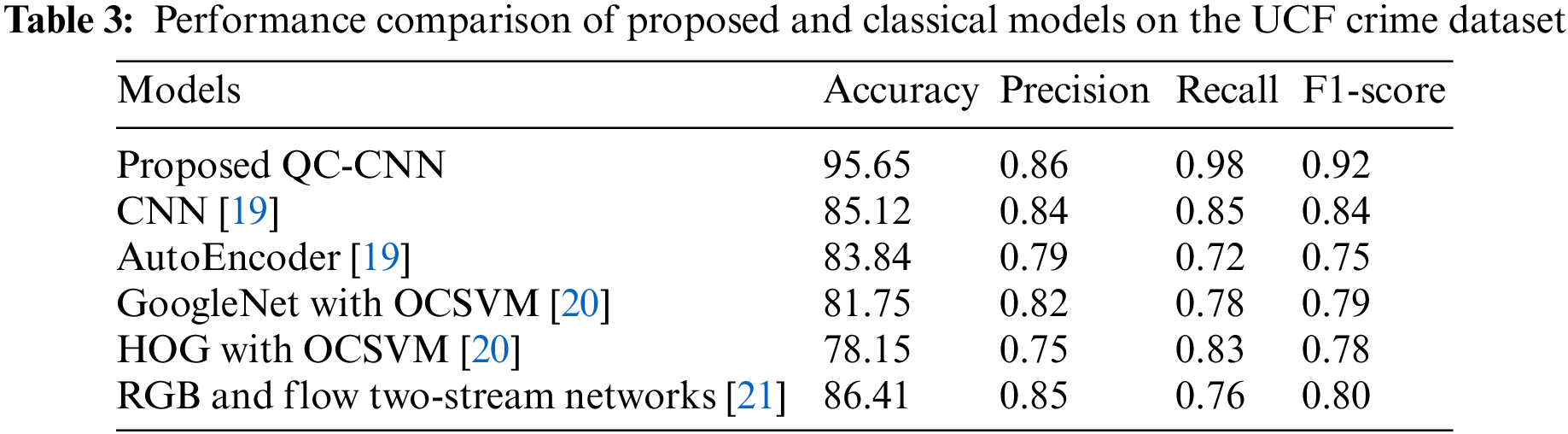
The hybrid QC-CNN has the ability to learn finer information to class images from the dataset with less complexity. The quantum gates can influence the final results and help speed up certain computational processes. The accuracy of QC-CNN is 10%, 11.81%, 13.9%, 17.5%, and 9.24% higher than CNN, autoencoder, GoogleNet with OCSVM, HOG with OCSVM and RGB, and Flow two-stream networks respectively. Also, the F1-score of the proposed QC-CNN is high which shows the efficiency of the model in classifying anomaly types from the surveillance video.
As the complexity of the problem grows, the speed requirements also increase in machine learning models. When compared to classical models, the proposed quantum machine learning models provide a more complex solution faster (huge volumes of data). This is because quantum superposition states allow for the manipulation of all possible combinations of a set of bits in a single operation, which speeds up the process of the models when compared to classical models. The proposed QC-CNN uses quantum properties of the quantum circuit to reduce model training time. Entanglement in quantum computing also aids in the automatic determination of hyperparameters. When compared to other models, quantum circuits perform faster and produce more accurate results. In a noisy environment, it also produces accurate results with a fixed memory dimension.
4.3 Accuracy Comparison of the Proposed Model with Quantum Models
In this work, the proposed QC-CNN and existing models such as Quantum Generative Adversarial Network (QGAN) [23], Hybrid classical-quantum Autoencoder (HAE) model [24], Quantum-assisted Neural Networks (QANN) [25], Quantum orthogonal neural network (QONN) [25] are compared. The dataset and application used in these existing models are different from the proposed work.
The authors of [23] proposed a QGAN model for a human-centered paradigm that is implemented in the cloud for the synthetic dataset. The authors of [24] suggested an HAE approach as well as four datasets to monitor gas power stations. For medical image classification, two models, QONN and QANN, were proposed in [25]. All of the existing methods are based on quantum machine learning and serve different purposes. There are no existing quantum machine learning models in video surveillance applications, as far as we know. So, using the UCF-crime dataset, this work evaluated and compared the proposed work with these existing methods. As a result, the comparison is provided in Tables 3–9, as well as Figs. 6–9.

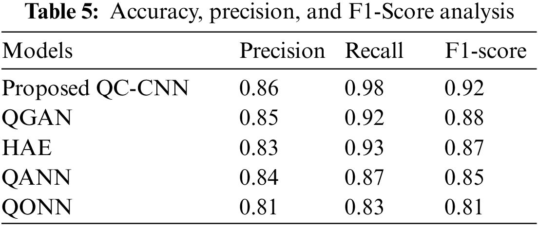
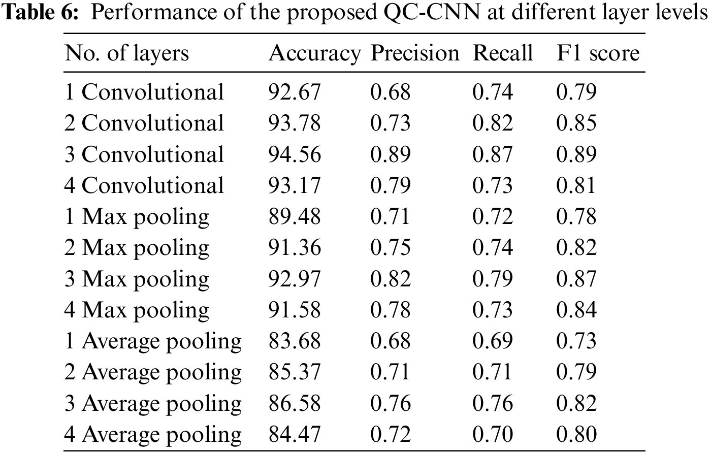
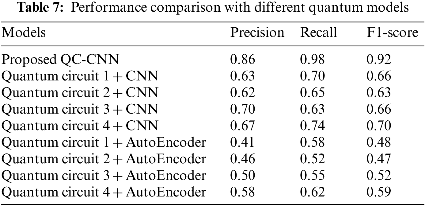
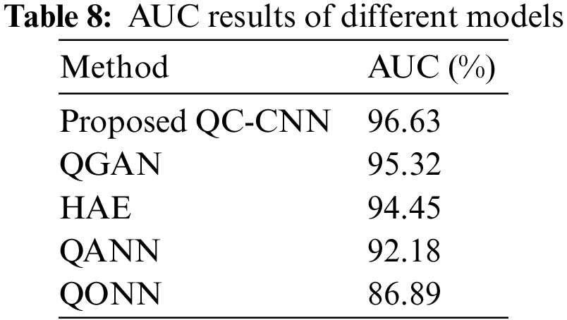
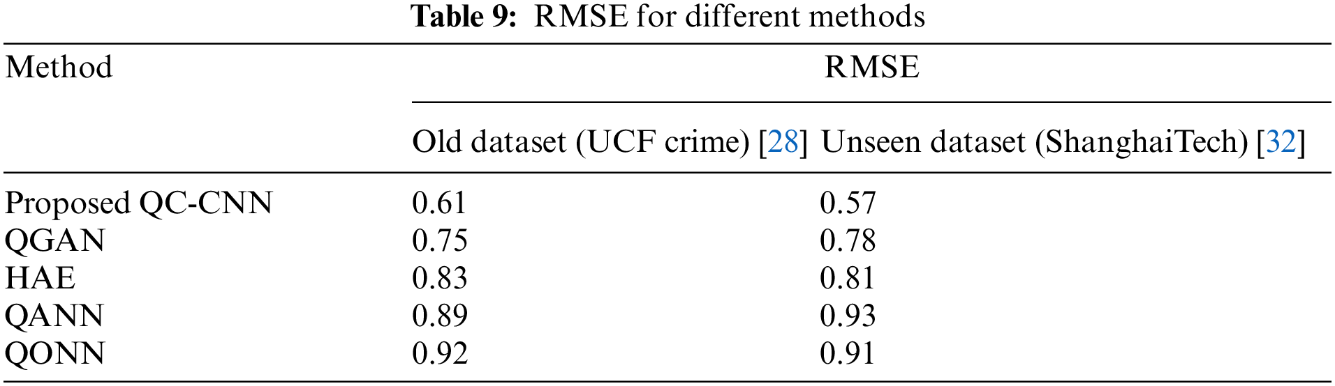
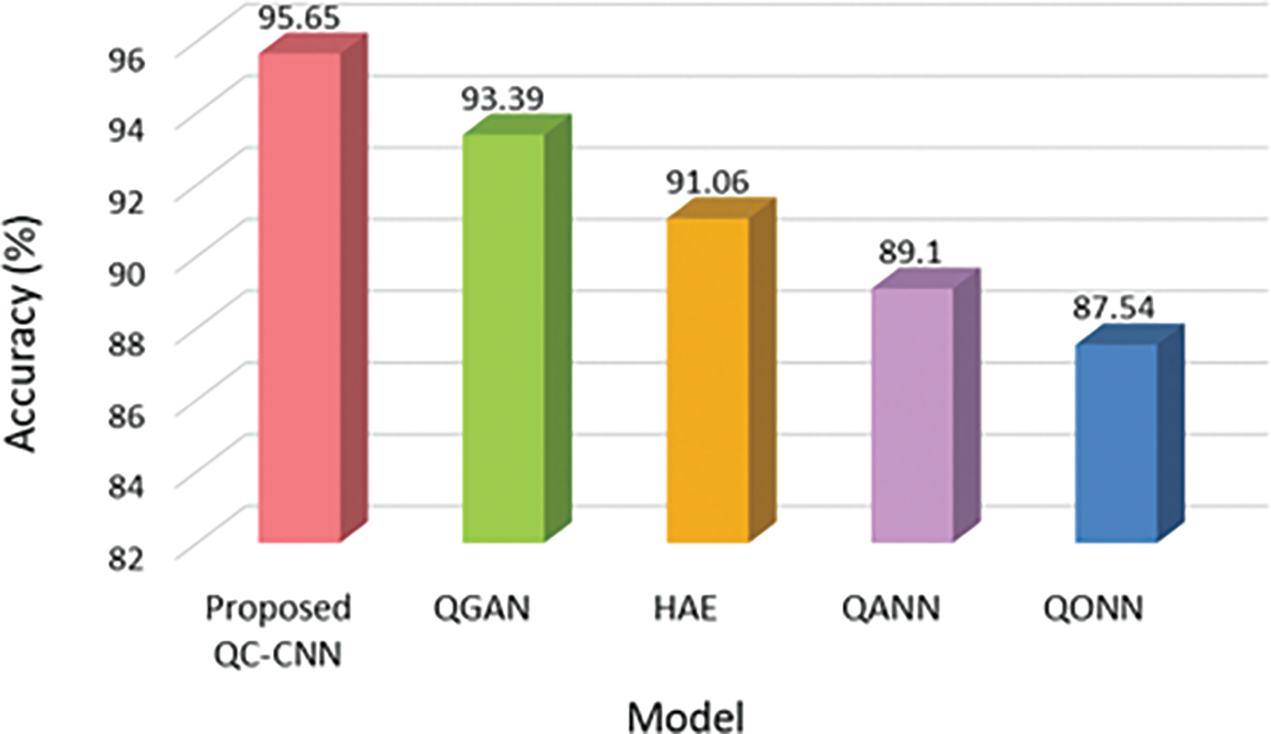
Figure 6: Comparison of accuracy with other models
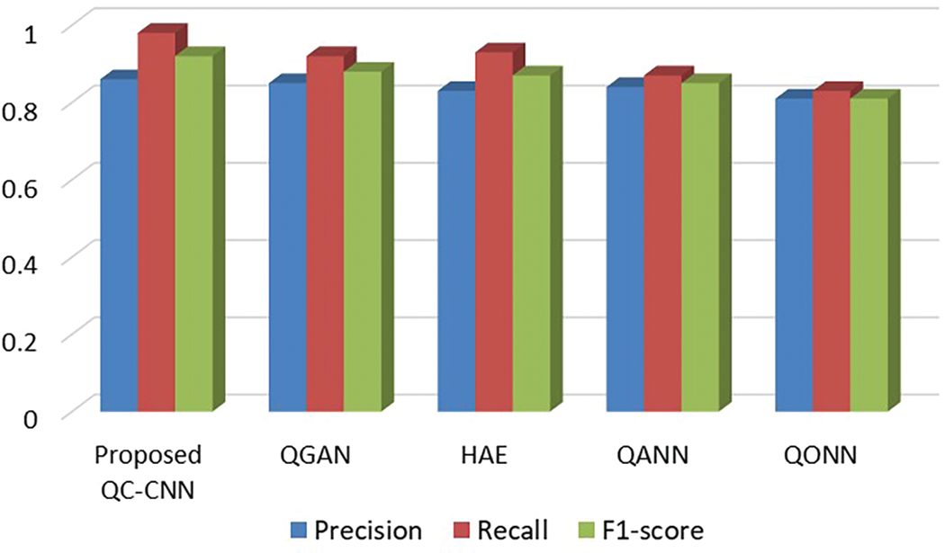
Figure 7: Results obtained for the precision, recall, and F1-score for various methods
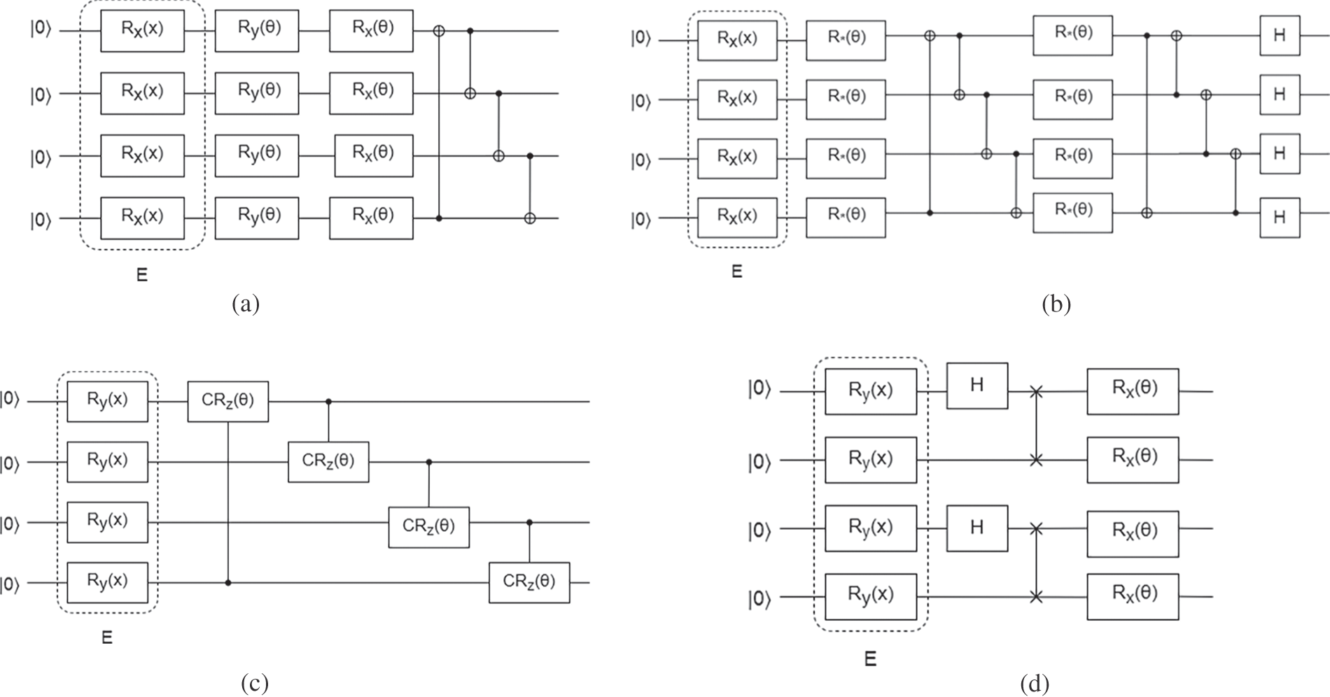
Figure 8: Quantum circuits (a) Quantum circuit 1 (b) Quantum circuit 2 (c) Quantum circuit 3 (d) Quantum circuit 4
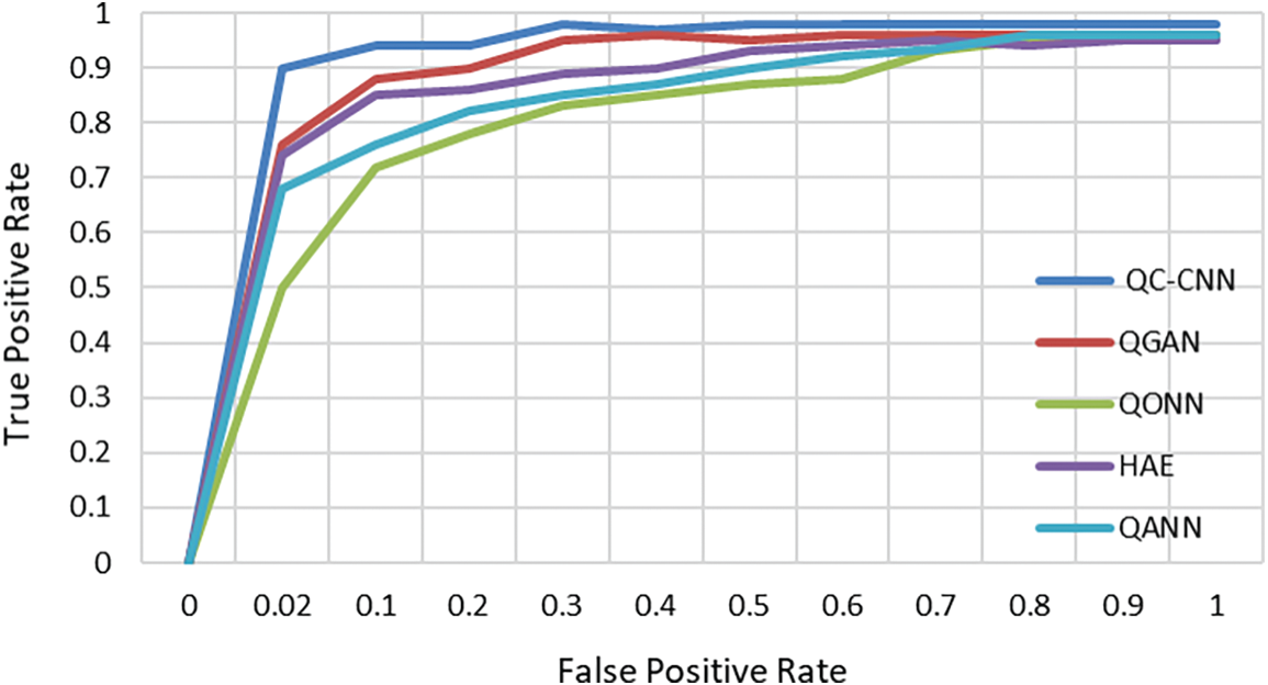
Figure 9: ROC curves of different models
From Fig. 6, it is clear that QC-CNN achieved the highest accuracy of 95.65%, which is 2.26%, 4.59%, 6.55%, and 8.11% higher than QGAN, HAE, QANN, and QONN, respectively. This is because the data is first pre-processed, then deep spatio-temporal features are extracted during training. Also, the proposed method eliminates the overfitting problem, which further increases the model’s accuracy. It is important to note that the architecture described in this research is far less complicated than other approaches.
4.4 Precision, Recall, and F1-Score
The recall can be defined as the proportion of entire outcomes categorized properly with the help of a model. But, precision addresses the issue of how frequently a model is true if it forecasts yes. To completely evaluate the model’s performance, it is necessary to examine the accuracy as well as recall. In this instance, the F1-score, which seems to be the harmonic mean of recall as well as precision, might be employed. The greater the score, the better the model. The percentage of correct predictions generated by the model is denoted as accuracy.
Recall, precision, and F1-can be formulated in Eqs. (11)–(13) as,
Table 5 depicts the performance of proposed and existing models in terms of precision, recall, and F1 score.
Fig. 7 illustrated the results obtained for proposed and existing methods with respect to precision, recall, and F1-score. The proposed model reached precision, recall, and F-score of 81%, 83%, and 81% respectively. It achieves continuously better results when compared to other techniques like QGAN, HAE, QANN, and QONN, indicating that the proposed QC-CNN can acquire finer features to identify comparable images with constant complexity on a real-world dataset. Also, the proposed QC-CNN is less complex and has few parameters.
4.5 Performance Comparison with Different Numbers of Layers
The following are the experiments made for the proposed QC-CNN with a different number of convolutional and pooling layers which is shown in Table 6.
Adding more layers will aid in the extraction of deeper features. However, it is possible to do so to a certain extent. There is a limit. Instead of extracting features, it then tends to ‘overfit’ the data. Overfitting can result in errors of various types, such as false positives. We tested the proposed system’s performance by increasing the number of layers from one to four. While adding layers, the performance gradually improves. When three layers are used, the proposed QC-CNN produces the best results. Following that, adding layers reduces performance due to the overfitting issue. As a result, the model is fitted to three layers. Since the average pooling approach smoothes down the image, the sharp features may be lost. Max pooling chooses the brightest pixels in the image. It is helpful when the backdrop of the image is dark and we are only interested in the image’s lighter pixels. Average pooling cannot always extract the important features because it considers everything and returns an average value that may or may not be significant. Max pooling concentrates on the most important features. Even though max-pooling is a non-linear operation, it is primarily used to decrease the dimensionality of the input, thereby reducing overfitting and computation. As a result, in our proposed algorithm, max pooling outperforms average pooling.
4.6 Performance Comparison with Different Quantum Models
Table 7 shows the comparison of different quantum circuit models with classical network structures. The performance of four quantum circuits such as quantum circuits 1, 2, 3, and 4 with CNN and autoencoder are compared and evaluated in terms of precision, recall and F1-score. Table 7 demonstrates that the proposed QC-CNN using a real amplitude circuit had the maximum recall and precision of the circuits evaluated. The suggested QC-CNN showed high performance on the evaluated dataset. This shows that the proposed QC-CNN with a real amplitude circuit outperforms the other existing model. Fig. 8 shows the different quantum circuits used for comparison.
4.7 Receiver Operating Characteristic (ROC) and Area Under Curve (AUC)
The ROC curve seems to be a probability graph that represents a classification model’s accuracy across all classification criteria. This graph compares the true positive rate with the false positive rate. The higher the true positive rate, the better the detection efficiency. The lower the false positive rate, the steeper the ROC curve.
The AUC is a classification strategy measure. After accuracy, it is the second most common statistic. Fig. 9 illustrates the ROC curve for various models. QC-CNN outperforms better when compared to other models such as QANN, HAE, QONN, and QGAN. The actual positive and false positive rates were computed to evaluate the model’s performance. The proposed method, as shown in Fig. 9, achieves a good balance between the actual positive rate and false positive rate, making it more suitable for anomaly detection surveillance systems.
Table 8 shows AUC’s performance results, in which the proposed QC-CNN achieves the highest value of 96.63% compared to other models. This additionally gives a quantitative performance analysis of the proposed model.
A trustworthy analysis should provide an appropriate prediction (prediction with the least amount of error) for any type of test input. To validate the suggested model’s reliability, one of the reliable metrics Root Mean Square Error (RMSE) is used to measure the success of predictive models. The RMSE is a common approach for assessing a model’s error in forecasting quantitative data. The formal definition is as follows:
where n stands for the total number of samples,
According to Table 9, the suggested approach has a low RMSE error rate when compared to other methods. The suggested model performs well on both known and unknown or new datasets. This is because the suggested model performs accurate prediction by adjusting hyper-parameters and hidden layer adjustments repeatedly until optimal results are obtained, as shown in Table 9. The suggested model is highly reliable to use for classification based on its RMSE value.
The Population Stability Index (PSI) is used to determine the stability of the proposed model by assessing how the population or features have changed within the framework of the model. It is a term for determining how much a variable’s distribution has moved between two samples over time. It is extensively used for monitoring changes in population features and detecting potential problems with model performance. It is often a useful indicator of whether the model has stopped forecasting effectively owing to large changes in population distribution.
Using the following equation, calculate the PSI for each kind of anomaly:
where
Various actions and measures may be taken depending on the outcome. If the outcome is satisfactory, there is no need for more action. If the result is not satisfactory, additional detailed analysis will be required, based on whether a score or individual score component was evaluated for PSI. The PSI for the QC-CNN model was estimated in Table 10.
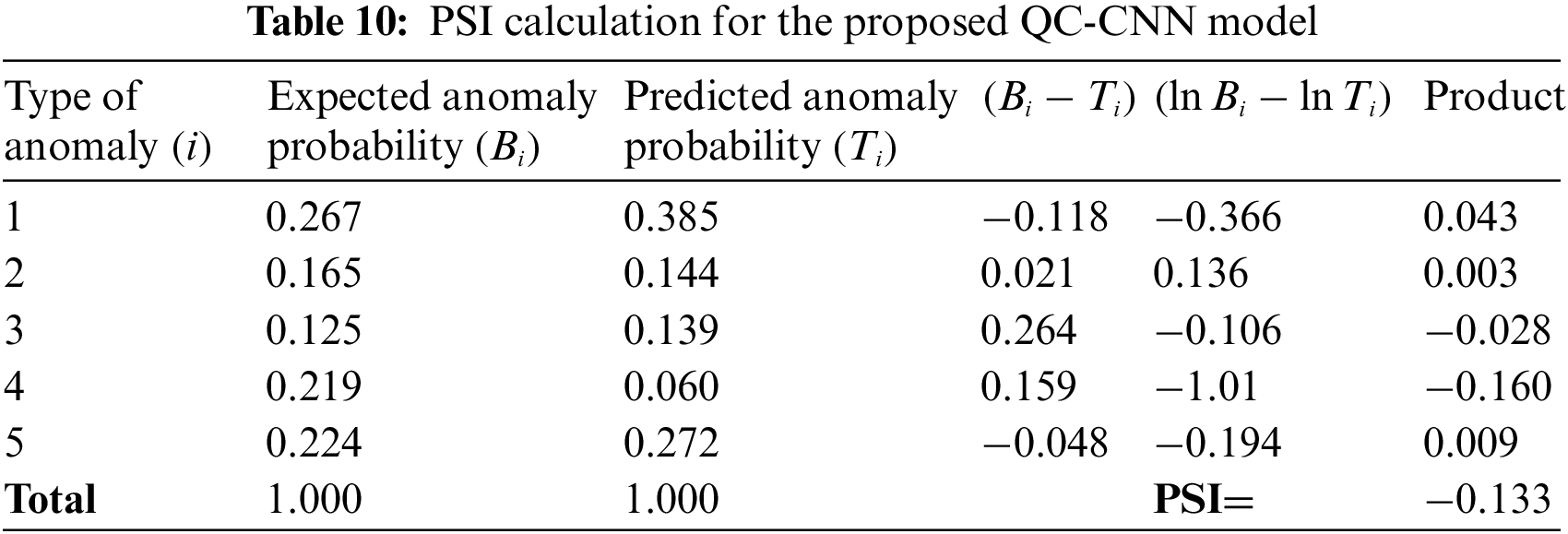
Table 10, 1, 2, 3, 4, and 5 represent five types of anomalies namely Shoplifting, Assault, Vandalism, Fighting, and Burglary respectively. The PSI value is estimated with the help of expected and predicted anomaly probability values. Here the PSI value is −0.133 which is less than 1. It satisfied the above condition PSI < 0.1 which indicates the model is stable and the population hasn’t changed, so keep the model as it is. This indicates the effectiveness of the model in terms of stability.
This work investigates the hybrid quantum computing-based deep learning model for anomaly classification in surveillance videos. Unlike traditional CNN, this work uses a quantum circuit as one of the quantum layers in CNN for multi-class types. This increases overall accuracy and reduces the computational efficiency of the proposed QC-CNN model. Furthermore, experimental findings reveal that the QC-CNN outperforms the UCF-Crime dataset in the confusion matrix, accuracy, precision, recall, F1-score, ROC, and AUC. The accuracy of the QC-CNN is 95.65%, which is 2.26%, 4.59%, 6.55%, and 8.11% greater than the QGAN, HAE, QANN, and QONN, accordingly. As a result, the proposed QC-CNN outperforms other current models in overall classification accuracy of about 5.37%. In addition, the suggested method’s effectiveness is tested by altering the number of layers in CNN and comparing it to quantum and classical models. Future studies will seek to increase the quantum processing component’s contribution to the hybrid approach. Furthermore, more sophisticated quantum circuits are expected to improve the model’s learning capabilities.
Acknowledgement: The authors wish to express their thanks to one and all who supported them during this work.
Funding Statement: The authors received no specific funding for this study.
Conflicts of Interest: The authors declare that they have no conflicts of interest to report regarding the present study.
References
1. T. Ganokratanaa, S. Aramvith and N. Sebe, “Unsupervised anomaly detection and localization based on deep spatiotemporal translation network,” IEEE Access, vol. 8, pp. 50312–50329, 2020. [Google Scholar]
2. W. Ullah, A. Ullah, I. U. Haq, K. Muhammad, M. Sajjad et al., “CNN features with Bi-directional LSTM for real-time anomaly detection in surveillance networks,” Multimedia Tools and Applications, vol. 80, no. 11, pp. 16979–16995, 2020. [Google Scholar]
3. R. Maqsood, U. I. Bajwa, G. Saleem, R. H. Raza and M. W. Anwar, “Anomaly recognition from surveillance videos using 3D convolution neural network,” Multimedia Tools and Applications, vol. 80, no. 12, pp. 18693–18716, 2021. [Google Scholar]
4. N. Nasaruddin, K. Muchtar, A. Afdhal and P. Dwiyantoro, “Deep anomaly detection through visual attention in surveillance videos,” Journal of Big Data, vol. 7, no. 1, pp. 1–17, 2020. [Google Scholar]
5. C. Wu, S. Shao, C. Tunc, P. Satam and S. Hariri, “An explainable and efficient deep learning framework for video anomaly detection,” Cluster Computing, vol. 25, pp. 2715–2737, 2022. [Google Scholar]
6. K. Deepak, G. Srivathsan, S. Roshan and S. Chandrakala, “Deep multi-view representation learning for video anomaly detection using spatiotemporal autoencoders,” Circuits, Systems, and Signal Processing, vol. 40, no. 3, pp. 1333–1349, 2020. [Google Scholar]
7. A. Ravi and F. Karray, “Exploring convolutional recurrent architectures for anomaly detection in videos: A comparative study,” Discover Artificial Intelligence, vol. 1, no. 1, 2021. [Google Scholar]
8. A. Ramchandran and A. K. Sangaiah, “Unsupervised deep learning system for local anomaly event detection in crowded scenes,” Multimedia Tools and Applications, vol. 79, no. 47–48, pp. 35275–35295, 2019. [Google Scholar]
9. M. Asad, H. Jiang, J. Yang, E. Tu and A. A. Malik, “Multi-stream 3D latent feature clustering for abnormality detection in videos,” Applied Intelligence, vol. 52, no. 1, pp. 1126–1143, 2021. [Google Scholar]
10. F. Rezaei and M. Yazdi, “Real-time crowd behavior recognition in surveillance videos based on deep learning methods,” Journal of Real-Time Image Processing, vol. 18, no. 5, pp. 1669–1679, 2021. [Google Scholar]
11. F. R. Bento, R. F. Vassallo and J. L. Samatelo, “Anomaly detection on public streets using spatial features and a bidirectional sequential classifier,” Journal of Control, Automation and Electrical Systems, vol. 33, no. 1, pp. 156–166, 2021. [Google Scholar]
12. Z. Qin, H. Liu, B. Song, M. Alazab and P. M. Kumar, “Detecting and preventing criminal activities in shopping malls using massive video surveillance based on deep learning models,” Annals of Operations Research, 2021. [Google Scholar]
13. IBM. What is quantum computing? Accessed: Jun. 20, 2021. [Online]. Available: https://www.ibm.com/quantum-computing/what-is-quantumcomputing/. [Google Scholar]
14. R. Parthasarathy and R. T. Bhowmik, “Quantum optical convolutional neural network: A novel image recognition framework for quantum computing,” IEEE Access, vol. 9, pp. 103337–103346, 2021. [Google Scholar]
15. H. Chen, L. Wossnig, S. Severini, H. Neven and M. Mohseni, “Universal discriminative quantum neural networks,” Quantum Machine Intelligence, vol. 3, no. 1, pp. 1–11, 2020. [Google Scholar]
16. J. Amin, M. Sharif, N. Gul, S. Kadry and C. Chakraborty, “Quantum machine learning architecture for COVID-19 classification based on synthetic data generation using conditional adversarial neural network,” Cognitive Computation, vol. 14, no. 5, pp. 1677–1688, 2021. [Google Scholar]
17. A. Chalumuri, R. Kune, S. Kannan and B. S. Manoj, “Quantum-enhanced deep neural network architecture for image scene classification,” Quantum Information Processing, vol. 20, no. 11, 2021. [Google Scholar]
18. Y. Wang, X. Liang, X. Hei, W. Ji and L. Zhu, “Deep learning data privacy protection based on homomorphic encryption in AIoT,” Mobile Information Systems, vol. 2021, pp. 1–11, 2021. [Google Scholar]
19. J. Jeong, S. Kwon, M. Hong, J. Kwak and T. Shon, “Adversarial attack-based security vulnerability verification using deep learning library for multimedia video surveillance,” Multimedia Tools and Applications, vol. 79, no. 23–24, pp. 16077–16091, 2019. [Google Scholar]
20. A. Chriki, H. Touati, H. Snoussi and F. Kamoun, “Deep learning and handcrafted features for one-class anomaly detection in UAV video,” Multimedia Tools and Applications, vol. 80, no. 2, pp. 2599–2620, 2020. [Google Scholar]
21. W. Hao, R. Zhang, S. Li, J. Li, F. Li et al., “Anomaly event detection in security surveillance using two-stream based model,” Security and Communication Networks, vol. 2020, pp. 1–15, 2020. [Google Scholar]
22. S. Vosta and K. Yow, “A CNN-RNN combined structure for real-world violence detection in surveillance cameras,” Applied Sciences, vol. 12, no. 3, pp. 1021, 2022. [Google Scholar]
23. W. Liu, Y. Zhang, Z. Deng, J. Zhao and L. Tong, “A hybrid quantum-classical conditional generative adversarial network algorithm for human-centered paradigm in cloud,” EURASIP Journal on Wireless Communications and Networking, vol. 1, pp. 1–17, 2021. [Google Scholar]
24. A. Sakhnenko, C. O’Meara, K. J. B. Ghosh, C. B. Mendl, G. Cortiana et al., “Hybrid classical-quantum autoencoder for anomaly detection,” arXiv[Quantum Physics], 2021. [Google Scholar]
25. N. Mathur, J. Landman, Y. Y. Li, M. Strahm, S. Kazdaghli et al., “Medical image classification via quantum neural networks,” arXiv [Quantum Physics], 2021. [Google Scholar]
26. S. Y. C. Chen, C. H. H. Yang, J. Qi, P. Y. Chen, X. Ma et al., “Variational quantum circuits for deep reinforcement learning,” IEEE Access, vol. 8, pp. 141007–141024, 2020, https://doi.org/10.1109/ACCESS.2020.3010470. [Google Scholar]
27. H. Yano, Y. Suzuki, K. M. Itoh, R. Raymond and N. Yamamoto, “Efficient discrete feature encoding for variational quantum classifier,” IEEE Transactions on Quantum Engineering, vol. 2, pp. 1–14, 2021, Art no. 3103214, https://doi.org/10.1109/TQE.2021.3103050. [Google Scholar]
28. M. U. Meraj, Anomaly-detection-dataset-UCF. Kaggle: Your Machine Learning and Data Science Community, 2022. [Online]. Available: https://www.kaggle.com/datasets/minhajuddinmeraj/anomalydetectiondatasetucf. [Google Scholar]
29. A. Sebastianelli, D. A. Zaidenberg, D. Spiller, B. Le Saux and S. Ullo, “On circuit-based hybrid quantum neural networks for remote sensing imagery classification,” IEEE Journal of Selected Topics in Applied Earth Observations and Remote Sensing, vol. 15, pp. 565–580, 2022. [Google Scholar]
30. D. R. Sarvamangala and R. V. Kulkarni, “Convolutional neural networks in medical image understanding: A survey,” Evolutionary Intelligence, vol. 15, no. 1, pp. 1–22, 2021. [Google Scholar]
31. M. M. Rahman, M. S. Islam, R. Sassi and M. Aktaruzzaman, “Convolutional neural networks performance comparison for handwritten bengali numerals recognition,” SN Applied Sciences, vol. 1, no. 12, 2019. [Google Scholar]
32. W. Luo, W. Liu and S. Gao, “A revisit of sparse coding-based anomaly detection in stacked RNN framework,” in Proc. of the Int. Conf. on Computer Vision, Venice, Italy, October 2017. [Google Scholar]
Cite This Article
 Copyright © 2023 The Author(s). Published by Tech Science Press.
This work is licensed under a Creative Commons Attribution 4.0 International License , which permits unrestricted use, distribution, and reproduction in any medium, provided the original work is properly cited.
 Downloads
 Citation Tools