Automatic Sentimental Analysis by Firefly with Levy and Multilayer Perceptron

1  Introduction

There has been an increase in the availability of data sources with strong opinions, including personal blogs, online review sites, and microblogging platforms due to the rise of social networking sites. A broad set of concerns are addressed, opinions are conveyed, complaints were made, and recommendation and feedbacks are supplied for products and policies that everyone uses or that worry them on a daily basis. The common attitude towards a certain issue is ascertained using data from unstructured social media. Sentiment analysis (SA) [1] is an intelligence mining approach that is used, for instance, to record and ascertain users’ opinions and sentiments regarding a particular subject or incident. Regular and irregular language patterns and in-depth knowledge of syntax, semantics, implicit and explicit grammatical norms, are necessary for social media sentiment mining, which is labor-intensive. Gathering information on opinions of people, choosing features, categorising those feelings, and figuring out how polarised those feelings are all processes in the SA process. Features selection is important in SA since opinionated articles generally have high dimension. The effectiveness of SA classifiers is harmed by this. The implementation of a successful feature selection technique as a result results in a shorter training time for the classifier. This text classification difficulty grows as a result of social media material being unstructured and high-dimensional, prompting the quest for better and more efficient feature selection algorithms [2]. Traditional techniques like chi-square and mutual information [3] might be useful if you want to diminish the corpora size without compromising the performance. Selecting feature subsets for non-polynomial-hard (NP) problems results in inadequate feature subsets. Evolutionary algorithm has been successful in assessing how well the solutions to difficult issues are [4]. Genetic algorithms [5,6], simulated annealing, and nature-inspired algorithms [7] have all been thoroughly investigated to enhance categorisation. In a distributed system known as swarm intelligence, anonymous social agent interact locally and sense the environment to create self-coordinating global behaviour [8].

The Firefly algorithm (FA) was created on the basis of flashing patterns of the fireflies. This ecologically inspired algorithm. Swarm intelligence algorithms typically outperform one another; however, the FF algorithm is a relatively new one. It uses a firefly pattern to symbolise potential solutions in the search space as a population-based metaheuristic method [9]. In this article, Firefly with Levy and Multilayer Perceptron algorithms were used to automate SA through feature their neighbors and their surroundings to prod-cooperating global behavior [8] ect relevant TCs and concentrate them on the relevant experiments. For the purpose of automating SA, Section 2 of this article describes feature extraction from related work and a classification model based on selection. In Section 3, it is detailed how to extract features, choose features based on FF criteria, and categorise data using MLP. The proposed FF-MLP model for SA calculation and how it is organised to remove irrelevant information are also covered. The SA calculation method's Performance Validation of the FF-MLP model is described in Section 4 of the document. Sensitivity, accuracy, specificity, and F1 Score are all improved by the Firefly with Levy and Multilayer Perceptron methodology that is being presented. Division 5 has demonstrated the conclusion.

2  Literature Review

Most user-generated data is now accessible due to social media’s quick surge in popularity. It will take a lot of work for sorting the data and ascertain the feeling over it. “Text” is the popular online data format for conveying people’ ideas and opinions in a clear manner [10]. This work focuses on a thorough analysis of machine learning-based SA algorithms and approaches [11]. The algorithm becomes more flexible as the inputs vary. Various techniques use different data labelling and processing methods, including n-grams, bigrams, and unigrams. The majority of the time, positive and negative opinions are classified and forecast using machine learning (ML) algorithms. ML algorithms can be further categorised, according to [12].

Based on the training dataset, the input dataset was labelled with the output class or results that contains pre-labeled classes [13]. The proposed technique uses a training classifier to categorise the incoming dataset. The input item and the anticipated output results are both included in the training data set [14]. The training dataset can be analyzed by means of supervised learning techniques to produce a conditional function which can then be exploited for mapping new dataset, generally called as test dataset. The Supervised approach is frequently employed in ML approaches. Regression and classification are two techniques for categorising data. Techniques for supervised ML include support vector machines, random forests, and linear regression. These ML algorithms use unlabelled dataset to find patterns and structures that are otherwise hidden. This approach trains the classifier using unlabelled data as opposed to supervised learning. Two of the most popular unsupervised ML algorithms, which are further divided into clustering and association, are K-Means and the Apriori Algorithm [15].

Algorithms that are semi-supervised work with both labelled and unlabelled sources of data. Various lexicon-based tools were used to examine the features and accuracy [16]. This study investigates and analyses several ML methodologies and algorithms to take things a step further. A thorough comparison of different techniques and accuracy levels is also done. The technique of classifying unstructured data and language as good, negative, or neutral is known as opinion mining. Much of this work has previously been completed using SA and ML methods [17]. Due to the countless chances for unrestricted expression of ideas and beliefs that social networking platforms like Facebook and Twitter offer, people from throughout the world have flocked to them in recent years. According to [18,19] most emotions are categorised as either good or negative.

Maximizing Entropy (MaxEnt) is a feature enabled sentiment classification approach that does not need independent assumption, according to [20–22]. Method of ML Even if the classifier’s loss function is non-differentiable, Stochastic Gradient Descent (SGD) can force it to learn [23]. Classification tree can be enriched and stored using Random Forest, which was first proposed in [24]. Reference [25] mentions SailAil Sentiment Analyser as another ML-based sentimental classification system (SASA). An effective and non-linear neural network model based on ML is the MLP algorithm. A well-known ML algorithm called Naive Bayes was first proposed by Thomas Bayes [26]. One of the most often used supervised ML methods is the support vector machine (SVM). The use of different algorithms or tools in ML-based SA has been the subject of many researches. Contrarily, SVM fared better than the others in terms of accuracy and effectiveness, according to [27].

In recent years, researchers and industry professionals have given SA a lot of consideration. The ABC approach for feature selection enhanced classification performance and minimised computational cost by determining the ideal feature set via optimal set of features [28]. A powerful optimizer methods like ABC are frequently applied to NP-hard issues. To optimise the benefits of opinion mining, the ABC approach is utilised to categorise movie reviews. This strategy improved classification accuracy by 1.63–3.81 percent. In order to compute sentiment weight, the ABC technique was investigated in this study [29]. The ABC approach was applied to boost the classifier performance, and the best classification result was optimised using BOW and BON characteristics. According to the experiments, accuracy rose from 55% to 70%. Aspect-based SA characteristics were chosen using particle swarm optimization [30]. This method can enhance sentiment categorization since it chooses the most important elements for SA automatically. A feature set with fewer dimensions increases system accuracy, according to experiments. Reference [31] uses a distance-based discrete FA to choose the mutual information criterion to determine the optimum features for text categorization [32,33].

In [34] proposed a Multi Feature Supervised Learning technique for resolving the targeted vehicles in a huge image gallery based on the appearance. Intelligent transportation has been improved with the use of fine-grained vehicle type categorization utilizing a CNN with feature optimization and joint learning approach [35]. A unique community information-based link prediction approach [36] uses the community information of every neighboring node to forecast the connection between the node pair. It has been suggested to use a variational autoencoder (VAE) enabled adversarial multimodal domain transfer (VAE-AMDT) to acquire more discriminating multimodal representation that also can enhance performance of the system, and it has been jointly trained with a multiattention mechanism to decrease the distance difference amongst the unimodal representation [37]. The sentiment feature set was employed to train and predict sentiment classification labels in a convolution neural network (CNN) and a bidirectional long short-term memory (BiLSTM) network [38].

3  The Proposed Firefly-Multilayer Perceptron Model

The FF-MLP technique for SA that is provided includes the pre-processing of online product reviews to weed out extraneous material, feature extraction, feature selection based on FF, and classification based on MLP. All extraneous information had to be removed before features could be extracted, including stop words, URLs, plenty of spaces, and hashtags. To remove the URL linkages, regular expression matching will be performed. The hashtag (#) and the majority of punctuation are eliminated in favour of blank space. The product review terms are then lowercased. Fig. 1 depicts the model diagram for the firefly-multilayer perceptron.

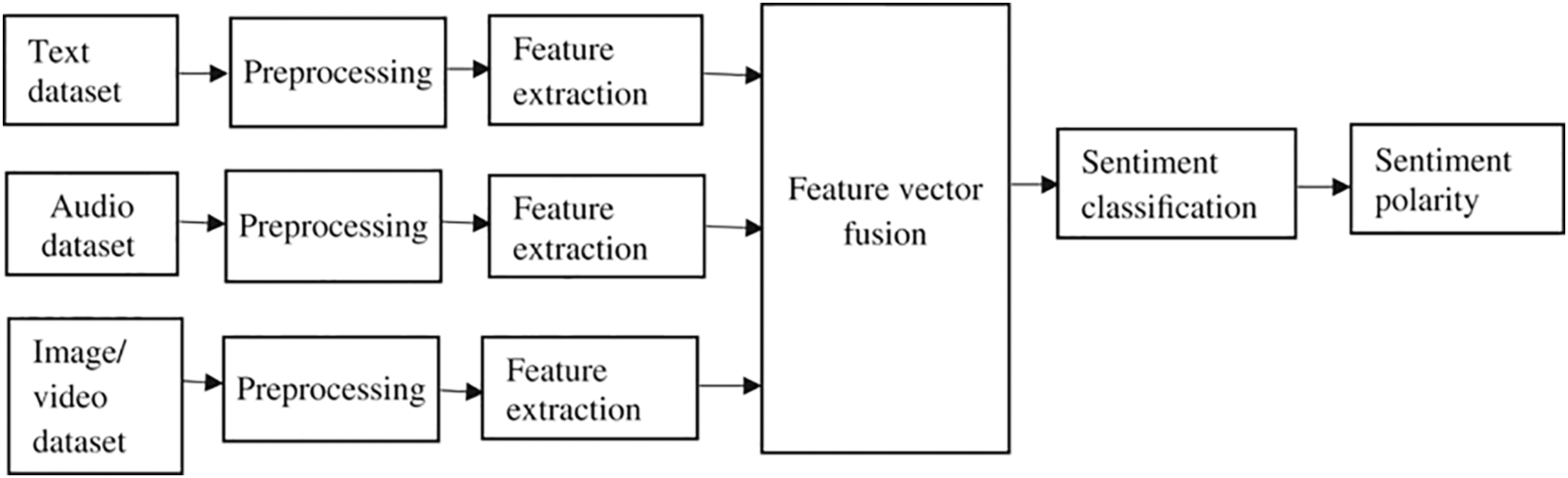
Figure 1: Model diagram for firefly-multilayer perceptron

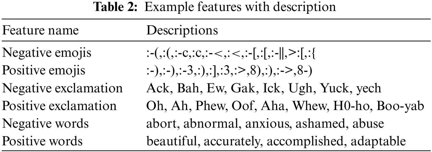
Additionally, terms like “is,” “a,” “the,” and so on that don’t start with an alphabetic letter should be eradicated. The dictionaries of stop word and acronyms are used to increase accuracy of the dataset. The pre-processed internet product reviews are utilised to create feature vectors from the dataset’s 10 computed features. Below is a list of the filtered feature datasets, including exclamation points, emojis, words, and character counts. FF is used to choose the features. Among the high-dimension feature subset, the best features can be selected for SA using the FF approach. The primary concept of the FF algorithm is to evaluate each sFF individually by using the illumination information of surrounding FFs. Any FF is pulled to its brighter neighbours depending on the distance threshold. In the conventional FF model, arbitrariness and absorption are used as control variables. Two important factors in confirming the FS issue are the time it takes to reach optimality and the optimality itself.

3.1 Artificial Firefly Algorithm

The real fireflies’ flashing lights served as the inspiration for the FA, a metaheuristic technique based on firefly behaviour. The two fireflies attract one other because of their illumination, which influences how well the algorithm performs. When designing an algorithm based on the behaviour of fireflies, we need to take into account three conditions that describe how fireflies behave in the real world. As for the guidelines:

•   A genderless insect, the firefly. Consequently, all fireflies will be drawn to one another, regardless of their gender.

•   Illumination is the antithesis of beauty, in this context. In any flash illumination, this makes the less dazzling firefly leave in favour of the more brilliant one. The attraction of a pair of fireflies grows as the distance amongst them widens. The fireflies will float about aimlessly if there isn’t a standout.

The illumination of firefly output is influenced or controlled by the fitness function’s terrain. It’s possible that the illumination in the maximisation problem is only inversely proportional to the fitness function value. Important elements of the FA include the light’s illumination and the firefly’s attraction. With respect to the firefly’s illumination, the light’s intensity varies from each source. Using a variation of the fitness function, it is expressed and computed. Light intensity, which controls illumination, governs attraction. Each firefly’s attraction is determined by using Eq. (1).

β=βoe−γd2(1)

The value 0 represents the β0 attractiveness (r) at a zero distance. There are some mathematical calculations that employ the number 1. The indicator shows how much light has been absorbed. I and j, two fireflies in distinct locations, are separated by r.

3.2 Firefly Levy-Flight Algorithm

The movement of fireflies from one place to another occurs constantly. Two fireflies are attracted to one another based on distance. It is possible to determine the separation between any two fireflies, I and j, using the Euclidean distance law [33], as demonstrated in Eq. (2):

duv=||pu−pv||=∑k=1r(pu,k−pv,k)2(2)

where pu,k signifies the kth components of the firefly u’s position and d indicates the problem’s dimension. They draw to one another because of their varying illumination levels when one of them is moved near the other. Eq. (3) [33] governs this movement, which is represented by the following:

pu=pu+βe−γuvd2(pu−pv)+αsign[rand−12]⊕Levy(3)

In Eq. (3), rand is a randomly generated number with a [0,1] range and coefficient is an arbitrary value that determines the random walking size. To reach the higher one, the lower illumination firefly must wait three terms [33]. The existing location of the low-light firefly will be discussed first. The attraction coefficient dictates the firefly’s preference towards brighter lights. A random generator multiplied by generates a random walking in the last term, which is the result of the process.

3.3 Firefly Levy Based Feature Selection Process

A discrete FA can be used to solve the FS problem. In this instance, the correctness of the response u in terms of its fitness is evaluated using the fitness function f. The FF parameters population (N), tmax—maximal amount of generations, γ—absorption coefficient, and α—arbitrariness necessary for halting criterion—are all initialised. Then, the first location of firefly is established. FFs are originally assigned to an unidentified location. Lu = [Lu1; ⋯ ; Lun], whereas m is the quantity of potential solutions and n is the feature count.

The accuracy of the classification technique can then be used to assess the population’s fitness. To change their positioning, FF with lower illumination can be shifted in the direction of FF with higher illumination. Changes in all dimensions define the new placements of FF. Lower illumination fireflies would incline toward greater illumination levels.

The new solutions produced as a result of altering the FF positions are evaluated using the MLP classifier. Solutions must be discarded if their accuracy value falls below a predetermined cutoff. Continually improve your outcomes while raising the generation counter. If the conditions for stopping the search have been satisfied, move on to step 3 in the alternative. The terminating condition can be the maximum generation classifier error rates. The number of features utilised to generate the initial population of binary bit affects its length. Utilizing the formula L→(u)= (lu1, lu2, ⋯, lun) where luv ∈ {0, 1}, 1, u = 1, 2, N, where N determines the size of the entire feature subset—the population size, and v = 1, 2,..., n, whereas the number of features reflects the population size. The total number of features and the FF's length are equal. Consider the feature subset F = when describing an n-length binary vector (f1, f2, f3, fn).

When a bit in L (u) has a value of “0,” it denotes that the feature is being unused, whereas when a bit has a value of “1,” it shows that the features are being used. Choose the feature count that are required for classification. It is possible to describe the FF population as a population of features, F = (f1, f2, f3, f4, f5, f6, f7, f8, f9, f10), where N = 3.

L→(1)=(1,1,0,1,0,1,0,1,0,1)

L→(2)=(0,1,1,1,0,0,1,1,0,1)

L→(3)=(1,0,0,1,1,1,1,0,1,0)

An arbitrary set of population is produced for every N probable solutions to the feature set. At the start of the feature subset, bits are first arbitrarily allocated to either 0 or 1. The algorithm Lud of L(u) creates a arbitrary integer c within [0,1] the range for every bit point in the feature vector string.

Lud={1ifcis<0.50otherwise(4)

Update the Best and Global Firefly Positions.

In light of this, the most fit particle from the initial population was selected. Eq. (5) states that the FF with the minimum illumination value move towards the FF with maximum illumination value.

puv=11+eθuv(5)

The global best and local best are first thought to be equivalent, and this is the first population’s optimal location for FF. The variables described in Eq. (5) must be converted into a format suitable for discrete sections before they can be employed in continuous optimization. It is discretized as a solution in the way specified in Eq. (6). The vth bit in the lu matrix is likely fixed, as is Puv. The attraction between an FF v and FF u controls how far an FF u moves in the direction of an FF v. Random numbers produced from the [0,1] range are referred to in this context as “rand.” We’ll then discuss how two FFs must have the same illumination in order for them to attract one another, and ultimately we’ll discuss how futile it is to look for the answer.

θuv=βoe−γruv2(lku−lkv)+α(rand−12)

luvZ+1={1ifpuvis≥rand0otherwise(6)

Using the update principle shown in (4). The attraction and arbitrariness of a group of two variables regulate the rates of convergence and the quality of the generated solutions. More crucial than any other factor is light transmission. Additionally, it has a bigger impact on solutions and gives potential solutions applicants more possibilities. The system noise that the term [0, 1] expresses is what it primarily describes., For measuring the change in attraction, the absorption coefficient must be valued before we can calculate the convergence rate. The [0, 1] region will be under its authority for exploration and exploitation.

The illumination or appeal are greatly diminished when utilising this technique, which causes the FFs to get lost in the search process. As it comes closer to zero, neither the illumination nor the attraction change. The proper parameters will have a considerable effect on the effectiveness of FF algorithm. That assets a suitable tool for learning any relationship between input variable sets is the MLP, which has many non-linear units and at least one hidden layer (HL). MLP features a one-way data flow, which is similar to how data travels across layers in a conventional neural network. In the input layer of an MLP-NN, each node serves as a predictor variable. Neurons (input nodes) in the forward and succeeding layers converse with one another (labelled as the HL). Several links exist between the neurons of the output layer which can be defined as follows:

•   At the output layer, a single neuron is used if the prediction is binary.

•   N neurons are necessary for non-binary predictions in the output layer.

•   Smooth information flow from input to the output layers is made possible by neuron patterning.

As seen in the illustration below, input and output are on the similar layer in a single-layer perceptron, but an HL network is also used. During the forward phase of MLP, an activation transmits from input to the output layers. In the second phase, errors are duplicated in reverse when accurate and operational datasets is compared to the requested nominal values. A HLs containing numerous nonlinear objects which learns practically any relationships or functions in a collection of input and output parameters is at least one component of the MLP method. It has a well-established use as a general function approximator. No assumptions or restrictions are imposed on the input data by MLP, and it is capable of evaluating data that has been disturbed or distorted.

The MLP model transforms input dataset into useable output dataset for additional analysis using FFNN technology. It is a logistic regression (LR) classification method since it makes use of learned non-linear modifications. Eq. (6) shows MLPs with the single HL as a nonlinear conversion discriminant function.

j=fθ(i)=σ(1+D.σ(C+C.i))(7)

Assume that the two vectors C and D are both matrices and that their sigmoid functions are the same σ (...). The j minimization function and the component are optimised using SGD using conventional classifier details. C(θ) is the goal function. It is necessary to take additional steps in order to create an effective SGD model. The function fθ_ contains many local minima. A smaller NN in local minima has been trained using XOR, parity, and sprial. Despite the presence of local minima, further training attempts are made.

A single local minima in the parameter vector gives rise to several local minima because of the f_ symmetry. In general, a minimal hierarchy may be held by C(θ) at sizes with limited variability. To train the NN, various models are employed. The momentum is folded into local minima in a model that is same as repeated annealing. The learning rate programme can support a hierarchy of minima at different scales. Both weight settings and MLP junction observation yield the same outcomes in this area. Additionally, it is employed to determine the dimensions of the extreme MLP weight space.

It is crucial to understand how the SGD optimization strategy functions within the framework of MLP. Numerous starting points might be used to start tracking optimization. According to Eq. (7), a test sample of {ξ1,.… ξN} is gathered and used to evaluate and validate the pertinent vectors.

τ(θ)=(fθ(ξ1),…,fθ(ξN))(8)

There must be two weight vectors with weights (θ) ≈ τ (θ′) that are equal to 0 and θ. The NN-SGD optimization standard analysis is accurate enough to be accepted if there are many local minima. SGD optimization essentially diverges from the random walking in the basin that is interested in local minima once the learning rate reaches a point where it is very high. The next step is SGD optimization which determines the parameter space categorization of a learning rate. One can do this by looking at the parameters and determining the beginning and end of the basin.

4  Evaluation of Performance

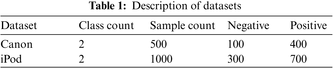
In order to evaluate the performance of the proposed FFL-MLP, the Canon and iPod datasets are used. Table 1 contains information about the dataset. The Canon dataset contains 500 data points, 400 of which are positive cases and 100 of which are negative cases. The iPod dataset contains 1000 examples, 700 of which are positive and 300 of which are negative. Table 2 contains a list of features and their descriptions.

4.1 Analysing Results from a Canon Dataset

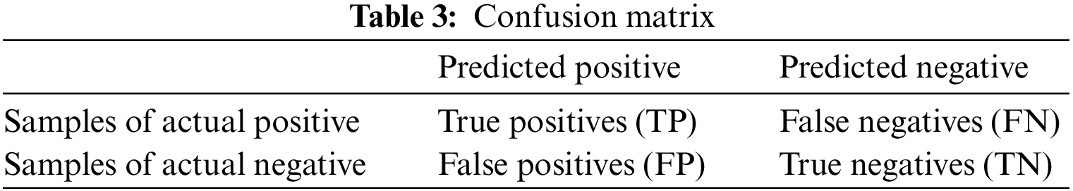
The confusion matrix for the Canon dataset is displayed in Table 3. The table values demonstrate that the 132 instances classified as N and 492 occurrences classed as P in the FFL-MLP are effective in producing results. 491 occurrences are categorized as P and 129 as N by the ACO-K. The ACO assigns P to 486 cases and N to 127 cases in a similar manner. The same approach is also used by PSO to divide the 75 instances into a N class and the 450 instances into a P class. By CSK, 426 cases are categorized as P, whereas 67 are categorized as N. The SVM classifies 56 cases as N cases and 455 cases as P cases.

A comparison of several methodologies employing a variety of validation criteria is shown in Table 4 and Fig. 2. The SVM model, on the other hand, performs less accurately as a classification model, as evidenced by lower sensitivity (95), specificity (89), accuracy (96), and F-score (93). The NN model made an effort to offer a more precise classification to that goal. Nevertheless, the classification result was only passable, with an F-score of 94, a sensitivity score of 95, a specificity score of 89, and an accuracy score of 95.

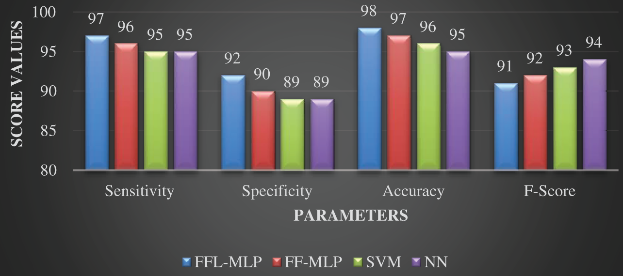
Figure 2: Canon dataset-classifier results

With a maximum accuracy of 97, a specificity of 90, and an F-score of 92, the FFL-MLP model produces a successful classifier outcome.

4.2 Results of iPod Dataset Analysis

According to this dataset, the FF-MLP performs well by classifying 300 cases as N and 700 cases as P. In Table 5 and Fig. 3, the FFL-MLP is compared to the existing method.

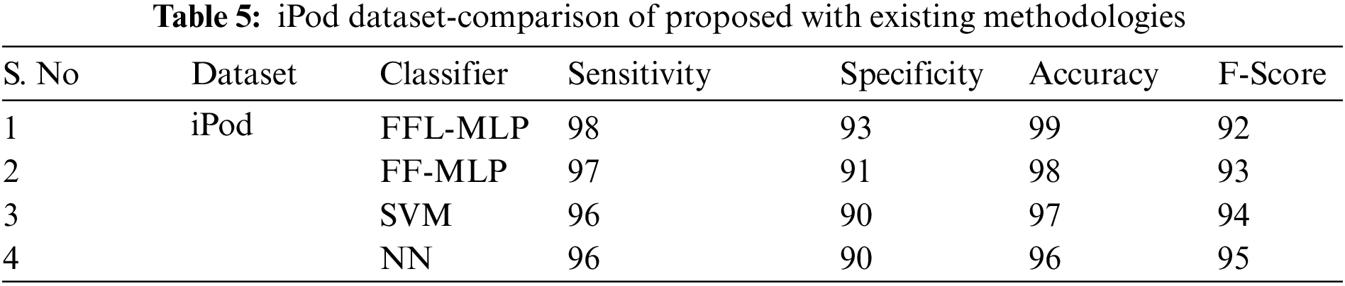
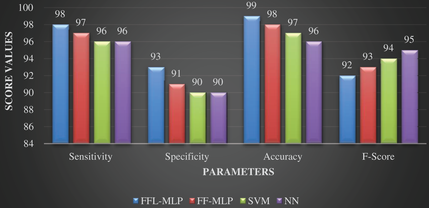
Figure 3: iPod dataset-classifier results

On the iPod dataset, a variety of methods are tested. An examination reveals that the NN classification model is a subpar model, with the overall F-score of 95, lowest specificity of 90, the best accuracy of 96, and a lowest F-score of 95. Having 96% sensitivity, 90% specificity, 97% accuracy, and an F-score of 94, the SVM model likewise performs poorly as a classification model. An acceptable FFL-MLP classification outcome was obtained, with a F-score of 72, specificity of 93, and an accuracy of 99. The specificity, accuracy, F-score, and sensitivity of the FF-MLP model, which offers a moderate classification over earlier methods, are all 97, 91, 98, and 93 respectively.

5  Conclusion

This article devises a new FS-based classification approach to examine sentiments exist in the online product reviews. The FF-MLP method for SA that has been described includes the pre-process of online product reviews to weed out extraneous information, feature extraction, feature selection using FF, and MLP based classification. The FF model is used for extracting attributes from online reviews of product, while MLP is used to classify sentiment. Two datasets are used for the experiment, and a number of assessment criteria are used to gauge the success of the study. With 99% accuracy across a wide range of performance criteria, our FFL-MLP model surpasses its rivals. Hyper-parameter tinkering methods could be used in the future to enhance the FFL-MLP model's output.

Funding Statement: The authors received no specific funding for this study.

Conflicts of Interest: The authors declare that they have no conflicts of interest to report regarding the present study.

References

1. P. Bo and L. Lilliam, “Opinion mining and sentiment analysis,” Foundations and Trends in Information Retrieval, vol. 2, no. 2, pp. 1–13, 2008. [Google Scholar]
2. K. Akshi and M. S. Teeja, “Sentiment analysis: A perspective on its past, present and future,” International Journal of Intelligent Systems and Applications, vol. 4, no. 10, pp. 23–31, 2012. [Google Scholar]
3. Y. Yiming and O. P. Jan, “A comparative study on feature selection in text categorization,” ACM Computing Machine, vol. 2, no. 3, pp. 12–25, 1997. [Google Scholar]
4. M. Carlos, A. Fonseca and F. J. Peter, “An overview of evolutionary algorithms in multi-objective optimization,” Massachusetts Institute of Technology, vol. 3, no. 1, pp. 1–16, 1995. [Google Scholar]
5. R. Sangita, B. Samir and S. C. Sheli, “Nature-inspired swarm intelligence and its applications,” International Journal of Modern Education and Computer Science, vol. 12, no. 4, pp. 55–65, 2014. [Google Scholar]
6. S. Ekbal, A. Saha and C. S. Garbe, “Feature selection using multi-objective optimization for named entity recognition,” International Journal of Pattern Recognition, vol. 2, no. 1, pp. 1937–1940, 2010. [Google Scholar]
7. L. G. William, D. F. Gary and R. John, “Global optimization of statistical functions with simulated annealing,” Journal of Econometrics, vol. 60, no. 2, pp. 65–99, 1994. [Google Scholar]
8. H. A. Mehdi, G. A. Nasser and E. B. Mohammad, “Text feature selection using ant colony optimization,” Expert Systems with Applications, vol. 36, no. 2, pp. 6843–6853, 2009. [Google Scholar]
9. S. Y. Xin, “Firefly algorithm, stochastic test functions and design optimisation,” International Journal of Bio-Inspired Computation, vol. 2, no. 2, pp. 78–84, 2010. [Google Scholar]
10. I. Smeureanu and M. Zurini, “Spam filtering for optimization in internet promotions using bayesian analysis,” Journal of Applied Quantitative Methods, vol. 5, no. 2, pp. 23–34, 2010. [Google Scholar]
11. H. Wang, D. Can, A. Kazemzadeh, F. Bar and S. Narayanan, “A system for real-time twitter sentiment analysis,” Computational Linguistics, vol. 3, no. 2, pp. 115–120, 2012. [Google Scholar]
12. P. Goncalves, B. Fabrício, A. Matheus and C. Meeyoung, “Comparing and combining sentiment analysis methods categories and subject descriptors,” ACM Journal of Networks, vol. 3, no. 5, pp. 27–38, 2013. [Google Scholar]
13. B. Pang, L. Lee and S. Vaithyanathan, “Thumbs up: Sentiment classification using machine learning techniques,” Empirical Methods in Natural Language, vol. 3, no. 4, pp. 79–86, 2002. [Google Scholar]
14. S. J. M. Modha, S. Jalaj and P. S. Gayatri, “Automatic sentiment analysis for unstructured data,” International Journal of Advanced Research in Computer Science, vol. 3, no. 12, pp. 91–97, 2013. [Google Scholar]
15. M. Ahmad, S. Aftab, S. S. Muhammad and U. Waheed, “Tools and techniques for lexicon driven sentiment analysis: A review,” International Journal of Multidisciplinary Sciences and Engineering, vol. 8, no. 1, pp. 17–23, 2017. [Google Scholar]
16. K. Mouthami, K. N. Devi and V. M. Bhaskaran, “Sentiment analysis and classification based on textual reviews,” Computer & Communication, vol. 5, no. 2, pp. 271–276, 2013. [Google Scholar]
17. K. N. Devi and V. M. Bhaskarn, “Online forums hotspot prediction based on sentiment analysis,” Journal of Computational Science, vol. 8, no. 8, pp. 1219–1224, 2012. [Google Scholar]
18. P. S. Earle, D. C. Bowden and M. Guy, “Twitter earthquake detection: Earthquake monitoring in a social world,” Annals of Geophysics, vol. 54, no. 6, pp. 708–715, 2011. [Google Scholar]
19. M. Cheong and V. C. S. Lee, “A microblogging-based approach to terrorism informatics: Exploration and chronicling civilian sentiment and response to terrorism events via twitter,” Information Systems Frontiers, vol. 13, no. 1, pp. 45–59, 2011. [Google Scholar]
20. A. Go, R. Bhayani and L. Huang, “Twitter sentiment classification using distant supervision,” Information Systems Frontiers, vol. 150, no. 12, pp. 1–6, 2009. [Google Scholar]
21. B. Pang and L. Lee, “Opinion mining and sentiment analysis,” Foundations and Trends in Information Retrieval, vol. 2, no. 3, pp. 1–135, 2008. [Google Scholar]
22. A. Bifet and E. Frank, “Sentiment knowledge discovery in twitter streaming data,” Computer Science, vol. 6, no. 2, pp. 1–15, 2010. [Google Scholar]
23. L. Breiman, “Random forests,” Machine Learning, vol. 45, no. 1, pp. 5–32, 2001. [Google Scholar]
24. P. K. Singh and M. H. Shahid, “Methodological study of opinion mining and sentiment analysis techniques,” International Journal of Soft Computing, vol. 5, no. 1, pp. 11–21, 2014. [Google Scholar]
25. J. Khairnar and M. Kinikar, “Machine learning algorithms for opinion mining and sentiment classification,” International Journal of Scientific and Research Publication, vol. 3, no. 6, pp. 1–6, 2013. [Google Scholar]
26. T. M. S. Akshi Kumar, A. Kumar and T. M. Sebastian, “Sentiment analysis on twitter,” International Journal of Computing Science and Mathematics, vol. 9, no. 4, pp. 372–378, 2012. [Google Scholar]
27. A. Pak and P. Paroubek, “Twitter as a corpus for sentiment analysis and opinion mining,” International Journal on Language Resources and Evaluation, vol. 1, no. 2, pp. 1320–1326, 2010. [Google Scholar]
28. T. Sumathi, S. Karthik and M. Marikkannan, “Artificial bee colony optimization for feature selection in opinion mining,” Journal of Theoretical and Applied Information Technology, vol. 66, no. 1, pp. 12–21, 2014. [Google Scholar]
29. D. Ruby and S. Megha, “Weighted sentiment analysis using artificial bee colony algorithm,” International Journal of Science and Research, vol. 12, no. 2, pp. 2319–7064, 2022. [Google Scholar]
30. K. G. Deepak, S. R. Kandula, A. Shweta and E. Asif, “PSO-a sent: Feature selection using particle swarm optimization for aspect-based sentiment analysis,” Natural Language Processing and Information Systems, vol. 2, no. 2, pp. 220–233, 2022. [Google Scholar]
31. Z. Long, S. Linlin and W. Jianhua, “Optimal feature selection using distance-based discrete firefly algorithm with mutual information criterion,” Neural Computing and Applications, vol. 12, no. 2, pp. 1–12, 2016. [Google Scholar]
32. A. Nadhirah, “A review of firefly algorithm,” ARPN Journal of Engineering and Applied Sciences, vol. 9, no. 10, pp. 12–23, 2016. [Google Scholar]
33. W. Bin, “A modified firefly algorithm based on light intensity difference,” Journal of Combinatorial Optimization, vol. 31, no. 3, pp. 1045–1060, 2016. [Google Scholar]
34. W. Sun, X. Chen, X. R. Zhang, G. Z. Dai and P. S. Chang, “A multi-feature learning model with enhanced local attention for vehicle re-identification,” Computers, Materials & Continua, vol. 69, no. 3, pp. 3549–3560, 2021. [Google Scholar]
35. W. Sun, G. C. Zhang, X. R. Zhang, X. Zhang and N. N. Ge, “Fine-grained vehicle type classification using light weight convolutional neural network with feature optimization and joint learning strategy,” Multimedia Tools and Applications, vol. 80, no. 20, pp. 30803–30816, 2021. [Google Scholar]
36. M. M. Iqbal and K. Latha, “An effective community-based link prediction model for improving accuracy in social networks,” Journal of Intelligent and Fuzzy Systems, vol. 42, no. 3, pp. 2695–2711, 2022. [Google Scholar]
37. W. Yanan, W. Jianming, F. Kazuaki, W. Shinya and K. Satoshi, “VAE-based adversarial multimodal domain transfer for video-level sentiment analysis,” IEEE Journal of Cloud Computing, vol. 10, no. 1, pp. 51315– 51324, 2022. [Google Scholar]
38. L. L. Wei, C. H. Chiung and Y. T. Choo, “Sentiment analysis by fusing text and location features of geo-tagged tweets,” IEEE Journal of Cloud Computing, vol. 3, no. 2, pp. 181014–181027, 2020. [Google Scholar]
Cite This Article
Copyright © 2023 The Author(s). Published by Tech Science Press.
This work is licensed under a Creative Commons Attribution 4.0 International License , which permits unrestricted use, distribution, and reproduction in any medium, provided the original work is properly cited.
Downloads
Citation Tools