Artificial Intelligence in Internet of Things System for Predicting Water Quality in Aquaculture Fishponds

1  Introduction

The primary industries in the human food supply chain are the agriculture, animal husbandry, and fishery industries [1,2]. Many Countries have attempted to develop their fishery industries be establishing various fishery types, including capture fisheries and aquaculture fisheries. Aquaculture fisheries are relatively more stable since their production output is easier to plan according to human needs. According to a 2020 report by the Agriculture and Food Agency of the United Nations [3], of the US$401 billion total output value of the global fishery industry in 2018, an output value of US$250 billion had been generated by aquaculture fisheries.

Since Taiwan is surrounded by the sea, fisheries are a major economic industry. According to Fisheries Agency, Council of Agriculture, and Executive Yuan of Taiwan [4], aquaculture fisheries accounted for 44.7% of the total production value (approximately US$1.06 billion), which shows the importance of aquaculture to the overall fishery. The water quality is essential for fish growth and survival [5]. Traditionally, most fishers have judged water quality through visual inspection. Now, some fishers have measured with a dissolved oxygen meter in person at different positions in the pond [6,7]. However, these are inefficient, inaccurate, and dangerous ways. Additionally, the decreasing size of the labor force and increasing labor costs in Taiwan have increased the difficulty of recruiting qualified water quality inspectors who must have experience. As in other technologically advanced countries, therefore, the Taiwan government has promoted the use of artificial intelligence (AI) and internet of things (IoT) technologies in various industries to address these labor issues [8,9]. In the IoT system, a terminal equipped with sensors and other data collection components can collect data and send it to the cloud. Such a terminal can also collect and transmit data to the database of a back-end system through a network or other wireless communication system. Therefore, potential applications of IoT have been discussed in many different domains [10], including transportation logistics [11–13], industrial manufacturing [14–19], and health care [20–25]. In aquaculture, IoT is also used for water quality inspection [26–30]. The above studies demonstrate that integration of AI is a growing trend in industrial applications of IoT.

In smart farming, the IoT can also be used to monitor the growth status of agricultural products. Without further processing and analysis, however, information collected by the IoT has limited practical applications [31]. Therefore, an important emerging technology is the integration of AI in IoT (AIoT) [32], which enables not only monitoring, but also prediction, assessment, and decision-making. That is, AIoT increases efficiency in the management and use of resources and data, which then contributes to cost reduction and trend understanding. Currently, the most common methods of AI are neural networks, deep learning, and machine learning [33]. In farming, IoT is used to detect and collect data from fields [34–38]. In addition, after data collection by IoT, Quiroz et al. [39] applied a convolutional neural network (CNN) to classify the crop. Rezk et al. [40], Rodríguez et al. [41], and Kuo et al. [42] predicted or analyzed the crop yield by using wrapper partial decision tree algorithm (WPART), extreme gradient boosting (XGBoost), and support vector machine (SVM) as well as CNN models, respectively. Hsu et al. [37] not only built a model for predicting yields but also developed a subsystem for detecting unauthorized entry to crop fields.

This study was performed in cooperation with the Industrial Technology Research Institute (ITRI) in Taiwan and a local aquaculture company. The objective was to develop an effective technology that aquaculture practitioners can use to monitor and manage fish farms. The IoT hardware was set up with the assistance of ITRI. In the proposed smart water quality monitoring system, data for crucial factors in the water quality of fishponds were collected by sensors then entered in an intelligent model developed by AI for use in building a smart water quality monitoring system for fishponds.

In the current study, Taguchi method [43] was used to explore and optimize hyperparameter combinations for the prediction models. Orthogonal arrays were used to plan each experiment, to perform each experiment using different hyperparameter combinations, and to record the experimental results. Finally, a response table was used to infer the optimal combination by comparing experimental results among different parameter combinations in the orthogonal array. Then the experiment was performed using the optimal combination. If the experimental result of the optimal combination from the response table was better than all the experimental results in the orthogonal array, it was selected as the hyperparameter architecture. Otherwise, the combination with the optimal result in the orthogonal array was selected. In addition to discussing the model hyperparameters, this research also compared the five-layer and seven-layer LSTM and GRU to find the most suitable model for solving the problem considered in this study. The comparison results indicated that the most applicable model was a seven-layer GRU, which achieved a MAPE of 3.7134%, an RMSE of 0.0638, and an R-value of 0.9984. This model performs better than the model built from the orthogonal array in this study. The GRU enables the water quality monitoring and decision-making system to determine when the oxygenation equipment and the paddlewheel aerator should be started to maintain the quality of the fishpond water, including its dissolved oxygen content (DOC).

According to feedback from the local aquaculture company that participated in this study, the developed system can be used to maintain DOC levels higher than the standard value suitable for farmed fish by activating the oxygenation equipment and the paddlewheel aerator whenever the DOC of the water is insufficient. In addition, compared with the traditional inspection method and the paddlewheel aerator activation all day, the developed method can provide an automatic, safe, and energy-saving way to monitor their fishpond. Thus, the experiment confirmed the effectiveness and practicality of the system developed by this research institute.

This paper is organized as follows. The study related works is briefly discussed in Section 2. Section 3 presents the proposed method. Section 4 presents and discusses the case study results. Finally, Section 5 concludes the study.

2  Related works

The water quality monitoring and decision-making system used a backpropagation neural network (BPNN) described previously [44–47]. The current state of water quality will be affected by the previous state of water quality because the water quality cannot plummet or rise at a glance. That is, the factors which influence the water quality are timing sequence [48]. For an ANN, the output of a single hidden layer is only predicted based on the current data. The prediction results between different hidden layers will not affect each other. ANN must have memory capability to analyze the correlation and sequential data for factors by ANN. However, the BPNN did not have memory capability, so as could not consider timing sequence data. Therefore, this study used recurrent neural networks (RNNs) [49–51] to model because RNNs consider the timing sequence. And then, for systematic hyperparameter optimization, the Taguchi method [43] was used to find the best hyperparameter combination for model prediction accuracy. In addition to simple RNN, the main structure of the model included long short-term memory (LSTM) [51–53] and gated recurrent units (GRU) [51,54]. Since inferred results are fed back to each neuron in the middle layer, the RNN considers the possible influence of the previous results. However, as the time sequence increases, the problem of gradient vanishing appears. That means the gradient tends to zero even equals zero. When input data can no longer be linked to the results, bias in the re-entered input data gradually increases. The LSTM model and GRU model were developed to solve the vanishing gradient problem. The descriptions of LSTM and GRU in detail are in [52] and [54], respectively.

Hong et al. [55] used an LSTM model to build a time-sequence model for predicting symptoms of Alzheimer disease. Chen [56] used an LSTM model to build a model for predicting nonlinear voltage. In Kumar et al. [57], an LSTM model was used to build a deep learning model for predicting and classifying traffic patterns in smart cities. Zhang et al. [58] proposed an integrated EMD-LSTM model, which used EMD to preprocess data and used LSTM for predicting the water quality of the urban drainage network. Zhang et al. [59] proposed a new data-driven model of water quality prediction based on the LSTM model, which used Complete Ensemble Empirical Modal Decomposition with Adaptive Noise (CEEMDAN) to decompose the water quality data to solve the problem of low prediction accuracy caused by the randomness and large volatility of the measured data. Wu et al. [60] used a multi-layer perceptron neural network to process the missing values and used discrete wavelet transform (DWT) to decompose the water quality data, then used LSTM to predict the water quality of the Jinjiang River in China. Hong et al. [61] developed a method of using the LSTM model to build an accurate weather forecasting model. Song et al. [62] used an LSTM model to build a time-sequence model for predicting sea surface height anomaly (SSHA). However, a limitation of the LSTM model is its numerous internal calculations, which tend to decrease prediction and classification speed. Therefore, recent studies have begun to investigate the use of GRU. For example, Yuan et al. [63] used GRU to diagnose and predict industrial manufacturing errors. Another industrial application proposed by Li et al. [64] is the use of GRU for exploring petroleum conglomerate reservoirs. In Leng et al. [65], the GRU model was used to estimate offshore seabed depth by analyzing satellite images. Zhang et al. [66] used the GRU model for traffic system analysis, i.e., to predict automobile collisions with pedestrians under varying traffic conditions. Xu et al. [67] collected infrared thermal images of polymethyl methacrylate (PMMA), used principal component analysis (PCA) to reduce the dimension of the images, and then used GRU to build a model for detecting defects. Jiang et al. [68] proposed a data-driven Fat, oil, and grease (FOG) content prediction model based on deep learning model GRU for diagnosing sewer blockage and overflow. Ali et al. [69] proposed a set of prediction models based on machine learning, deep learning, and statistics for predicting sea surface temperature (SST) and significant wave height (SWH), where in terms of deep learning, the authors used GRU-DNN model architecture. Chi et al. [48] used a wavelet transform (WT) to denoise and used maximal information coefficient (MIC) to select features, then used GRU to predict the water quality of the dish-shaped lakes in Poyang Lake of Jiangxi Province, China.

The above examples demonstrate the many potential applications of LSTM and GRU, but do not explore which is more suitable. Sutskever et al. [70] noted that hyperparameter selection is a critical step when building a deep learning model. A deep learning model cannot be designed systematically and efficiently if the hyperparameters are randomly selected. Therefore, Chou et al. [71] used experimental design method to find the best hyperparameter combination for a CNN. Ho et al. [72] and Ho et al. [73] also used experimental design method to explore hyperparameter combinations for deep residual network (ResNet) and CNN models. In summary, this paper explored the applicability of LSTM and GRU deep learning models for predicting DOC and used a Taguchi method to optimize hyperparameters.

3  Purposed Methodology

3.1 Environment Configuration

The site of this study was a locally owned and operated fish farm in Linbian, Pingtung, Taiwan. Fig. 1 is a schematic diagram of the fish farm, which was cooperated in this study. Above the fishponds are two to four paddlewheel aerators equipped with dissolved oxygenation equipment to accelerate dissolution of oxygen. Various sensors are installed in the fishponds to monitor water quality and other essential factors. The upper left of the diagram depicts the ecological ponds and the water treatment system, which includes the dissolved oxygenation equipment for treating and purifying the water to increase its DOC and overall quality. Based on the actual location, nursery plants and a computer room are located in the south area of the fish farm. The IoT data are sent to this computer room and to the cloud for use in monitoring water quality.

Figure 1: Schematic diagram of field configuration for the fish farms

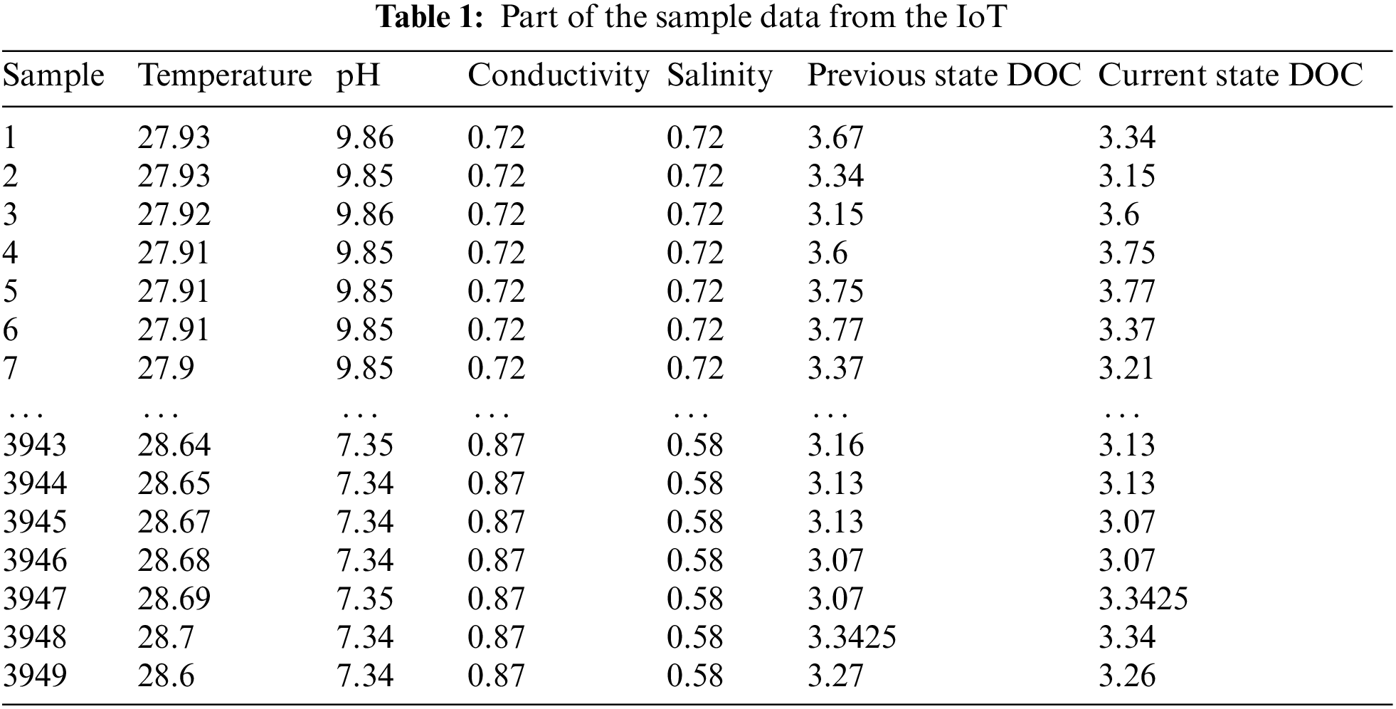
According to Yu et al. [74], Liu et al. [75], Gustilo et al. [76], and the experience of practitioners, DOC (unit: ppm) is a useful metric for water quality because it is affected by conductivity (unit: US/CM), pH, salinity (unit: mg/L), and temperature (unit: °C). Additionally, the previous state DOC has influenced the current state DOC. In this study, based on practitioners’ experience, all five factors (conductivity, pH, salinity, temperature, and previous state DOC) were considered critical factors in the current DOC. However, the weather can indirectly affect these five factors. Therefore, the weather influence also was implied in these five factors. Table 1 shows some data samples, and each data includes conductivity, pH, salinity, temperature, and previous state DOC with the current state DOC. If outliers or nulls exist in the dataset, we used mean imputation to tackle values. Before the modeling, the dataset is normalized and partitioned into 80% train and 20% test data. When model training is complete, the model was verified by the model performance metrics methodology in Section 3.4.

3.2 Configuration of IoT in the Experimental Environment

This study constructed a complete intelligent system for monitoring water quality in fish farms. Fig. 2 shows the system architecture. Data for five critical factors were collected by sensors and transmitted to the computer and data center via a wireless network. The sensor was provided by ITRI, Taiwan, and the sampling time was twenty minutes. Based on these data, the LSTM and GRU models estimated DOC within 20 min. This study also compared performance between the LSTM and GRU. If the system determines that DOC is insufficient after 20 min, it will be automatically triggered to activate the oxygenation equipment and the paddlewheel aerator. In peacetime, the oxygenation equipment always keeps the water with high oxygen and stores it in a water tank. When triggered, the oxygenation equipment will deliver the water with high oxygen into the fishpond. The paddlewheel aerator pumps the oxygen in the air into the water simultaneously. This process will continue until the new predicted DOC value returns to the standard value. According to the experience of practitioners, the standard value of the DOC in the water is three ppm, so if the DOC is lower than three ppm, the oxygenation equipment, and paddlewheel aerator pumps must be activated.

Figure 2: Schematic diagram of IoT configuration

3.3 Modeling Method and its Hyperparameter Optimization

Since current values for critical factors in water quality are dependent on their time series values, BPNN was considered unsuitable for estimating water quality. This study addressed the time series issue by using an RNN model. Under the RNN architecture, the next one input data was influenced by the current feedback value [49,50]. In addition to conventional RNN, common variations of RNN include LSTM [52,53] and GRU [54]. The Taguchi method is a robust experiment method, which can reduce the effect of the cause of variation. Parameter design methods were used for hyperparameter optimization of the LSTM and GRU. To systematically arrange the experiments for training RNN, the Taguchi method [43] was used to search for the optimal hyperparameter combinations for the LSTM and GRU. The Taguchi method was first used to define the number of levels and then to select the appropriate orthogonal table according to the numbers of levels and factors. After selecting appropriate hyperparameters, the L25(56) orthogonal table, shown in Table 2, is used as the experimental design method. To understand the effect of the number of middle layers of LSTM and GRU on performance, the L25(56) orthogonal table has been chosen. Furthermore, according to Srivastava et al. [77], the appropriate addition of dropout layers to the neural networks can reduce the over-fitting problem, so the RNN has at least five layers. If there are more than seven layers, the L125 orthogonal table needs to be selected to double the cost and time of RNN training. Fig. 3 shows that the architecture of the five-layer included an input layer, a middle layer, a dropout layer, a fully connected layer, and an output layer. The key hyperparameters were middle-layer neuron count, maximum iterations, batch size, learning rate, and dropout ratio.

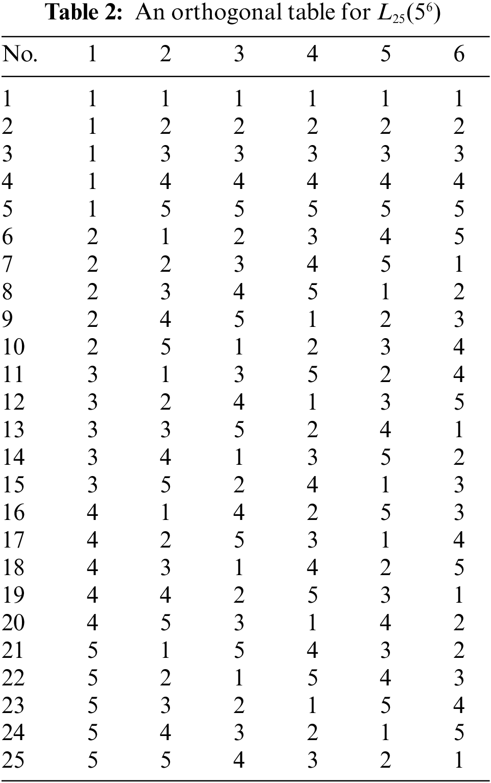
Figure 3: The 5-layer architecture of training model

Fig. 4 shows that the seven-layer included an input layer, a middle layer, a first dropout layer, a second middle layer, a second dropout layer, a fully connected layer, and an output layer. The number of neurons was determined separately for each middle layer, but the dropout ratio of each middle layer was set the same. The number of columns was set according to the number of layers (i.e., five or seven).

Figure 4: The 7-layer architecture of training model

3.3.1 Five-Layer Architecture for Model

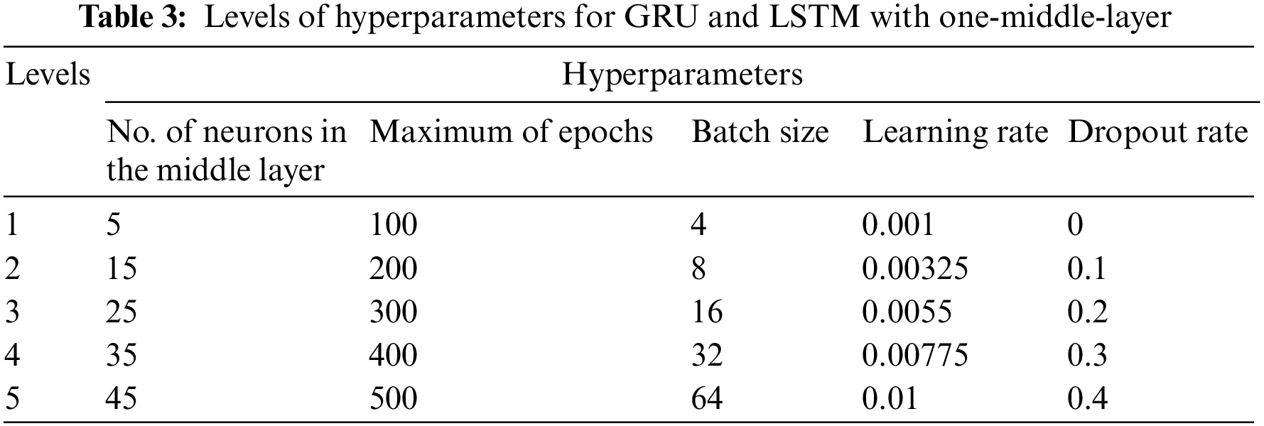
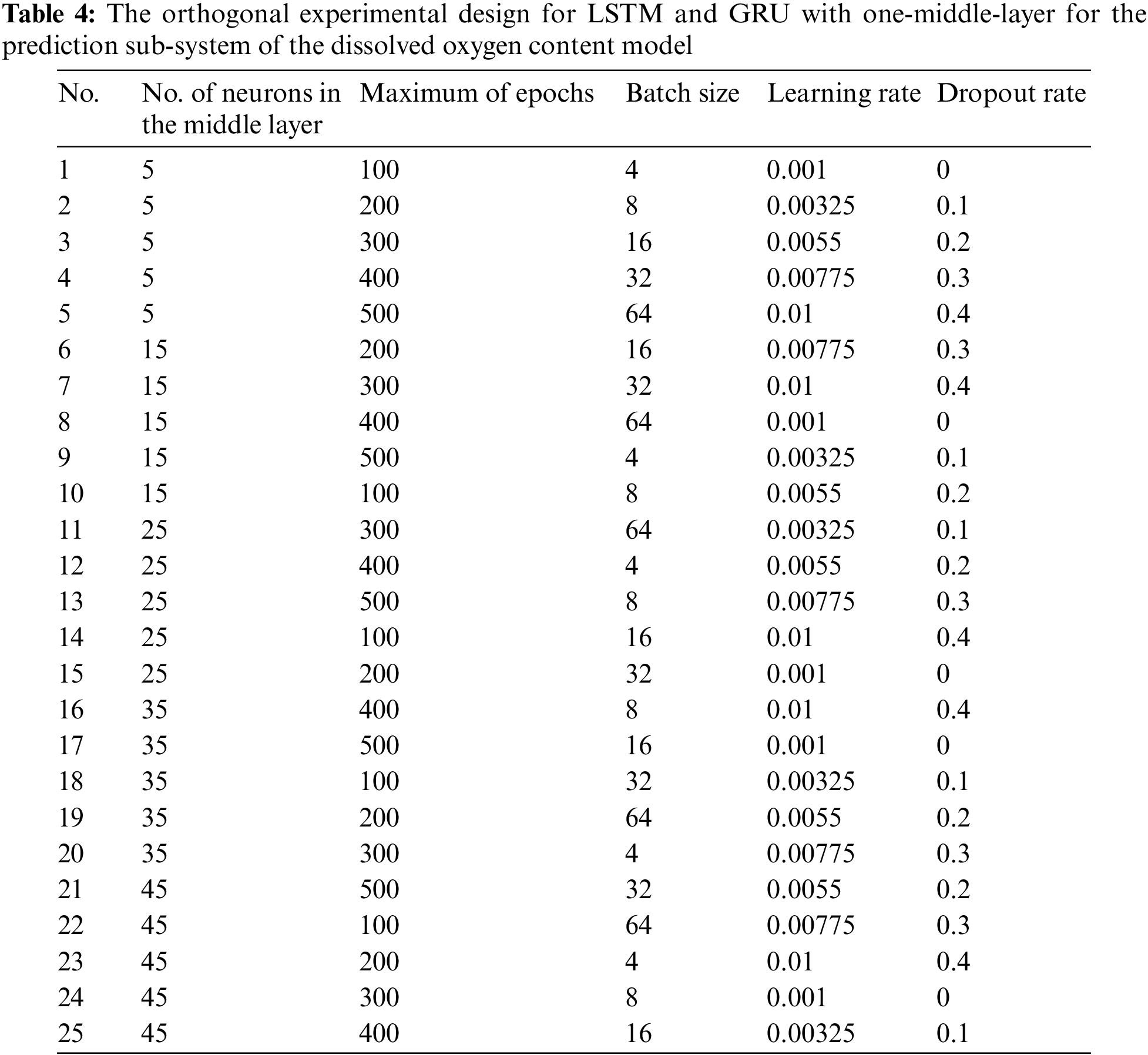
Fig. 3 shows that the five-layer architecture included an input layer, a middle layer, a dropout layer, a fully connected layer, and an output layer. Hyperparameters that needed to be defined were number of middle layer neurons, maximum iterations, batch size, learning rate, and dropout ratio. According to the requirements and level definitions of hyperparameters, the number of levels of each hyperparameter was divided as shown in Table 3. To meet the requirements of the five-layer architecture, the first five columns in Table 4 were used in the experimental configuration. In Table 4, the first column is the middle-layer neuron count, the second column is the maximum iteration count, the third column is batch size, the fourth column is learning rate, and the fifth column is dropout ratio.

3.3.2 Seven-Layer Architecture for Model

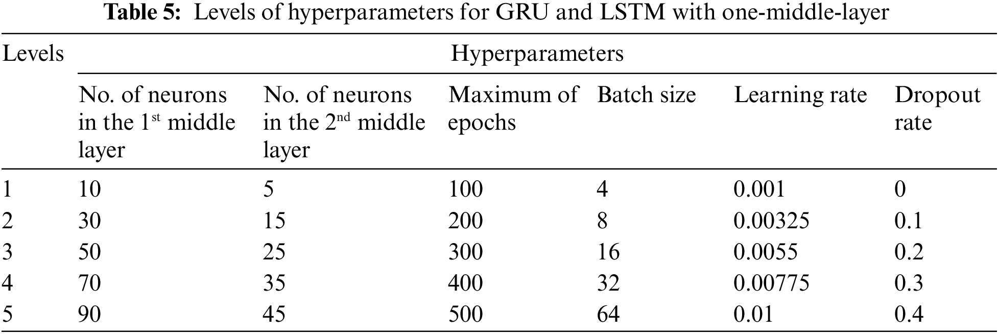
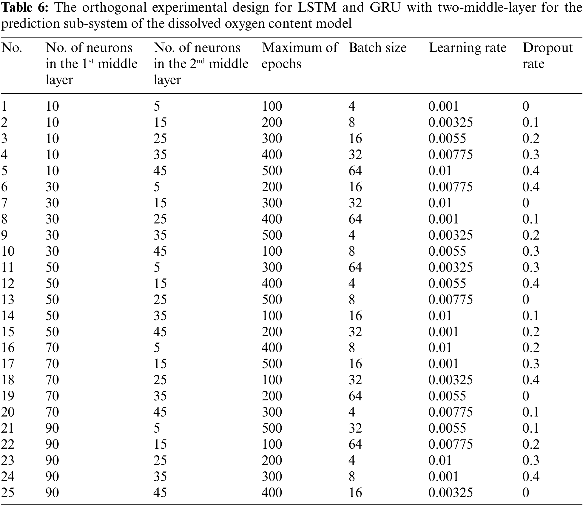
Fig. 4 shows the seven-layer architecture of the model. Compared to the five-layer architecture, the seven-layer model differs in its two middle layers and two dropout layers. In order to discuss this architecture, this study designed hyperparameters for the number of neurons in the two middle layers, the maximum number of iterations, the batch size, the learning rate, and the dropout ratio. Table 5 shows the levels according to the hyperparameter requirements and level definition of the seven-layer architecture. To meet the requirements of the seven-layer architecture, each column in Table 6 was used in a different experimental configuration. In Table 6, the first column is the first middle layer neuron count, the second column is the second middle layer neuron count, the third column is the maximum iteration count, and the fourth column is the batch size. The fifth and the sixth columns are the learning rate and dropout ratio, respectively.

3.4 Model Performance Metric

The applicability of the model proposed in this study was evaluated by calculating root mean square error (RMSE), mean absolute percentage error (MAPE), and correlation coefficient (R-value) [78,79]. In addition, R-squared can calculate by squaring the R-value. When these calculations were performed, every effort was made to ensure the accuracy of test data so that the estimated values would be close to the actual values. The MAPE was the primary value used for model evaluation. The model performance metrics used in this study are described in further detail below:

3.4.1 RMSE

A commonly used model performance metric is RMSE:

RMSE=1n∑i=1n(Fi−Ai)2(1)

In Eq. (1), Fi is the predicted value, and Ai is the actual value. The difference between Fi and Ai is calculated and then the difference is squared. Each value is divided by the number of data items (n), and the square root is used to obtain the RMSE. Generally, RMSE reliably indicates the accuracy of a regression model. However, deviations can deteriorate the accuracy of RMSE during an actual problem-solving task. Therefore, RMSE is a relative index. The accuracy of a prediction model is determined by comparing its RMSE with those of other models.

3.4.2 Correlation Coefficient

Eq. (2) obtains the statistical significance of the correlation coefficient (R-value), which is used to infer the relationship (correlation) between two variables:

R=∑i=1n(Xi−X¯)(Yi−Y¯)∑i=1n(Xi−X¯)2∑i=1n(Yi−Y¯)2(2)

where Xi in the numerator is the actual value, X¯ is the average value of Xi; Yi and are the predicted value and the average value of Yi, respectively. After calculating the individual differences, multiply them, and add up all the multiplied values. The denominator part calculates the square difference separately and then takes the root sign and multiples it. The result will fall between −1 and 1. The closer to −1, the greater the degree of negative correlation. On the contrary, the closer to 1, the greater the degree of positive correlation. The coefficient of determination can be calculated from the correlation coefficient, and the closer the coefficient of determination is to 1, the greater the model's explanatory.

3.4.3 MAPE

Eq. (3) is the calculation for MAPE, which indicates the difference between the predicted value and the corresponding actual value:

MAPE=1n∑i=1n|Fi−AiAi|×100%(3)

In Eq. (3), Ft is the predicted value, and At is the corresponding actual value. The error is divided by the actual value, and the absolute value is obtained. All values are added to the total value, and the average is multiplied by 100%. The MAPE is generally presented as a percentage and has no maximum value. However, a MAPE close to 0% indicates an excellent predictive model, i.e., a model that accurately reflects actual conditions.

4  Results and Discussions

To select the most suitable RNN model, this study explored five-layer architectures and seven-layer architectures in the LSTM and in the GRU as described in the previous section. Taguchi method was used to find the most suitable hyperparameter combination.

4.1 GRU and LSTM Models Based on Five-Layer Architecture

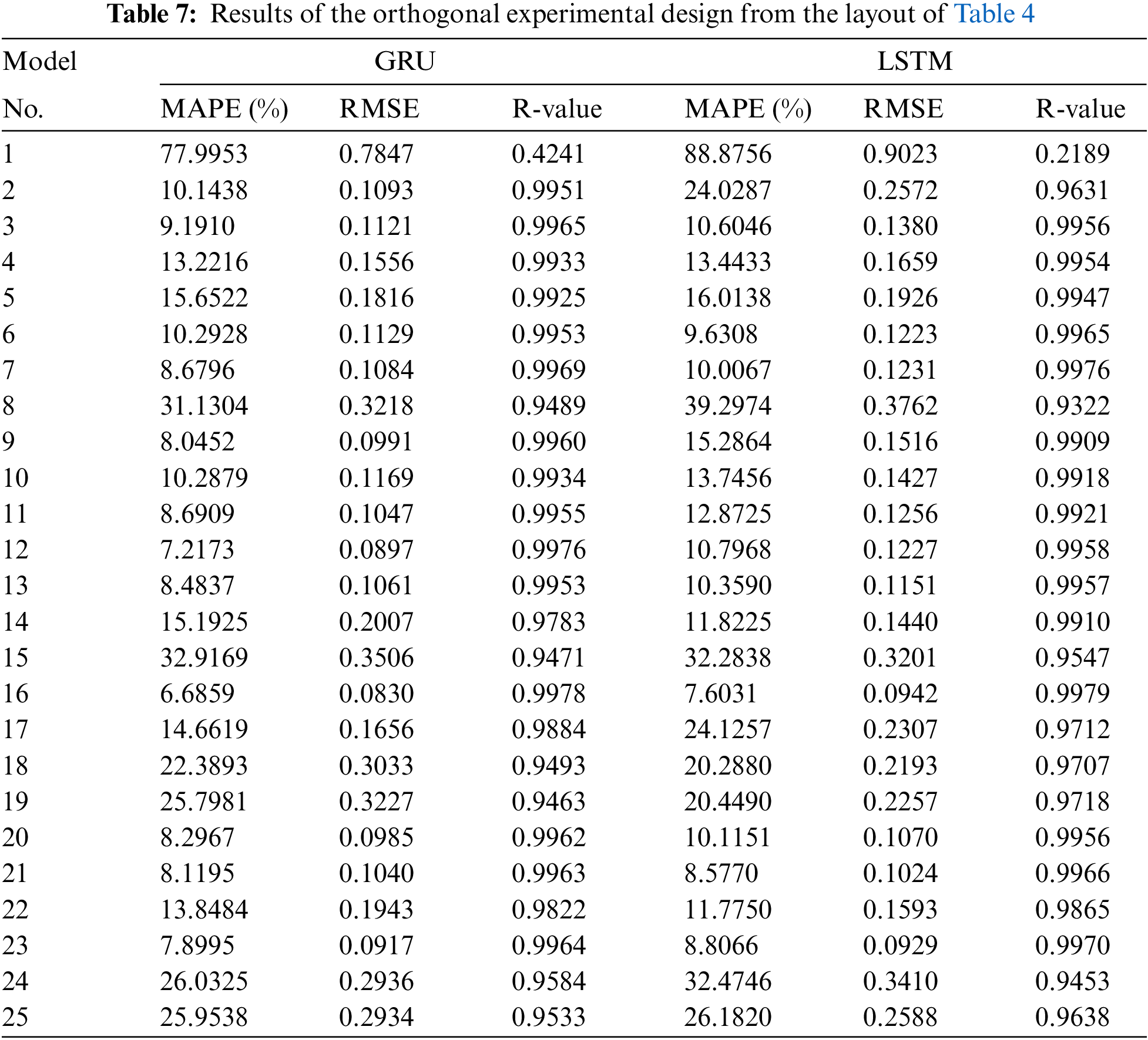
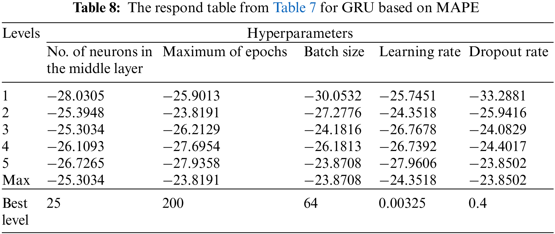
As mentioned in Section 3.3.1, the L25(56) was used to search for the optimal hyperparameter combination. To meet the requirements of the five-layer architecture, the first five columns were selected for the experimental configuration. Each set of experimental configurations was executed ten times, and the results were presented as the average values for MAPE, RMSR, and R-value. Table 7 presents the modeling test results obtained when the experimental configurations in Table 4 were applied to GRU and LSTM. Since the system must use actual data to determine whether the oxygenation equipment and the paddlewheel aerator for DOC must be started, model performance was mainly compared in terms of MAPE. In Table 7, the 16th hyperparameter combination obtained the best results for GRU and LSTM (MAPE values of 6.6859% and 7.6031% for GRU and LSTM, respectively). Table 7 also shows GRU outperformed LSTM. Therefore, GRU was selected for use in calculating the optimal hyperparameter combination. Table 8 shows the optimal hyperparameter combination inferred from the response table when Taguchi method was used for hyperparameter optimization. The optimal combination of hyperparameter values was 25, 200, 64, 0.00325, and 0.4 for middle-layer neuron count, maximum epochs, batch size, learning rate, and dropout rate, respectively. Thirty experiments were performed to verify the accuracy of the model. From the average, MAPE is 6.4421% (RMSE is 0.08475, R-value is 0.9973), which is better than all results in Table 7. In addition, the S.D. values of MAPE, RMSE, and R-value were 0.4676%, 0.0052, and 0.00003, respectively. In these 30 models used to verify, the MAPE, the RMSE, and the R-value of the best one were 5.2802%, 0.0699, and 0.9974, respectively.

4.2 GRU and LSTM Models Based on Seven-Layer Architecture

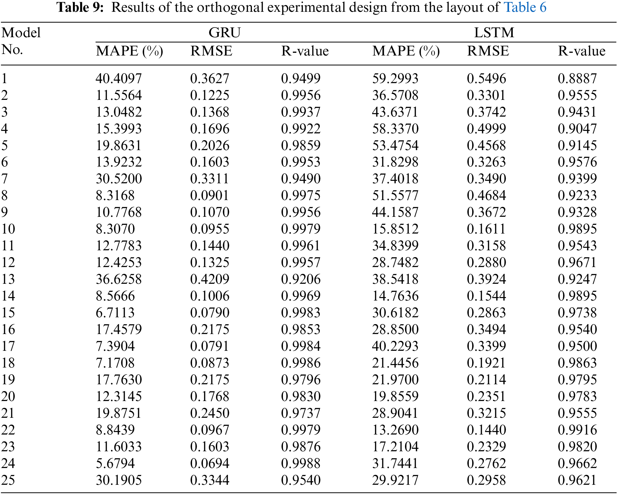
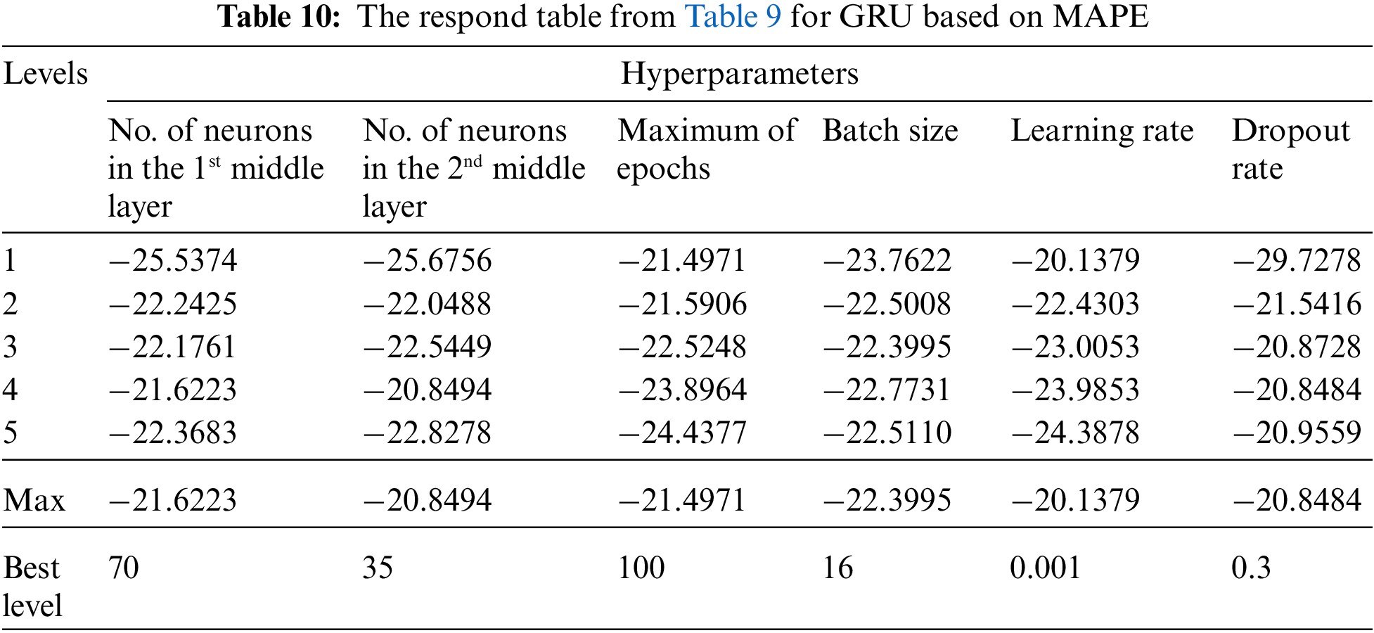
The experimental configuration of the seven-layer architecture is detailed in Section 3.3.2, and L25(56) was used to search for the optimal hyperparameter combination. As in the implementation of the five-layer architecture, each set of experimental configurations was executed ten times, and the average values for MAPE, RMSE, and R-value were again calculated. Table 9 is the modeling test results obtained by executing the L25(56) orthogonal table for the seven-layer architecture. Table 9 shows that GRU performed well when the 24th combination of hyperparameters was used (MAPE 5.6794%) while LSTM performed well when the 22nd group of hyperparameter combinations was used (MAPE 13.2690%). Since the above results confirmed that GRU outperformed LSTM, only the optimal parameter combination for GRU was inferred. Table 10 is the response table inferred from Table 9. Table 10 shows that the optimal values for first middle-layer neuron count, second middle-layer neuron count, maximum epochs, batch size, learning rate, and dropout ratio were 70, 35, 100, 16, 0.001, and 0.3, respectively. When the experiment was repeated 30 times based on this set of optimal values, the average values were MAPE 5.0410%, RMSE 0.0726, and R-value 0.9983; the S.D. values of MAPE, RMSE, and R-value were 0.4676%, 0.0052, and 0.00003, respectively. The average values for MAPE, RMSE, and R-value were superior to the best values in Table 9. In these 30 established models, the MAPE, the RMSE, and the R-value of the best one were 3.7134%, 0.0638, and 0.9984, respectively.

4.3 Comparison and Discussion

Since the seven-layer architecture outperformed the five-layer architecture in terms of MAPE, RMSE, and R-value, the optimal hyperparameter combination calculated by the seven-layer architecture was used to determine the best model. In the best model, which was selected from 30 established GRU models based on seven-layer architecture, the MAPE, the RMSE, and the R-value were 3.7134%; 0.0638; and 0.9984, respectively. Because this paper focuses on the predicted value of DOC, the MAPE is the primary evaluation indicator. If the MAPE is less than 10%, that means the model is excellent [80]. The results show that the proposed method’s best model achieves this requirement. In addition, the seven-layer architecture requires only 25 experiments for optimizing the hyperparameters using Taguchi’s method. The number of experiments required is the same as that of the five-layer architecture.

Furthermore, the models obtained in this study have the best values in terms of RMSE and R-value compared with others. In RMSE, the smaller, the better. The R-value is the opposite of RMSE. In terms of the R-value, the larger, the better. Therefore, this model is an excellent model for DOC prediction.

5  Conclusions

This study was to construct a complete set of intelligent systems for monitoring and predicting fishpond water quality. This system integrated an IoT system and AI method to obtain an AIoT system for DOC predictions and activate the oxygenation equipment and the paddlewheel aerator when DOC in fish pond water is insufficient. The experimental results indicated that the prediction performance of the seven-layer GRU was superior to others. In the model construction process, the Taguchi method was used to rapidly and systematically obtain a brilliant model. The model is excellent from this evaluation result in terms of MAPE, RMSE, and R-value. This system cooperated with the Taiwan ITRI and a local Taiwan aquaculture company to develop. The participating aquaculture company confirmed the effectiveness of the developed system for controlling the DOC of fishpond water. As a practical matter, since the system can rapidly (within 20 min) determine DOC, it provides operators with sufficient time to re-establish the appropriate DOC of fishpond water by activating the oxygenation equipment and the paddlewheel aerator.

Since the current work only considers the DOC of the previous state and up to seven layers of the model. If the hardware and training time of the model allows, we can consider more DOCs of the previous states and higher levels of the neural network.

Acknowledgement: This work was supported in part by the Ministry of Science and Technology, Taiwan, under Grant Numbers MOST 110-2221-E-153-010 and in part by the National Pingtung University under Artificial Intelligence Research Project.

Funding Statement: Publication costs are funded by the Ministry of Science and Technology, Taiwan, under Grant Numbers MOST 110-2221-E-153-010.

Conflicts of Interest: The authors declare that they have no conflicts of interest to report regarding the present study.

References

1. S. N. Chand, Dictionary of Economics. New Delhi, India: Atlantic Publishers & Dist, 2006. [Google Scholar]

2. P. H. Collin, Dictionary of Economics: Over 3000 Terms Clearly Defined. London, UK: Bloomsbury Publishing, 2015. [Google Scholar]

3. FAO, The State of World Fisheries and Aquaculture 2020. Rome, Italy: FAO, 2020. [Google Scholar]

4. Fisheries Agency, Council of Agriculture and Executive Yuan of Taiwan, Fisheries Statistical Yearbook Taiwan, Kinmen and Matau Area 2020. Taipei, Taiwan: Fisheries Agency, Council of Agriculture, Executive Yuan, 2021. [Google Scholar]

5. P. G. Arepalli, M. Akula, R. S. Kalli, A. Kolli, V. P. Popuri et al., “Water quality prediction for salmon fish using gated recurrent unit (GRU) model,” in 2022 Second Int. Conf. on Computer Science, Engineering and Applications (ICCSEA), Gunupur, Odisha, India, pp. 1–5, 2022. [Google Scholar]

6. D. Han, Z. Hu, D. Li and R. Tang, “Nitrogen removal of water and sediment in grass carp aquaculture ponds by mixed nitrifying and denitrifying bacteria and its effects on bacterial community,” Water, vol. 14, no. 12, Art no. 1855, 2022. [Google Scholar]

7. B. Li, R. Jia, Y. Hou, C. Zhang, J. Zhu et al., “The sustainable treatment effect of constructed wetland for the aquaculture effluents from blunt snout bream (megalobrama amblycephala) farm,” Water, vol. 13, no. 23, Art no. 3418, 2021. [Google Scholar]

8. Board of Science and Technology, “Taiwan productivity 4.0 initiative,” Taiwan Economic Forum, vol. 13, no. 3, pp. 47–62, 2015. [Google Scholar]

9. T. Ferry, “The 5+2 industrial innovation plan,” Taiwan Business Topics, vol. 47, no. 5, pp. 15–26, 2017. [Google Scholar]

10. D. Gopal, X. -Z. Gao and J. A. Alzubi, “IoT and big data impact on various engineering applications,” Recent Patents on Engineering, vol. 15, no. 2, pp. 119–120, 2021. [Google Scholar]

11. Z. Gao, D. Wang and H. Zhou, “Intelligent circulation system modeling using bilateral matching theory under internet of things technology,” The Journal of Supercomputing, vol. 77, no. 11, pp. 13514–13531, 2021. [Google Scholar]

12. S. Paiva, M. A. Ahad, G. Tripathi, N. Feroz and G. Casalino, “Enabling technologies for urban smart mobility: Recent trends, opportunities and challenges,” Sensors, vol. 21, no. 6, Art no. 2143, 2021. [Google Scholar]

13. Q. Yuan, Z. Hua and B. Shen, “An automated system of emissions permit trading for transportation firms,” Transportation Research Part E: Logistics and Transportation Review, vol. 152, Art no. 102385, 2021. [Google Scholar]

14. A. Kusiak, “Smart manufacturing,” International Journal of Production Research, vol. 56, no. 1–2, pp. 508–517, 2018. [Google Scholar]

15. F. Tao, Q. Qi, A. Liu and A. Kusiak, “Data-driven smart manufacturing,” Journal of Manufacturing Systems, vol. 48, no. 25, pp. 157–169, 2018. [Google Scholar]

16. H. S. Sim, “A study on the development and effect of smart manufacturing system in PCB line,” Journal of Information Processing Systems, vol. 15, no. 1, pp. 181–188, 2019. [Google Scholar]

17. G. Jadoon, I. Ud Din, A. Almogren and H. Almajed, “Smart and agile manufacturing framework, a case study for automotive industry,” Energies, vol. 13, no. 21, Art no. 5766, 2020. [Google Scholar]

18. M. Calì, “Smart manufacturing technology,” Applied Sciences, vol. 11, no. 17, Art no. 8202, 2021. [Google Scholar]

19. S. Lee, S. H. Rho, S. Lee, J. Lee, S. W. Lee et al., “Implementation of an automated manufacturing process for smart clothing: The case study of a smart sports bra,” Processes, vol. 9, no. 2, Art no. 289, 2021. [Google Scholar]

20. L. Wang, Z. Lou, K. Jiang and G. Shen, “Bio-multifunctional smart wearable sensors for medical devices,” Advanced Intelligent Systems, vol. 1, no. 5, Art no. 1900040, 2019. [Google Scholar]

21. M. Ye, H. Zhang and L. Li, “Research on data mining application of orthopedic rehabilitation information for smart medical,” IEEE Access, vol. 7, pp. 177137–177147, 2019. [Google Scholar]

22. Q. Zhang, C. Bai, Z. Liu, L. T. Yang, H. Yu et al., “A gpu-based residual network for medical image classification in smart medicine,” Information Sciences, vol. 536, no. 5, pp. 91–100, 2020. [Google Scholar]

23. F. Alshehri and G. Muhammad, “A comprehensive survey of the internet of things (IoT) and AI-based smart healthcare,” IEEE Access, vol. 9, pp. 3660–3678, 2021. [Google Scholar]

24. S. C. Sethuraman, P. Kompally, S. P. Mohanty and U. Choppali, “Mywear: A novel smart garment for automatic continuous vital monitoring,” IEEE Transactions on Consumer Electronics, vol. 67, no. 3, pp. 214–222, 2021. [Google Scholar]

25. C. Zhou, J. Hu and N. Chen, “Remote care assistance in emergency department based on smart medical,” Journal of Healthcare Engineering, vol. 2021, Art no. 9971960, 2021. [Google Scholar]

26. M. Manoj, V. Dhilip Kumar, M. Arif, E. -R. Bulai, P. Bulai et al., “State of the art techniques for water quality monitoring systems for fish ponds using IoT and underwater sensors: A review,” Sensors, vol. 22, no. 6, pp. 2088, 2022. [Google Scholar] [PubMed]

27. F. Darmalim, A. A. Hidayat, T. W. Cenggoro, K. Purwandari, S. Darmalim et al., “An integrated system of mobile application and IoT solution for pond monitoring,” IOP Conference Series: Earth and Environmental Science, vol. 794, no. 1, Art no. 012106, 2021. [Google Scholar]

28. R. Ismail, K. Shafinah and K. Latif, “A proposed model of fishpond water quality measurement and monitoring system based on internet of things (IoT),” IOP Conference Series: Earth and Environmental Science, vol. 494, no. 1, pp. 012016, 2020. [Google Scholar]

29. Y. Li, Z. Xie, C. Mo, Y. Chen and J. Wang, “A low-power water quality monitoring system and prediction model,” in 2022 IEEE 24th Int. Workshop on Multimedia Signal Processing (MMSP), Shanghai, China, pp. 1–11, 2022. [Google Scholar]

30. K. -L. Tsai, L. -W. Chen, L. -J. Yang, H. -J. Shiu and H. -W. Chen, “IoT based smart aquaculture system with automatic aerating and water quality monitoring,” Journal of Internet Technology, vol. 23, no. 1, pp. 177–184, 2022. [Google Scholar]

31. S. K. Punia, M. Kumar, T. Stephan, G. G. Deverajan and R. Patan, “Performance analysis of machine learning algorithms for big data classification: Ml and ai-based algorithms for big data analysis,” International Journal of E-Health and Medical Communications (IJEHMC), vol. 12, no. 4, pp. 60–75, 2021. [Google Scholar]

32. A. Ghosh, D. Chakraborty and A. Law, “Artificial intelligence in internet of things,” CAAI Transactions on Intelligence Technology, vol. 3, no. 4, pp. 208–218, 2018. [Google Scholar]

33. S. Russell and P. Norvig, Artificial Intelligence: A Modern Approach, Fourth ed., Upper Saddle River, New Jersey, US: Pearson FT Press, 2020. [Google Scholar]

34. G. Codeluppi, A. Cilfone, L. Davoli and G. Ferrari, “Lorafarm: A lorawan-based smart farming modular IoT architecture,” Sensors, vol. 20, no. 7, Art no. 2028, 2020. [Google Scholar] [PubMed]

35. J. Sanghavi, R. Damdoo and K. Kalyani, “Agribot: IoT based farmbot for smart farming,” Bioscience Biotechnology Research Communications, vol. 13, no. 14, pp. 86–89, 2020. [Google Scholar]

36. G. Adamides, N. Kalatzis, A. Stylianou, N. Marianos, F. Chatzipapadopoulos et al., “Smart farming techniques for climate change adaptation in cyprus,” Atmosphere, vol. 11, no. 6, Art no. 557, 2020. [Google Scholar]

37. W. -L. Hsu, W. -K. Wang, W. -H. Fan, Y. -C. Shiau, M. -L. Yang et al., “Application of internet of things in smart farm watering system,” Sensors and Materials, vol. 33, no. 1, pp. 269–283, 2021. [Google Scholar]

38. T. Kassem, I. Shahrour, J. El Khattabi and A. Raslan, “Smart and sustainable aquaculture farms,” Sustainability, vol. 13, no. 19, Art no. 10685, 2021. [Google Scholar]

39. I. A. Quiroz and G. H. Alférez, “Image recognition of legacy blueberries in a chilean smart farm through deep learning,” Computers and Electronics in Agriculture, vol. 168, Art no. 105044, 2020. [Google Scholar]

40. N. G. Rezk, E. E. -D. Hemdan, A. -F. Attia, A. El-Sayed and M. A. El-Rashidy, “An efficient IoT based smart farming system using machine learning algorithms,” Multimedia Tools and Applications, vol. 80, no. 1, pp. 773–797, 2021. [Google Scholar]

41. J. P. Rodríguez, A. I. Montoya-Munoz, C. Rodriguez-Pabon, J. Hoyos and J. C. Corrales, “IoT-agro: A smart farming system to colombian coffee farms,” Computers and Electronics in Agriculture, vol. 190, Art no. 106442, 2021. [Google Scholar]

42. P. -H. Kuo, R. -J. Liou, P. Nilaphruek, K. Kanchanasatian, T. -H. Chen et al., “Multi-sensor-based environmental forecasting system for smart durian farms in tropical regions,” Sensors and Materials, vol. 33, no. 10, pp. 3547–3561, 2021. [Google Scholar]

43. G. I. Taguchi, S. Chowdhury and S. Taguchi, Robust Engineering: Learn How to Boost Quality While Reducing Costs & Time to Market. New York, US: McGraw Hill, 2000. [Google Scholar]

44. R. C. Gustilo, E. P. Dadios, E. Calilung and L. A. G. Lim, “Neuro-fuzzy control techniques for optimal water quality index in a small scale tiger prawn aquaculture setup,” Journal of Advanced Computational Intelligence and Intelligent Informatics, vol. 18, no. 5, pp. 805–811, 2014. [Google Scholar]

45. P. Y. Yang, J. T. Tsai and J. H. Chou, “Prediction analysis of oxygen content in the water for the fish farm in southern taiwan,” in 2017 Int. Conf. on System Science and Engineering (ICSSE), Ho Chi Minh City, Vietnam, pp. 629–631, 2017. [Google Scholar]

46. P. Y. Yang, J. T. Tsai, J. H. Chou, W. H. Ho and Y. Y. Lai, “Prediction of water quality evaluation for fish ponds of aquaculture,” in 2017 56th Annual Conf. of the Society of Instrument and Control Engineers of Japan (SICE), Kanazawa, Japan, Kanazawa University, pp. 545–546, 2017. [Google Scholar]

47. P. Y. Yang, J. H. Chou, J. T. Tsai, Y. Ma and W. H. Ho, “Prediction for dissolved oxygen in water of fish farm by using general regression neural network,” in 2018 IEEE Int. Conf. on Information and Automation (ICIA), Wuyi Mountain, Fujian, China, pp. 1132–1135, 2018. [Google Scholar]

48. D. Chi, Q. Huang and L. Liu, “Dissolved oxygen concentration prediction model based on WT-MIC-GRU—A case study in dish-shaped lakes of poyang lake,” Entropy, vol. 24, no. 4, Art no. 457, 2022. [Google Scholar] [PubMed]

49. A. Robinson and F. Fallside, The Utility Driven Dynamic Error Propagation Network. Cambridge, UK: University of Cambridge Department of Engineering Cambridge, 1987. [Google Scholar]

50. Y. Bengio, P. Simard and P. Frasconi, “Learning long-term dependencies with gradient descent is difficult,” IEEE Transactions on Neural Networks, vol. 5, no. 2, pp. 157–166, 1994. [Google Scholar] [PubMed]

51. K. P. Wai, M. Y. Chia, C. H. Koo, Y. F. Huang and W. C. Chong, “Applications of deep learning in water quality management: A state-of-the-art review,” Journal of Hydrology, vol. 613, Art no. 128332, 2022. [Google Scholar]

52. S. Hochreiter and J. Schmidhuber, “Long short-term memory,” Neural Computation, vol. 9, no. 8, pp. 1735–1780, 1997. [Google Scholar] [PubMed]

53. J. Martens and I. Sutskever, “Learning recurrent neural networks with hessian-free optimization,” in Proc. of the 28th Int. Conf. on Machine Learning (ICML), L. Getoor, T. Scheffer (Eds.Bellevue Washington, USA, 1033–1040, 2011. [Google Scholar]

54. K. Cho, B. Van Merriënboer, C. Gulcehre, D. Bahdanau, F. Bougares et al., “Learning phrase representations using RNN encoder-decoder for statistical machine translation,” arXiv preprint, 2014. [Google Scholar]

55. X. Hong, R. Lin, C. Yang, N. Zeng, C. Cai et al., “Predicting alzheimer’s disease using LSTM,” IEEE Access, vol. 7, pp. 80893–80901, 2019. [Google Scholar]

56. Y. Chen, “Voltages prediction algorithm based on LSTM recurrent neural network,” Optik, vol. 220, Art no. 164869, 2020. [Google Scholar]

57. S. Kumar, A. Damaraju, A. Kumar, S. Kumari and C. -M. Chen, “LSTM network for transportation mode detection,” Journal of Internet Technology, vol. 22, no. 4, pp. 891–902, 2021. [Google Scholar]

58. Y. Zhang, C. Li, Y. Jiang, L. Sun, R. Zhao et al., “Accurate prediction of water quality in urban drainage network with integrated EMD-LSTM model,” Journal of Cleaner Production, vol. 354, Art no. 131724, 2022. [Google Scholar]

59. L. Zhang, Z. Jiang, S. He, J. Duan, P. Wang et al., “Study on water quality prediction of urban reservoir by coupled ceemdan decomposition and LSTM neural network model,” Water Resources Management, vol. 36, no. 10, pp. 3715–3735, 2022. [Google Scholar]

60. J. Wu and Z. Wang, “A hybrid model for water quality prediction based on an artificial neural network, wavelet transform, and long short-term memory,” Water, vol. 14, no. 4, Art no. 610, 2022. [Google Scholar]

61. S. Hong, J. H. Kim, D. S. Choi and K. Baek, “Development of surface weather forecast model by using LSTM machine learning method,” Atmosphere, vol. 31, no. 1, pp. 73–83, 2021. [Google Scholar]

62. T. Song, J. Jiang, W. Li and D. Xu, “A deep learning method with merged LSTM neural networks for SSHA prediction,” IEEE Journal of Selected Topics in Applied Earth Observations and Remote Sensing, vol. 13, pp. 2853–2860, 2020. [Google Scholar]

63. J. Yuan and Y. Tian, “An intelligent fault diagnosis method using GRU neural network towards sequential data in dynamic processes,” Processes, vol. 7, no. 3, pp. 152, 2019. [Google Scholar]

64. X. Li, X. Ma, F. Xiao, F. Wang and S. Zhang, “Application of gated recurrent unit (GRU) neural network for smart batch production prediction,” Energies, vol. 13, no. 22, Art no. 6121, 2020. [Google Scholar]

65. Z. Leng, J. Zhang, Y. Ma and J. Zhang, “Underwater topography inversion in liaodong shoal based on GRU deep learning model,” Remote Sensing, vol. 12, no. 24, Art no. 4068, 2020. [Google Scholar]

66. S. Zhang, M. Abdel-Aty, Y. Wu and O. Zheng, “Modeling pedestrians’ near-accident events at signalized intersections using gated recurrent unit (GRU),” Accident Analysis & Prevention, vol. 148, Art no. 105844, 2020. [Google Scholar]

67. L. Xu and J. Hu, “A method of defect depth recognition in active infrared thermography based on GRU networks,” Applied Sciences, vol. 11, no. 14, Art no. 6387, 2021. [Google Scholar]

68. Y. Jiang, C. Li, Y. Zhang, R. Zhao, K. Yan et al., “Data-driven method based on deep learning algorithm for detecting fat, oil, and grease (FOG) of sewer networks in urban commercial areas,” Water Research, vol. 207, Art no. 117797, 2021. [Google Scholar] [PubMed]

69. A. Ali, A. Fathalla, A. Salah, M. Bekhit and E. Eldesouky, “Marine data prediction: An evaluation of machine learning, deep learning, and statistical predictive models,” Computational Intelligence and Neuroscience, vol. 2021, Art no. 8551167, 2021. [Google Scholar]

70. I. Sutskever, J. Martens, G. Dahl and G. Hinton, “On the importance of initialization and momentum in deep learning,” in Proc. of the 30th Int. Conf. on Machine Learning, Atlanta, Georgia, USA, Proceedings of Machine Learning Research, vol. 28, no. 3, pp. 1139–1147, 2013. [Google Scholar]

71. F. I. Chou, Y. K. Tsai, Y. M. Chen, J. T. Tsai and C. C. Kuo, “Optimizing parameters of multi-layer convolutional neural network by modeling and optimization method,” IEEE Access, vol. 7, pp. 68316–68330, 2019. [Google Scholar]

72. W. -H. Ho, T. -H. Huang, P. -Y. Yang, J. -H. Chou, H. -S. Huang et al., “Artificial intelligence classification model for macular degeneration images: A robust optimization framework for residual neural networks,” BMC Bioinformatics, vol. 22, no. 148, pp. 21, 2021. [Google Scholar]

73. W. -H. Ho, T. -H. Huang, P. -Y. Yang, J. -H. Chou, J. -Y. Qu et al., “Robust optimization of convolutional neural networks with a uniform experiment design method: A case of phonocardiogram testing in patients with heart diseases,” BMC Bioinformatics, vol. 22, no. 5, pp. 345, 2021. [Google Scholar]

74. H. Yu, L. Yang, D. Li and Y. Chen, “A hybrid intelligent soft computing method for ammonia nitrogen prediction in aquaculture,” Information Processing in Agriculture, vol. 8, no. 1, pp. 64–74, 2021. [Google Scholar]

75. S. Liu, L. Xu, Y. Jiang, D. Li, Y. Chen et al., “A hybrid wa-cpso-lssvr model for dissolved oxygen content prediction in crab culture,” Engineering Applications of Artificial Intelligence, vol. 29, no. 4, pp. 114–124, 2014. [Google Scholar]

76. R. C. Gustilo and E. Dadios, “Optimal control of prawn aquaculture water quality index using artificial neural networks,” in 2011 IEEE 5th Int. Conf. on Cybernetics and Intelligent Systems (CIS), Qingdao, China, pp. 266–271, 2011. [Google Scholar]

77. N. Srivastava, G. Hinton, A. Krizhevsky, I. Sutskever and R. Salakhutdinov, “Dropout: A simple way to prevent neural networks from overfitting,” Journal of Machine Learning Research, vol. 15, no. 1, pp. 1929–1958, 2014. [Google Scholar]

78. R. J. Hyndman and A. B. Koehler, “Another look at measures of forecast accuracy,” International Journal of Forecasting, vol. 22, no. 4, pp. 679–688, 2006. [Google Scholar]

79. P. Bobko, Correlation and Regression: Applications for Industrial Organizational Psychology and Management, Second ed., Thousand Oaks, CA, US: Sage Publications, 2001. [Google Scholar]

80. R. J. Chen, P. Bloomfield and J. S. Fu, “An evaluation of alternative forecasting methods to recreation visitation,” Journal of Leisure Research, vol. 35, no. 4, pp. 441–454, 2003. [Google Scholar]