Network Intrusion Detection in Internet of Blended Environment Using Ensemble of Heterogeneous Autoencoders (E-HAE)

1  Introduction

Technology sectors have rapidly converged to provide versatile, high-quality services. For example, to achieve splendid treatment from health care centers, services from a smart grid, smart buildings, and smart healthcare can be aggregated. The smart grid ensures a consistently adequate energy supply through its decentralized energy generation and intelligent self-healing capabilities [1]. Smart buildings, on the other hand, facilitate high-quality services for health professionals and clients, such as providing safe and secure spaces or pleasant and controlled environments [2]. Furthermore, smart healthcare enables smart health monitoring and personalized healthcare services [3]. Consequently, the operations of each sector are becoming highly interdependent and indivisible. For example, the performance of a smart grid is substantially dependent on the effective functioning of smart buildings and vice versa [4,5]. As a result, there is a highly sophisticated interconnection between people, materials, and institutions. This environment in which the Internet of Things (IoT), big data, and AI converge can be collectively referred to as the internet of blended environment (IoBE) to emphasize the mixed and indivisible characteristics of the environment [6].

The convergence of these technologies brings challenging problems, particularly from the cybersecurity perspective, as it introduces a new form of blended threats that exploit the vulnerabilities of weak links as a steppingstone to the most sensitive sectors, such as finance, healthcare, and grid systems. Some of the most common blended threats during the early ages of smart technologies included Code Red, Bugbear, and Nimda [7–9]. For example, attackers were able to steal sensitive information, such as social security numbers and medical records, from Anthem Inc. using a blended threat named Code Red [7]. The number of attack surfaces is increasing exponentially as it is becoming easier for new attack vectors to emerge, following the growing use of IoT technology to connect to corporate networks and cloud-based applications. Such attacks are perilous because of their potential ability to exploit zero-day vulnerabilities. Although the term “blended threat” is often used to refer to an attack that combines multiple techniques and methods, we use it to refer to an attack that exploits multiple vulnerabilities in the IoBE to evade its target. Section 2.3 provides a further explanation of the nature of blended threats.

Having a threat detection and identification system developed by considering such an environment is the primary step that must be taken to mitigate blended threats. Owing to the dynamic and complex nature of the environment, cyberattacks in IoBE have a higher probability of demonstrating solid relationships and mutual effects on each other. Therefore, it is essential to accurately model the subtle temporal and spatial connections between the network traffics generated in IoBE to effectively characterize malicious or anomalous flows in the environment. Machine learning, such as autoencoder and its variants, has shown remarkable achievements, particularly in network intrusion detection [10–13]. Zhang et al. [10] and Yan et al. [11] proposed unsupervised network intrusion detection system (NIDS) by using the stacked autoencoder (SAE) for effective dimensionality reduction. The authors add and leverages the sparsity constraint on the hidden layer of SAE to enhance the generalizability of the proposed approach, particularly for the large-scale intrusion detection systems with massive and high dimensional network traffic. Similarly, Al-Qatf et al. [12] proposed unsupervised NIDS combining the dimensionality reduction power of SAE with the classification potential of Support vector machine. The author achieved a competitive classification result compared to the baseline approaches after applying the proposed NIDS on the NSL-KDD dataset. Similarly, recurrent neural networks and convolutional neural network-based models have shown better performance in accurately modeling both temporal and spatial characteristics [14–16]. Therefore, it has become common to apply a combination of these models and approaches to achieve better performance.

Most of these approaches operate by first training on normal or benign network traffic and then characterizing any deviation as an intrusion or attack. In other words, an anomaly threshold is computed to define a classification boundary between benign and anomalous traffic based on the typical loss exhibited by the model when reconstructing normal network traffic. If insufficiently designed, the models will suffer significantly from a high rate of false alarms, which eventually degrade their performance. Furthermore, the convergence of various heterogeneous environments in the IoBE makes things worse, as it is most likely that the underlying NIDS will experience numerous unmodeled behaviors. To address this problem, we propose a blended threat detection approach considering the possible impact and dimensionality of the new attack surfaces due to the convergence of different technology sectors in the IoBE. The proposed approach encompasses an ensemble of heterogeneous probabilistic autoencoders combining the corresponding advantages of the convolutional variational autoencoder (Conv-VAE) and long short-term memory variational autoencoder (LSTM-VAE). The aggregation of these models intends to effectively characterize the dynamic properties of network traffic and the subtle relationship between the intrinsic nature of blended threats. Furthermore, to address the possible false alarm rate due to heterogeneity in the IoBE data, we propose an ensemble anomaly threshold computing approach based on the individual loss results of both probabilistic models. The optimum anomaly threshold is computed during the training phase, and the most representative probabilistic reconstruction error per traffic is determined during the testing phase. An extensive experiment was conducted on ToN-IoT network intrusion detection datasets, and the results indicated that the proposed solution achieved 96.02% detection accuracy. Furthermore, we conducted a performance comparison against various single model (autoencoder)-based network intrusion detection approaches: autoencoder, variational autoencoder, convolutional variational autoencoder, and long short-term memory variational autoencoder. The results indicated that the proposed model outperformed all other models by demonstrating F1-score improvements of 4.99%, 2.25%, 1.92%, and 3.69%, respectively.

The following points summarize the main contributions of this paper:

•   We provide a network intrusion detection system to detect blended threats in the internet of blended environment (IoBE), considering the possible impact and dimensionality of new attack surfaces resulting from the convergence of different technology sectors.

•   We analyze the dimensionality and impact of blended threats in the IoBE.

•   We provide an optimal anomaly threshold computation approach using an ensemble of heterogeneous autoencoders, in which an optimal anomaly score is computed during the training phase based on the respective loss distribution of each autoencoders, and the most representative probabilistic reconstruction error per traffic is determined adaptively during the test phase.

•   Our approach demonstrated 3.99%, 1.95%, 1.92%, and 2.69% F1-score improvements compared to the single autoencoder-based network intrusion detection systems: autoencoder, variational autoencoder, convolutional variational autoencoder, and long-short term memory autoencoder, respectively.

The remainder of this paper is structured as follows: in Section 2, we review some background information needed to adequately understand the proposed solution; in Section 3, we analyze the dimensionality and impact of blended threats in the IoBE; in Section 4, we discuss the proposed method in detail, including the problem formulation and model construction; in Section 5, we discuss the implementation of the proposed approach, elaborating on the experimental setting and data preprocessing; in Section 6, we evaluate and discuss the overall performance of our proposed technique; and finally, we provide concluding remarks in Section 7.

2  Background

This section provides important background information to help better understand the different topics covered in the manuscript. Furthermore, Table 1 provides descriptions of the notations used in the manuscript to denote mathematical expressions.

2.1 Recurrent Neural Network (RNN) and Long Short-Term Memory (LSTM)

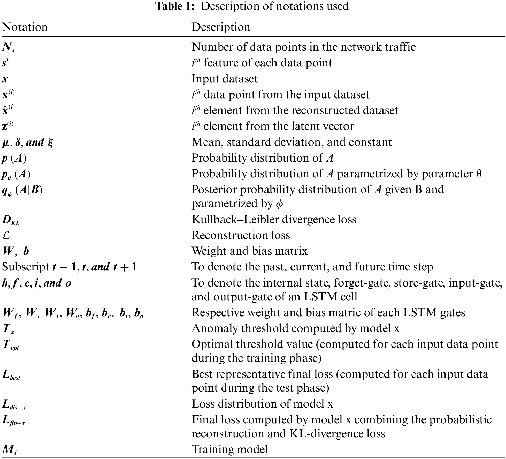
An RNN is a type of deep learning neural network that was primarily developed to model sequences in data when patterns in data change with time [17,18]. In a standard neural network, the information flows only in one direction—from input to output—which prevents the network from maintaining information about previous events when there is a sequence of events in time. In contrast, the simple structure of an RNN has a built-in feedback loop that enables the network to analyze current and future information by allowing the information to persist over time. Similarly, the RNN allows information to flow through time by applying a recurrence relation at every timestep to process a sequence [18]. At some timestep t, unlike the standard neural network, which only computes the output vector yt from the input vector xt, the RNN computes an internal state update ht and passes this information from timestep t to the subsequent timestep t+1. At each timestep t, the internal state ht is updated by applying a function fw that is parametrized by a set of weights w and takes the old state ht−1 and an input vector xt as arguments, as shown in Eq. (1). Most importantly, the same function with its set of weight parameters is used throughout the entire timestep. The network learns this set of parameters during training, as shown in Fig. 1. Note that learning in a neural network is an iterative process of adjusting the difference between the model output and expected output by computing the model loss, backpropagating, and adjusting the weight parameters to minimize the loss.

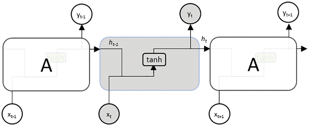
Figure 1: RNN structure

ht=fw(ht−1,xt)(1)

However, in an RNN, unlike a standard neural network, the gradient of the total loss is backpropagated in time to the beginning of the data sequence [18,19]. This results in an exploding gradient problem when the gradients are larger than one, and a vanishing gradient problem when they are less than one. In the latter case, the network is less likely to capture long-term dependencies because of difficulties in propagating the loss further into the distant past. Long short-term memory (LSTM), on the other hand, is a variant of RNN that was explicitly designed to avoid such long-term dependency problems, using the inherent behavior of remembering important information for long periods [19,20]. This is achieved by carefully regulating the information flow and storage using a key structure called a gate, which enables the LSTM to selectively add or remove information to its cell state, as illustrated in Fig. 2.

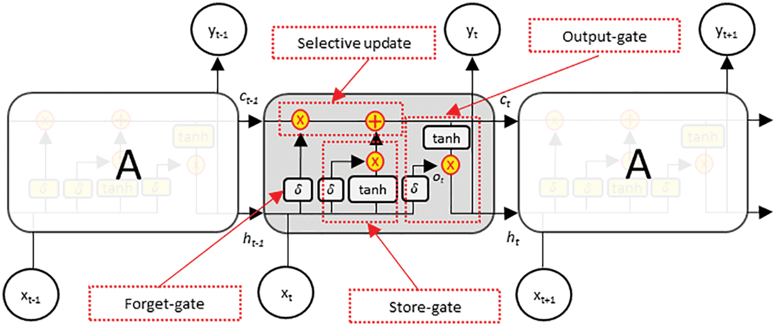
Figure 2: LSTM structure

In general, information passing through a single layer of LSTM involves four major steps: forgetting irrelevant history, storing the relevant part of the new information, selectively updating the internal state based on what to forget and what to store, and finally generating an output, as shown in Fig. 2. In the first step, the LSTM decides on part of the information to be forgotten using the function ft composed of the prior internal state ht−1 and the current input xt, as shown in Eq. (5). The second step is to determine the relevancy of the new information candidate Ct, by adding stored portion of the previous cell state (ft∗Ct−1) and portion of the current cell state to be used (it∗ ′Ct), as shown in Eq. (2). The cell state is then selectively updated in the third step, taking the relevant part of both the prior and current information, as shown in Eq. (4). Finally, the output gate provides an output to the next timestep, deciding on part of the information encoded in the cell state using the sigmoid layer, as shown in Eq. (3). A combination of these steps helps each LSTM layer to create and maintain an internal independent cell state, which allows the uninterrupted flow of the gradient through time.

Ct=ft∗Ct−1+it∗ ′Ct(2)

Ot=δ(w0.[ht−1,xt]+b0)(3)

ht=Ot∗tanh⁡(Ct)(4)

ft=δ(Wf.(ht−1,xt)+bf)={0,forget everything1,remeber everything(5)

where xt is the input to the current timestep, Wf is the weight matrix, bf is the bias, and ht−1 is the hidden state of the previous timestep.

2.2 Autoencoder and Variational Autoencoder

Autoencoders are simple generative models designed to automatically learn low-dimensional feature representations of data by understanding the underlying hidden structure [21,22,11]. They are composed of a concatenated encoder and decoder block, as shown in Fig. 3a, where the encoder block maps the input space x into a low-dimensional representation vector (latent space) z, and the decoder block reconstructs the original input space x by mapping the latent space vector z back to the dimensionality of the input space x. The network is trained to learn the latent vector z using an unsupervised approach by minimizing the reconstruction loss, that is, the difference between the original input space and the reconstructed input space and generating an output that resembles the input space as accurately as possible.

Figure 3: Structure of (a) autoencoder and (b) variational autoencoder

However, the standard autoencoder follows a deterministic encoding approach that enforces the input space into a deterministic latent vector, presenting the latent space as a bottleneck in the network. This implies that the quality of the autoencoders mostly depends on determining the appropriate dimensionality of the latent space. The higher the dimensionality, the poorer the encoding functionality, and the lower the dimensionality, the poorer the quality of the reconstructed output [22]. In contrast, the variational autoencoder (VAE) is a variant of a generative model designed to avoid the bottleneck problem in the standard autoencoder by replacing the deterministic latent-space learning operation with a probabilistic sampling operation [21,23]. In other words, instead of learning the latent variable directly from the encoder operation, the VAE learns the mean (μ) and variance (δ) that parametrize a probability distribution for latent variables in the latent vector. The probabilistic representation of the latent space is then sampled from the means and variances of the described distribution. Both the encoder and decoder in the VAE have a probabilistic nature, in which the encoder computes pϕ(z|x), the probability distribution of the latent vector z given the input space x, and the decoder computes the reverse operation qθ(x˙|z), the probability distribution of the reconstructed input space x˙ given the latent vector z. In addition to the reconstruction loss in the standard autoencoders, to minimize the overfitting problem, the loss function ℒ of the VAE, as shown in Eq. (6), contains a regularization term that imposes a constraint on learning the latent distribution by placing a prior p(z), the initial hypothesis of the latent distribution, on the latent space z and enforcing each latent variable in the latent space to follow p(z). The divergence between p(z) and the inferred distribution pϕ(z|x) is measured using a distance function called the Kullback–Leibler (KL) divergence, DKL(pϕ(z|x)||pθ(z)). If the mean squared error is used to measure the reconstruction loss, the loss function of the VAE will have the form shown in Eq. (6).

ℒ(ϕ,θ,x)=||x−x˙||22+DKL(pϕ(z|x)||pϕ(z))(6)

Furthermore, the VAE overcomes the problem of backpropagating a gradient through the probabilistic sampling layer by introducing the concept of a reparameterization trick. Instead of drawing the latent vector directly from the distribution parametrized by μ and δ, the trick is performed by considering the sampled latent vector as a sum of a constant vector μ and scaled δ (scaling δ is done by multiplying with random constant ξ drawn from the prior distribution), as shown in Eq. (7). All the operations of the fully connected multilayer perceptron-based VAE, including encoding, parametrization, reparameterization, and decoding operations, are illustrated in Fig. 3b.

z=μ+δ⊙ξ(7)

3  Blended Threats in Internet of Blended Environment (IoBE)

The convergence of various technology sectors in the IoBE brings challenging multidimensional problems, particularly from a cybersecurity perspective [24,25]. Such convergence is occurring at an alarming rate. However, the corresponding cybersecurity defense strategies have not been given sufficient attention [24]. Consequently, there are several weak links in such environments, which in turn exponentially increase the number of attack surfaces. This allows attackers to devise simple but devastating cyber threats that exploit the vulnerabilities of weak links in the environment. For example, attackers can easily infiltrate highly sensitive sectors using weak links, such as the IoT in smart buildings, as a steppingstone [24]. Therefore, we define blended threats as cyber threats that hackers mostly use to trigger multiple attacks to evade their target by exploiting various attack surfaces in IoBE. After successfully passing through the target’s security solutions, blended threats typically attempt to expand their attacks by exploiting other available software and/or hardware vulnerabilities [7–9]. This allows attackers to launch devastating cyberattacks that can rapidly propagate and infect multiple endpoints.

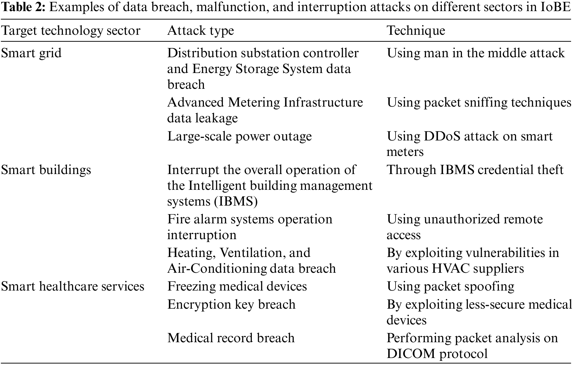
A comprehensive analysis of possible vulnerabilities in smart factories, smart grids, digital healthcare, smart buildings, and intelligent transport systems was provided in [6], assessing potential attack surfaces and security threats. Advanced metering infrastructure, energy storage systems, energy management systems, and electric vehicle charging systems are potential attack surfaces in a smart grid [26–33]. Similarly, electronic medical equipment, medical information systems, and overall healthcare networking systems are potential attack surfaces in smart healthcare [34–37]. Furthermore, closed-circuit television systems, alarm systems, access control systems, heating, ventilation, and air conditioning, and integrated building management systems are possible attack surfaces in smart buildings and smart factories [38–44]. Furthermore, these attack surfaces are exposed to potential security threats, such as data breaches, data tampering, malfunction and interruption, malicious code infection, and sometimes physical damage to equipment. Table 2 summarize some potential vulnerabilities in the IoBE with their respective attack surfaces and security threats, focusing on smart grids, smart buildings, and smart healthcare.

Following the complex interconnection between heterogeneous environments, the data generated by an active player in the IoBE are mostly consumed by the other participants. Such complex data propagation and consumption facilitate sophisticated cyber threats that leverage weak links in an environment where security solution is weak or absent. Moreover, owing to the novelty of these threats, it will be difficult for security technologies to detect and identify them, as the convergence is occurring before such security scenarios are sufficiently considered [24]. Therefore, devising a robust threat detection technology, with the aforementioned scenarios in mind, is the primary step toward mitigating blended threats in the IoBE. Once blended threats are successfully detected, the next step is characterizing them and tracing their origins by identifying the subtle relationship between the intrinsic nature of those threats.

Furthermore, machine learning models benefitted greatly from the ever-growing amount of massive data collected from various sources [45]. Consequently, when sufficiently designed and fine-tuned, these models have shown remarkable success in easily fitting to any given problem space [46,47]. Similarly, deep learning approaches, as discussed in Section 1, play an invaluable role in designing effective network intrusion detection systems. Therefore, we designed a robust approach for blended threat detection in the IoBE using an ensemble of heterogeneous probabilistic autoencoders. In doing so, we leveraged the corresponding advantages of Conv-VAE and LSTM-VAE to effectively model the dynamic characteristics of network traffic and determine the subtle relationship between the intrinsic nature of blended threats.

4  Proposed Solution

The proposed approach encompasses an ensemble of heterogeneous autoencoder-based models, Conv-VAE and LSTM-VAE, to model the spatial and temporal characteristics, respectively, of network traffic. Similarly, we used a probabilistic autoencoding approach to address the expected variability in the distribution of IoBE data. In standard autoencoders, the reconstruction error, which is an essential parameter for characterizing the network traffic, is computed based only on the difference between the reconstruction and the original input. This deterministic nature makes it difficult to calculate the representative reconstruction error if the underlying input variables are heterogeneous (as in IoBE data). However, probabilistic autoencoders address this problem by calculating the probabilistic reconstruction error based on both the reconstruction error and the variance parameter of the respective distribution of each unit of heterogeneous input data. Furthermore, to address the possible large false alarm rate due to heterogeneity in the IoBE data, we devised an optimal threshold computation module that determines the best representative threshold value based on the results of both models. A further explanation of this module is provided in Section 4.3. Fig. 4 illustrates the overall design of the proposed solution.

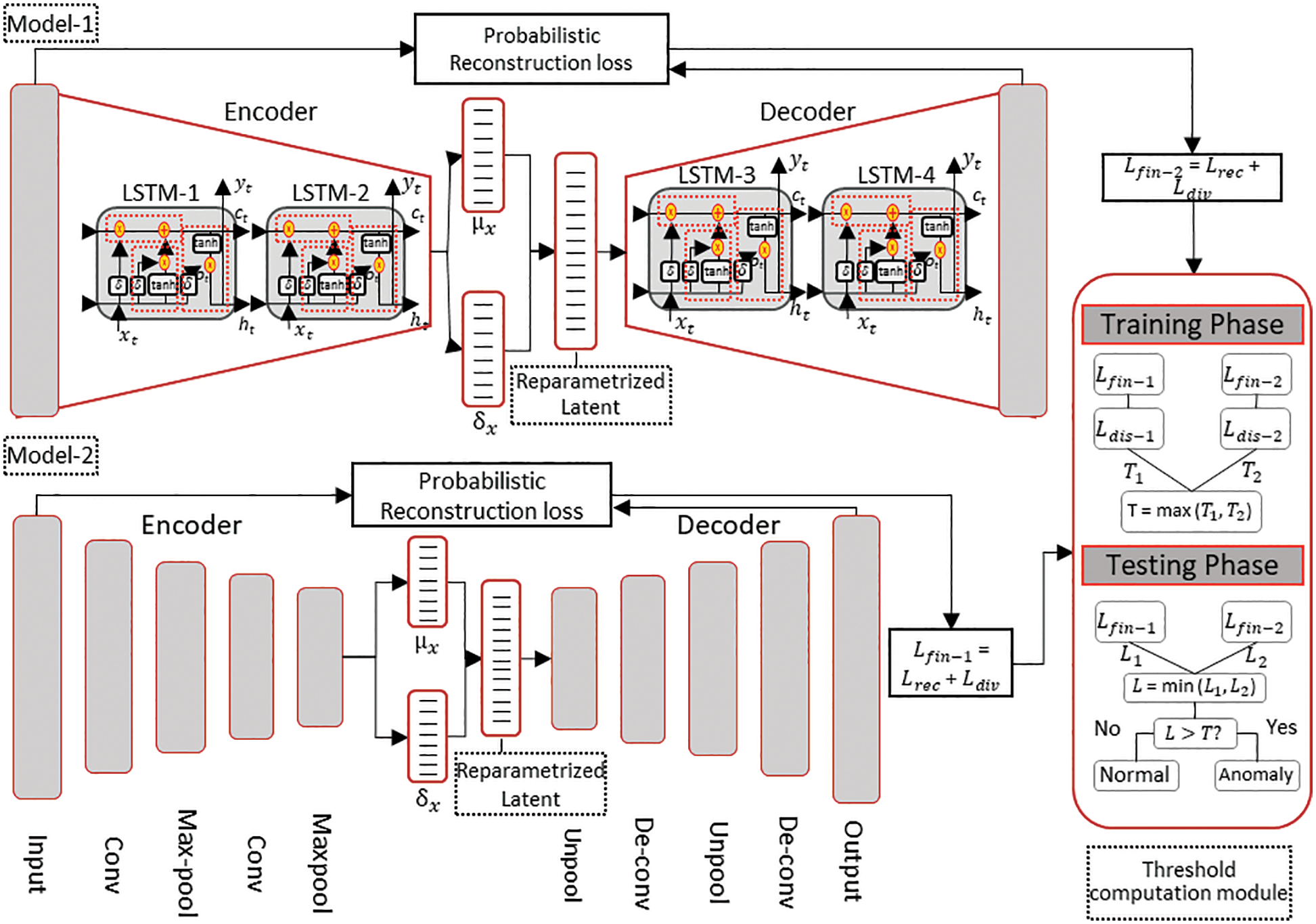
Figure 4: Overall design of the proposed solution

4.1 Convolution Variational Autoencoder (Conv-VAE) Modeling

For a sequence S={s1, s1s2s3…sn} of network traffic, where si is a feature of the traffic and Ns is the total number of data points in the dataset, the dimensionality of the dataset is x∈Rsi×Ns. Given an input dataset x characterized by an unknown probability distribution p(x), the objective of training the Conv-VAE is to model or approximate the true distribution p of the data using a parametrized distribution pθ, as shown in Eq. (8). However, because of the computational complexity of calculating pθ(x), the VAE uses an extra function qϕ(z|x) to approximate the posterior distribution by calculating a distribution z given input x. As a result, qθ(z|x)≈pθ(z|x), where ϕ, is a set of real values that parametrizes q.

pϕ(x)=∫pθ(x˙|z)pθ(z)dz(8)

where p(x) is the probability of the input data x, pθ(x) is a parametrized probability of input data x,pθ(z) is a parametrized probability of latent space z, pθ(x˙|z) is a parametrized probability of reconstructed data x˙ given latent space z, and qϕ(z|x) is an approximated posterior of latent space z given input data x.

Therefore, training the Conv-VAE entails finding a good probabilistic autoencoder by crafting the encoder part to calculate the conditional likelihood distribution qϕ(z|x), and designing the decoder part to approximate the posterior distribution pθ(x˙|z), as shown in Fig. 5. This way, the parameters θ and ϕ will be co-optimized to reduce the probabilistic reconstruction error between the input and generated data, and qϕ(z|x) will be as close as possible to pθ(z|x). The mean squared error is used to compute the reconstruction loss, whereas the KL divergence, DKL(pθ(x˙|z)||pθ(z)), is used to compute the difference between the probability distributions of q and p over the same variable x by squeezing qϕ(z|x) under pθ(z|x). (Algorithm 1) is used to implement the aforementioned training process of the Conv-VAE network.

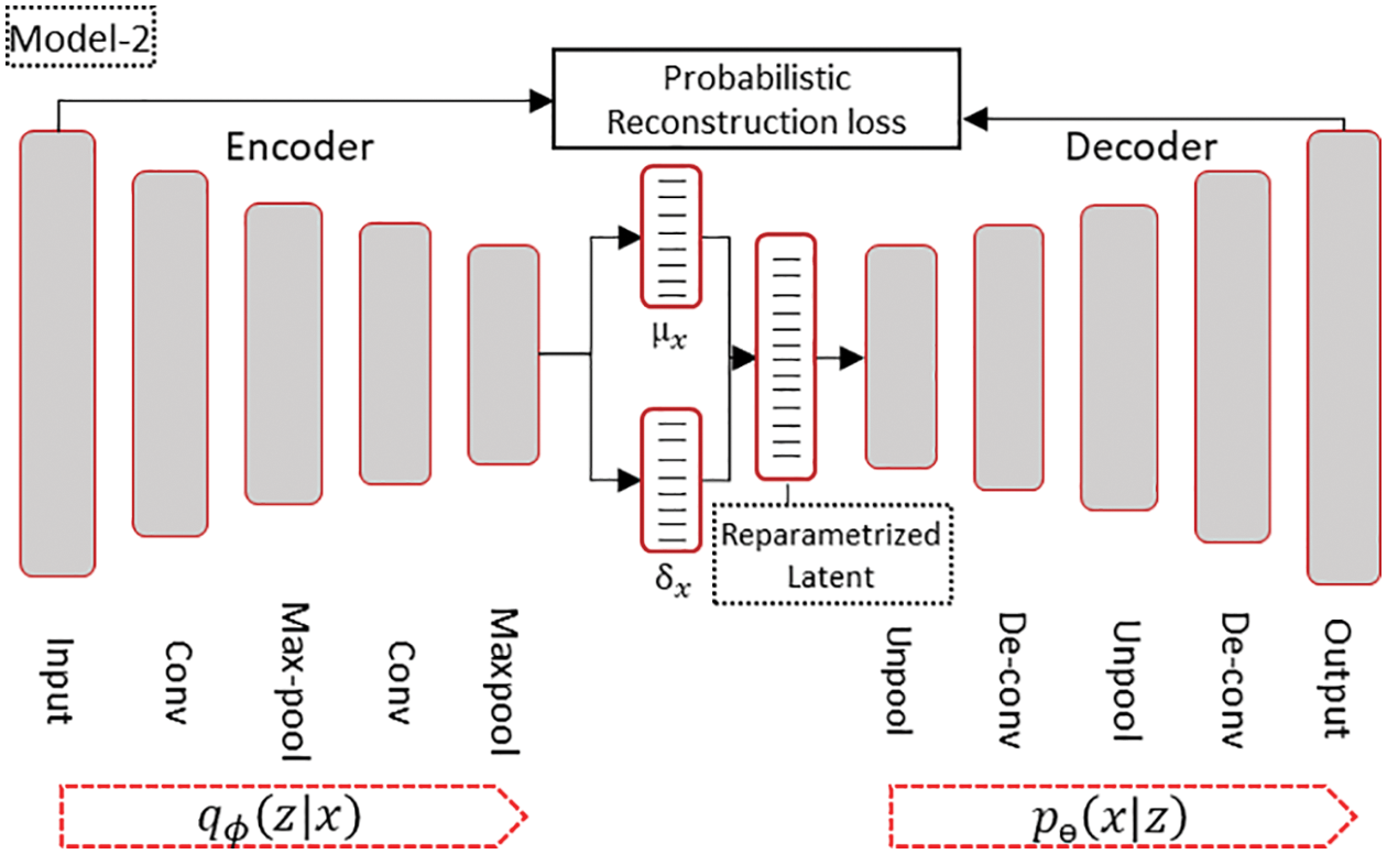
Figure 5: Implemented Conv-VAE model structure

We used one-dimensional, two stages of convolution and max pooling from the encoder side and the reciprocal structure—unpooling and deconvolution layers—in the decoder part, when modeling the Conv-VAE, as shown in Fig. 5. A kernel size of 4 with a feature space depth ranging from 8 to 32 channels for the encoder and the reverse was used for the decoder part. The stride and padding sizes were determined through trial and error to conform to the dimensionality requirements of the intermediate layers without compromising performance. We also added dropout with a probability of 0.3 per hidden layer to address the overfitting problem and trained the network for 100 epochs using the Adam optimizer with a learning rate of 1e−4.

4.2 LSTM Variational Autoencoder (LSTM-VAE) Modeling

The LSTM-VAE is modeled in the same way and with the same objective as the Conv-VAE, reducing the probabilistic reconstruction error between the input and generated data and bringing the distribution of qϕ(z|x) as close as possible to pθ(z|x), using the mean squared error and KL divergence loss, respectively, as shown in Fig. 6. (Algorithm 2) is used to train two LSTM cells in each encoder and decoder part. The training process is same as of the algorithm 1 with slight difference in the trainable parameters (line 3 and 7–10). Similarly, we added dropout with a probability of 0.3 after each hidden layer to address the overfitting problem. Finally, we trained the network for 100 epochs using the Adam optimizer with a learning rate of 1e−5.

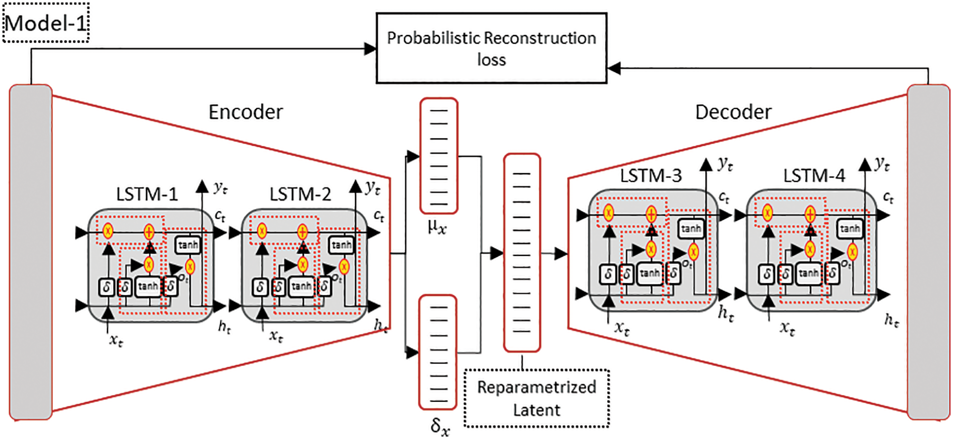
Figure 6: Implemented LSTM-VAE model structure

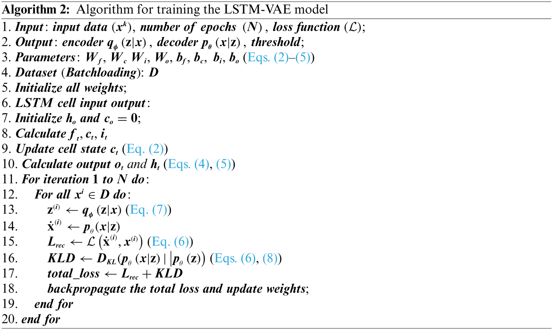
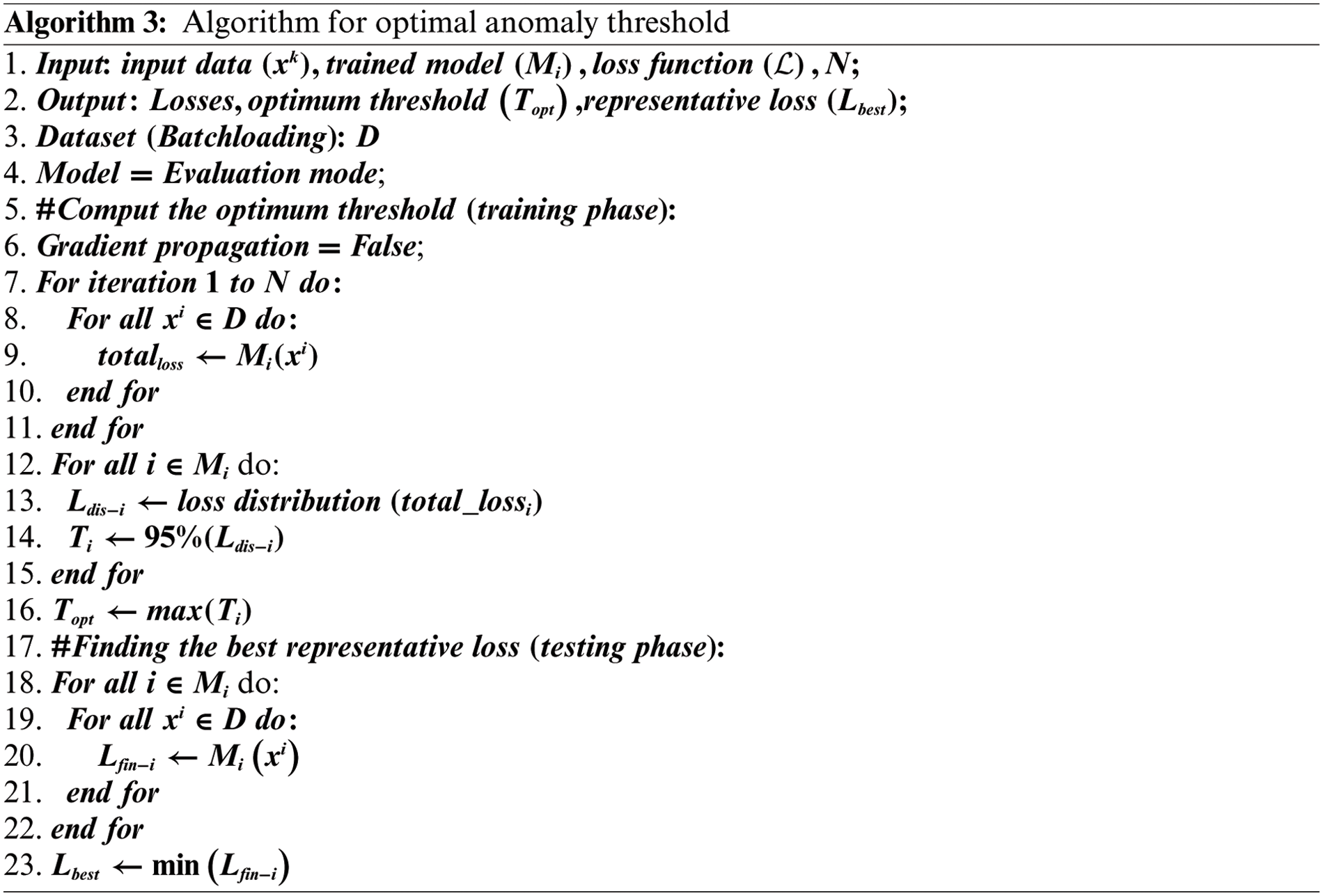
4.3 Computing Anomaly Threshold

In a classical approach, anomaly detection is performed by finding the best representative corresponding conditional likelihood distribution qϕ(z|x) for the normal data points and categorizing any input that does not follow the distribution as anomalous. The probabilistic reconstruction loss of any unseen data point will be larger than that of a benign data point. Therefore, the model can easily recognize anomalous data points as outliers by setting a threshold for the reconstruction loss. However, such an approach will suffer from a high rate of false alarms and performance degradation if insufficiently modeled. Furthermore, the convergence of various heterogeneous environments in the IoBE makes things worse, as it is likely that the underlying detection models will experience numerous unmodeled behaviors. To address this problem, we devised an optimal threshold computation module that generalizes and computes the anomaly threshold to effectively discriminate between anomalous and benign traffic. This was performed using an ensemble of total probabilistic losses from both Conv-VAE and LSTM-VAE, as shown in Fig. 7.

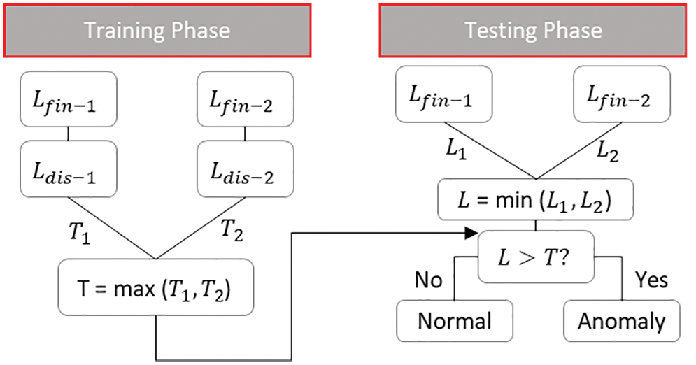
Figure 7: Proposed optimal threshold computation model

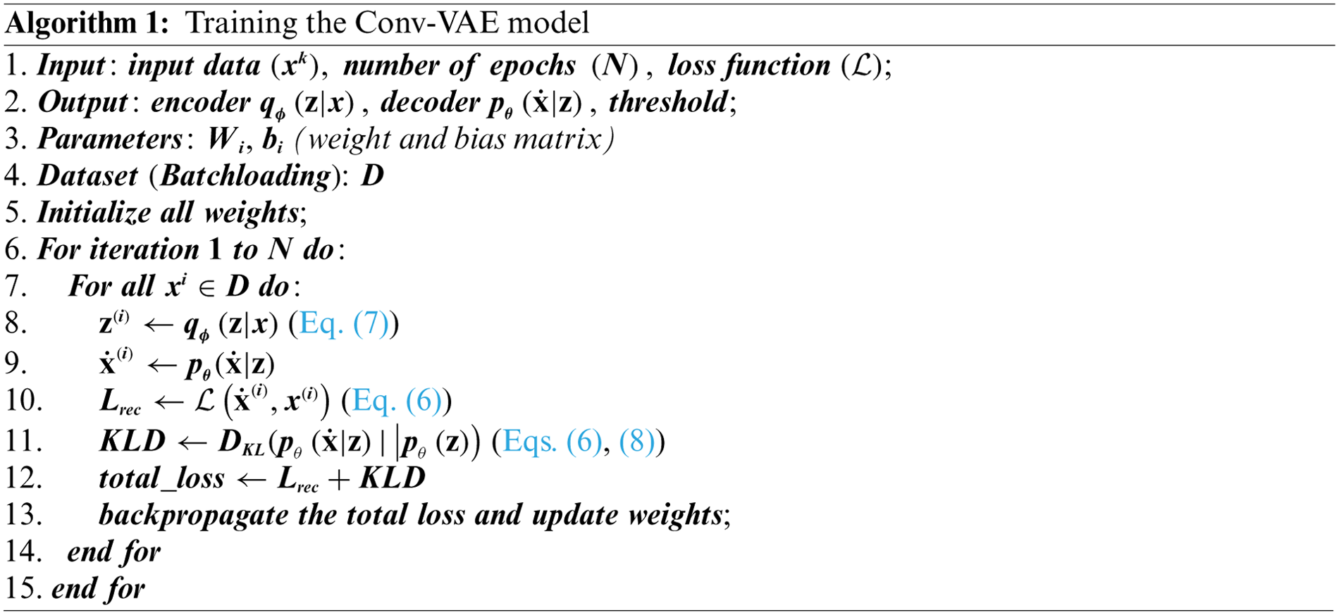
(Algorithm 3) is used to compute the anomaly threshold in the training phase and to determine the representative probabilistic total loss for each data point in the testing phase. In the training phase, the anomaly threshold for each model (T1,T2) is computed based on their respective loss distributions Ldis−1,Ldis−2, (Algorithm 3, line 3). We used the Z-score with two-sigma (95%) to set a threshold (T1,T2), and the maximum of these values, max(T1,T2), is set to be the optimum threshold T (Algorithm 3, line 14–16). In the testing phase, a minimum of the corresponding probabilistic final loss from each model, min(L1,L2), is computed and compared with the optimum threshold, T, to identify anomalies (Algorithm 3, line 18–20). L1 and L2 are the corresponding final losses computed by both probabilistic autoencoders, that is, Lfin−1 and Lfin−2, respectively. The best representative loss for each data point is compared with the optimum threshold for the anomaly decision in the training phase (Algorithm 3, line 23).

5  Implementation

5.1 Experimental Setting

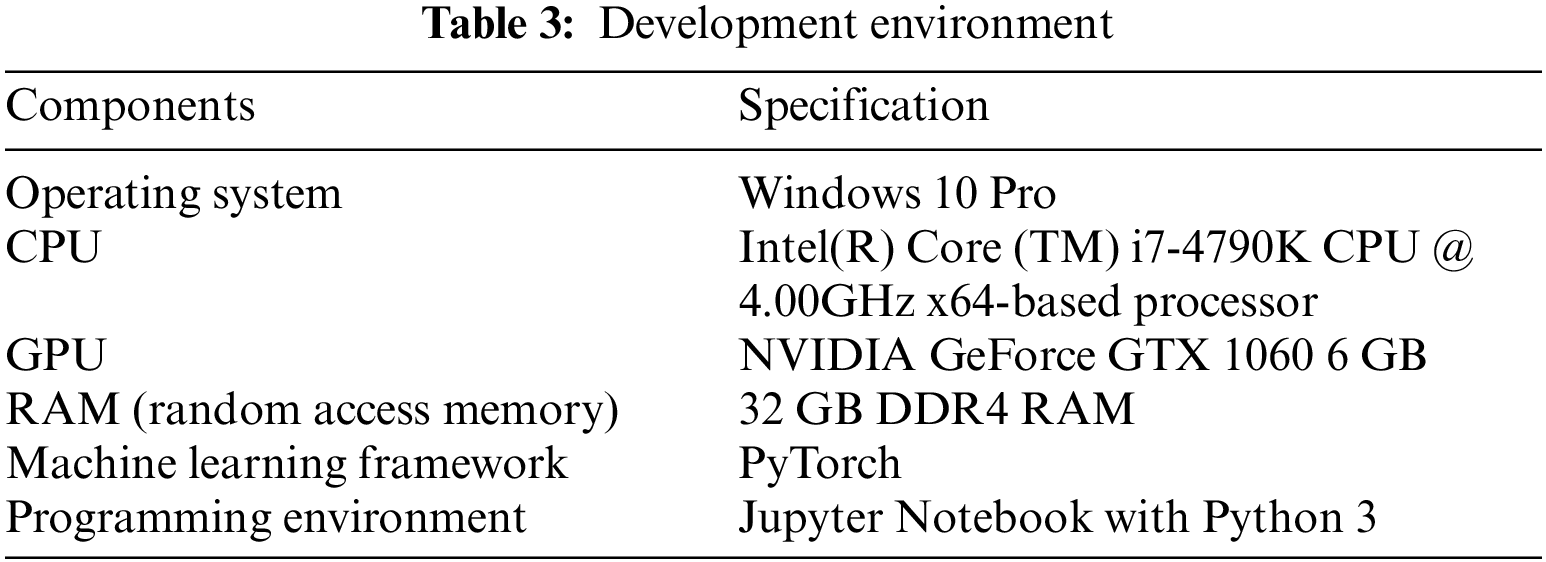
The model was implemented in the Python programming language using the PyTorch framework and Jupyter Notebook. Table 3 shows our development environment. The implementation environment and experimental setup explained in this section also works for other network intrusion detection datasets such as NSL-KDD.

The model was trained using the Adam optimizer along with other fine-tuned hyperparameters such as training epochs, batch size, learning rate, and loss. The mean square error (MSE) was used to measure the probabilistic reconstruction error, as the latent space vector of our models follows a Gaussian distribution. A binary cross entropy (BCE) loss would have performed better in a latent space vector with a multinomial distribution (such as classification tasks). We used a mini-batch training approach in which the optimizer updated the weight matrix for each input data, but the gradient was reset for each mini-batch computation. We used the probabilistic reconstruction error and KL divergence loss to evaluate the model using the validation data for each epoch during the training phase. Fig. 8 illustrates the overall training process of the proposed solution (excluding the optimum anomaly threshold computation process). Furthermore, the dataset was split into training, validation, and test groups for evaluation. We first split the dataset into 80% training and 20% testing sets, and then separated only the normal traffic from the training set for model training. Finally, the model’s performance was evaluated by measuring the accuracy, precision, recall, and F1-score from the results of a single run on the test dataset. Further elaboration on the evaluation matrices is provided in Section 4.3.

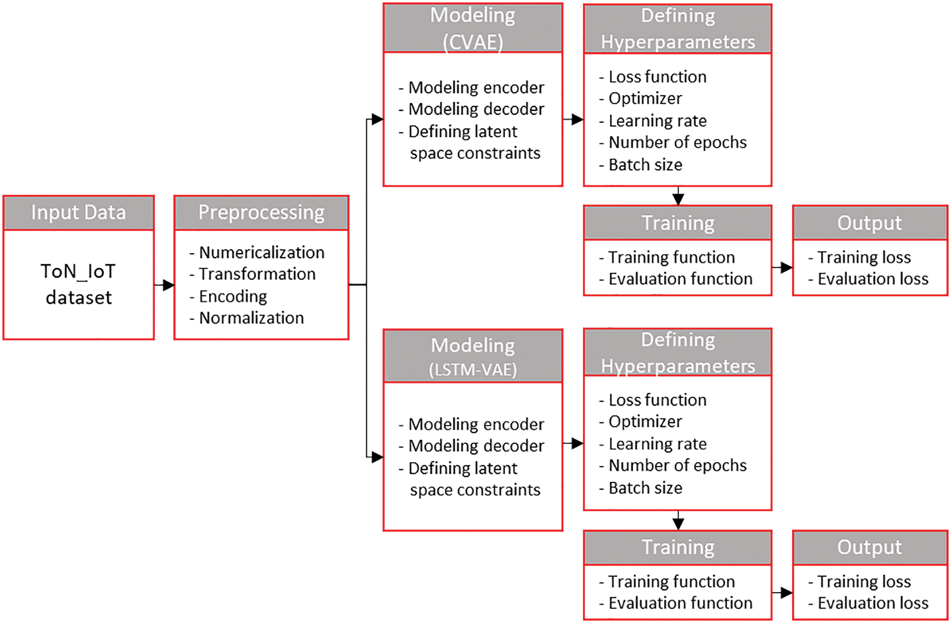
Figure 8: Overall training process of the proposed solution (excluding the optimal threshold computation process)

5.2 Dataset

As explained in Section 2.3, the IoBE is a blended environment in which various technology sectors converge to form an indivisible whole. To prepare a proof-of-concept for our proposed work, we needed a dataset that was created considering such a converged environment. However, obtaining a comprehensive dataset was challenging. Therefore, we chose to use the ToN_IoT dataset, which is closer to our requirements, as it was collected under conditions that partially resemble those of the IoBE. The dataset was collected from heterogeneous data sources including IoT and Industrial IoT (IIoT) sensors telemetry data, network traffic, and operating system logs, (Windows 7, Windows 10, Ubuntu 14 TLS and 18 TLS) [48,49]. A new testbed including IoT and IIoT networks was created to resemble the realistic heterogeneity of medium scale Industry 4.0, based on the interaction between network elements and IoT/IIoT systems with the three layers of Edge, Fog, and Cloud [50]. Furthermore, the dataset encompasses numerous normal and cyber-attack events against web applications, IoT gateways, and computer systems collected from network traffic, Windows audit traces, Linux audit traces, and telemetry data of IoT services. The Train_Test_Network dataset was used to train and evaluate the proposed model [51]. The distribution and other statistical information of the dataset are discussed in Section 5.3 along with discussing the preprocessing operation.

5.3 Preprocessing

Preprocessing encompasses numericalization, encoding, and normalization. The numericalization and encoding steps are used to convert all non-numerical (categorical) features into numbers and later to binary features using a one-hot encoding technique. Similarly, the normalization step is used to mitigate the impact of scale variation across different features in the dataset; thus, features with large values do not influence the outcome. This step is performed using a standard scaler. The Train_Test_Network_dataset contains 461,043 records, of which 300,000 are labeled as “normal” and 161,043 are labeled as “anomalous” Table 4. Furthermore, the anomalous category includes attacks such as backdoors, DDoS, DoS, injection, ransomware, and scanning, including numerical and categorical features. Fig. 9 illustrates the distribution of attack types in the Train_Test_Network_dataset.

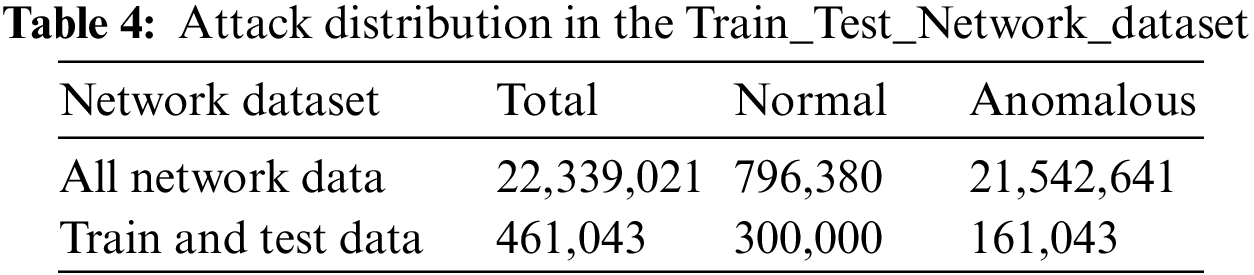
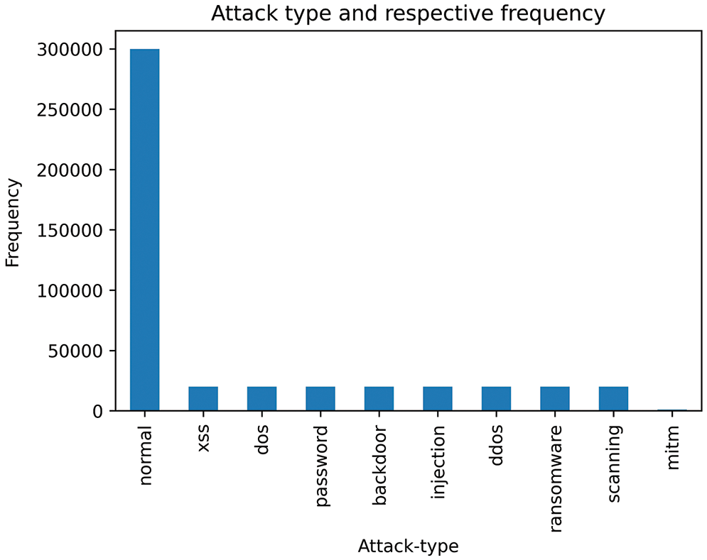
Figure 9: Histogram of attack data points in TON_IoT dataset

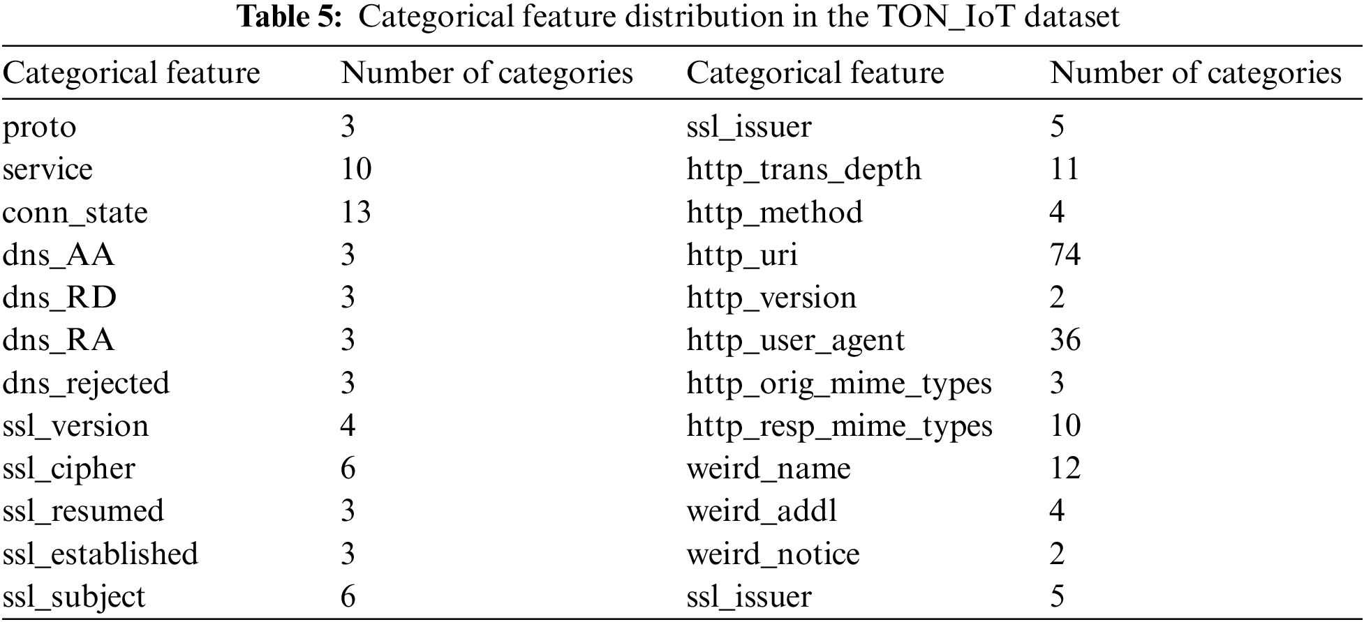
The one-hot encoding process takes a matrix of integers, denoting the values taken by categorical features, and converts them into n-dimensional vectors of binary code, where the value of “n” is determined by the total number of attributes in the categorical feature. It is assumed that the input features take values within the range (0, n). Therefore, we first encode the features into labels and then transform every category into a number. For example, the single feature “http_version” is encoded into two features using one-hot encoding. As shown in Table 5, there are 24 categorical features in the dataset; the maximum number of distinct attributes per feature is 74, and the minimum is 2. Therefore, after applying one-hot encoding, the total number of features becomes 252, of which 233 are categorical features and the rest are numeric features.

The normalization step is performed using a standard scaler, which scales the data to unit variance by making the mean equal to zero following the standard normal distribution. This type of normalization technique is useful for features that follow a normal distribution. Each point x of the input data was converted to the equivalent point in a standard normal distribution z, using Eqs. (9) and (10).

z=x−μδ(9)

δ=∑(xi−μ)2N(10)

where δ,N,xi, and μ denote the standard deviation, feature size, data point, and mean of the intended features, respectively.

5.4 Evaluation Matrix

An experiment was conducted to investigate the performance of the proposed work in two ways: (1) by conducting an experiment on a dataset collected from an environment that closely resembles the IoBE (the ToN_IoT dataset), and (2) by evaluating its performance against a single autoencoder-based network intrusion detection methods. Performance metrics including accuracy, precision, recall, and F1-score were used to evaluate the overall performance of the proposed approach. The formulae used to calculate each performance matrix are given in Eqs. (11)–(14), respectively.

Accuracy=TP+TNTP+FP+FN+TN(11)

Precision=TPTP+FP(12)

Recall=TPTP+FN(13)

F1Score=2∗(Recall∗Precision)Recall+Precision(14)

In this context, true positive (TP) is the number of correctly labeled anomalous traffic samples, true negative (TN) is the number of correctly labeled normal traffic samples, false positive (FP) is the number of incorrectly labeled anomalous traffic samples, and false negative (FN) is the number of incorrectly labeled normal traffic samples.

6  Results and Discussion

6.1 Model Training Performance

In the training phase, inefficient model parameter definitions such as hyperparameter tuning, including learning rate, dropout probability, number of layers, and optimizer type, significantly affect the model performance. Over tuning results in overfitting to the training set, whereas under tuning results in poor performance. The training phase can be formulated as a multi-objective optimization problem where the objectives are to determine the optimal solution for the aforementioned model parameters. However, because this problem has no distinct solution, most researchers use an iterative searching approach, such as grid searching, to select the best candidates among a predefined set of values. The dropout probability randomly sets the portion of disconnecting neurons whenever applied, whereas the learning rate defines the optimal rate at which the model should minimize the difference between the ground truth and the expected outcome. The Adam optimizer is a popular and almost parameter-free optimization function that allows the learning rate to adapt over time. However, the initial learning rate must be set to avoid divergence.

After conducting rigorous experiments, we found two different sets of the best model parameters for both Conv-VAE and LSTM-VAE. The differences between the sets are probably due to the underlying variabilities in the model structure. The optimal dropout probability, number of layers, and learning rate for the Conv-VAE model were found to be 0.5, 3 per encoder-decoder, and 1e−4, respectively. The corresponding values for the LSTM-VAE were found to be 0.3, 3 per encoder-decoder, and 1e−5, respectively. Consequently, both models appeared to follow a satisfying trajectory in both the training and validation phases, as illustrated in Fig. 10. In both cases, the validation loss almost followed the trajectory of the training loss curve, which implies high precision of the hyperparameter tuning process, as shown in Figs. 10b and 10c.

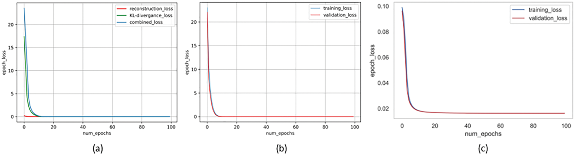
Figure 10: Loss vs. number of epochs: (a) training loss of Conv-VAE vs. number of epochs; (b) training and validation loss of Conv-VAE vs. number of epochs; (c) training and validation loss of LSTM_VAE vs. number of epochs

Initially, we set an equal learning rate for both models, and the process continued to perform well until we re-evaluated the models by increasing the number of training epochs (from 100 to 300). In this case, the LSTM-VAE model frequently experienced a sudden divergence after a long convergence duration, whereas the Conv-VAE model continued to perform well. The problem was resolved by setting the dropout probability to 0.5 and minimizing the learning rate by a factor of 10 for the LSTM-VAE. Despite the longer training duration, the small learning rate helped the LSTM-VAE model to learn a better set of weights for the given input data space, as shown in Fig. 10c. However, the Conv-VAE smoothly converged, starting from a significantly larger loss, as shown in Figs. 10a and 10b.

6.2 Optimal Threshold Computation

Despite the underlying heterogeneity, both models converged to approximately similar loss values from different starting points. Similarly, both models exhibited interesting characteristics for modeling the distribution of the input data space. These two points motivated us to use an ensemble of both heterogeneous models to address the dynamic behavior of the IoBE. The corresponding histogram of model loss on benign test data points indicates that both models follow a normal distribution, as shown in Figs. 11a and 12a. Therefore, we set the anomaly threshold value for both models by using the Z-score rule with two-sigma (95%). Fig. 11a illustrates the test loss distribution of normal data points for Conv-VAE, whereas Fig. 12a illustrates the corresponding results for LSTM-VAE.

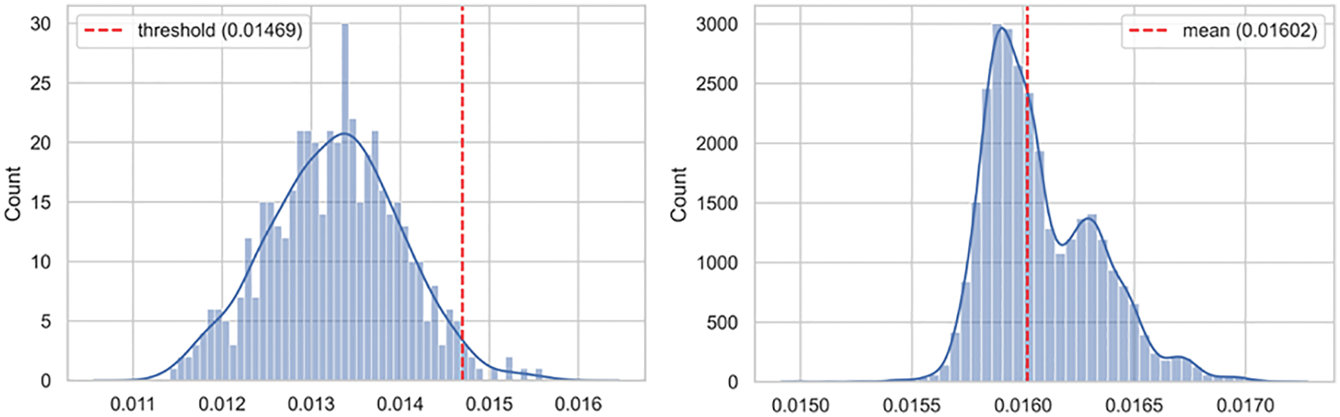
Figure 11: Loss distribution of Conv-VAE: (a) benign test dataset; (b) anomalous test dataset

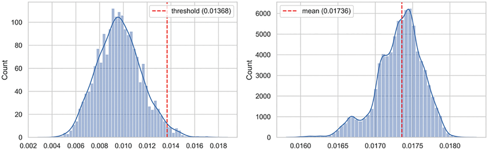
Figure 12: Loss distribution of LSTM-VAE: (a) benign test dataset; (b) anomalous test dataset

In contrast, the corresponding histogram of the model loss for the test data containing only attack data points shows that both models follow different distributions, as shown in Figs. 11b and 12b. The Conv-VAE model appears to follow a multimodal log-normal distribution, whereas the LSTM-VAE appears to follow a flipped multimodal log-normal distribution. As illustrated in Figs. 11 and 12, both models performed well in separating the corresponding distribution of benign (test) and attack (test) data points with minimal overlapping. The greater the overlap, the poorer the model performance. The exhibited multimodality indicates that both networks perform well in modeling different attack types. However, the most important point is that both models exhibited almost the exact mirror of the distribution, log-normal, and flipped log-normal. This is an interesting point, as it indicates that both networks are clearly specialized in the process of modeling different attacks. Identifying the exact sets of attacks for which the models are more specialized requires further experimental analysis with sufficient model explanation, particularly using explainable artificial intelligence (XAI) frameworks. However, from a general point of view, we observe that combining both networks will help detect various types of attacks, which is the fundamental requirement for effective blended threat detection in the IoBE.

We tested the classification performance of the proposed solution by changing the problem space to a supervised problem. This was performed by making the model predict a correct label for the underlying test dataset. The proposed ensemble threshold computation module calculated the optimal threshold for the anomaly decision and the corresponding best representative total loss for each test data point. The anomaly classification was then performed by comparing these two values. In this way, we evaluated the model performance based on the classification recall, F1-score, accuracy, and precision results, as shown in Table 6. Furthermore, we evaluated the model performance based on the receiver operating characteristic (ROC) curve. The proposed solution demonstrated remarkable performance by producing a larger area under the curve (AUC), as shown in Fig. 13. The ROC-AUC curve was generated using the true label of the test set and the corresponding best representative loss for each data point. A larger AUC indicates better model performance in minimizing the false positive rate. Moreover, we conducted a performance comparison with various single autoencoder-based network intrusion detection approaches: autoencoder, variational autoencoder, convolutional variational autoencoder, and long short-term memory autoencoder. The results indicated that the proposed model outperformed all the models, demonstrating F1-scores 3.99%, 1.95%, 1.92%, and 2.69% greater than those of the respective models, as shown in Table 6.

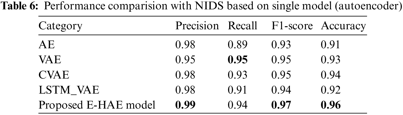
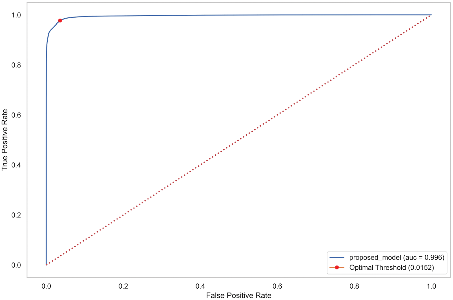
Figure 13: ROC curve of the proposed approach

7  Conclusions

As previously described, blended threats can explore various attack surfaces in the IoBE, in which many technology sectors converge, exploiting the respective security vulnerabilities in the environment. Furthermore, such attacks exhibit strong intrinsic mutual effects with each other. A threat detection and identification system developed by considering such an environment is the primary step that must be taken to mitigate blended threats. Therefore, in this paper, we presented an intrusion detection system for the IoBE, using an ensemble of heterogeneous autoencoders to mitigate the possible impact and dimensionality of the new attack surfaces resulting from the convergence of different technology sectors. An extensive experiment was conducted on ToN-IoT network intrusion detection datasets, in which the proposed solution achieved 96.02% detection accuracy. Furthermore, we conducted a performance comparison against various single model (autoencoder)-based network intrusion detection approaches: autoencoder, variational autoencoder, convolutional variational autoencoder, and long short-term memory variational autoencoder. The proposed model outperformed all compared models, demonstrating F1-score improvements of 4.99%, 2.25%, 1.92%, and 3.69%, respectively. In the future, we plan to further enhance the proposed solution by exploiting the model decision space using XAI frameworks. Furthermore, we plan to extend the proposed solution to blended threat identification and response.

Funding Statement: This work was supported by the National Research Foundation of Korea (NRF) grant funded by the Korean government (MSIT) (No. 2021R1A2C2011391) and was supported by the Institute of Information & communications Technology Planning & Evaluation (IITP) grant funded by the Korea government (MSIT) (No. 2021-0-01806, Development of security by design and security management technology in smart factory).

Conflicts of Interest: The authors declare that they have no conflicts of interest to report regarding the present study.

References

1. X. Fang, S. Misra, G. Xue and D. Yang, “Smart grid—the new and improved power grid: A survey,” IEEE Communications Surveys & Tutorials, vol. 14, no. 4, pp. 944–980, 2011. [Google Scholar]
2. R. Apanaviciene, A. Vanagas and P. A. Fokaides, “Smart building integration into a smart city (SBISCDevelopment of a new evaluation framework,” Energies, vol. 13, no. 9, pp. 2190, 2020. [Google Scholar]
3. R. Agrawal and S. Prabakaran, “Big data in digital healthcare: Lessons learnt and recommendations for general practice,” Heredity, vol. 124, no. 4, pp. 525–534, 2020. [Google Scholar] [PubMed]
4. M. Farmanbar, K. Parham, Ø. Arild and C. Rong, “A widespread review of smart grids towards smart cities,” Energies, vol. 12, no. 23, pp. 4484, 2019. [Google Scholar]
5. B. Morvaj, L. Lugaric and S. Krajcar, “Demonstrating smart buildings and smart grid features in a smart energy city,” in Proc. 3rd Int. Youth Conf. on Energetics (IYCE), Leiria, Portugal, pp. 1–8, 2011. [Google Scholar]
6. M. Lee, J. Jang-Jaccard and J. Kwak, “Novel architecture of security orchestration, automation and response in internet of blended environment,” Computers, Materials & Continua, vol. 73, no. 1, pp. 199–223, 2022. [Google Scholar]
7. J. Cowie, A. Ogielski, B. J. Premore and Y. Yuan, “Global routing instabilities triggered by Code Red II and Nimda worm attacks,” Renesys Corporation, vol. 77, no. 1, pp. 1–11, 2001. [Google Scholar]
8. A. Machie, J. Roculan, R. Russell and M. V. Velzen, Nimda worm analysis. San Mateo, CA, USA: SecurityFocus, 2001. [Online]. Available at: http://www.di-srv.unisa.it/professori/ads/corso-security/www/CORSO-0102/NIMDA/link_locali/010921-Analysis-Nimda-v2.pdf [Google Scholar]
9. T. M. Chen and J. M. Robert, “The evolution of viruses and worms,” in Statistical Methods in Computer Security. Boca Raton, Florida, USA: Chemical Rubber Company (CRC) Press, pp. 289–310, 2004. [Google Scholar]
10. B. Zhang, Y. Yu and J. Li, “Network intrusion detection based on stacked sparse autoencoder and binary tree ensemble method,” in Proc. IEEE Int. Conf. on Communications (ICC) Workshops, Kansas City, MO, USA, pp. 1–6, 2018. [Google Scholar]
11. B. Yan and G. Han, “Effective feature extraction via stacked sparse autoencoder to improve intrusion detection system,” IEEE Access, vol. 6, pp. 41238–41248, 2018. [Google Scholar]
12. M. Al-Qatf, Y. Lasheng, M. Al-Habib and K. Al-Sabahi, “Deep learning approach combining sparse autoencoder with SVM for network intrusion detection,” IEEE Access, vol. 6, pp. 52843–52856, 2018. [Google Scholar]
13. H. Liu and B. Lang, “Machine learning and deep learning methods for intrusion detection systems: A survey,” Applied Sciences, vol. 9, no. 20, pp. 4396, 2019. [Google Scholar]
14. Z. Wu, X. Wang, Y. G. Jiang, H. Ye and X. Xue, “Modeling spatial-temporal clues in a hybrid deep learning framework for video classification,” in Proc. 23rd ACM Int. Conf. on Multimedia, Brisbane, Australia, pp. 461–470, 2015. [Google Scholar]
15. J. Wang, Y. Yang, J. Mao, Z. Huang, C. Huang et al., “Cnn-rnn: a unified framework for multi-label image classification,” in Proc. IEEE Conf. on Computer Vision and Pattern Recognition (CVPR), Las Vegas, NV, USA, pp. 2285–2294, 2016. [Google Scholar]
16. C. Chen, K. Li, S. G. Teo, X. Zou, K. Li et al., “Citywide traffic flow prediction based on multiple gated spatio-temporal convolutional neural networks,” ACM Transactions on Knowledge Discovery from Data, vol. 14, no. 4, pp. 1–23, 2020. [Google Scholar]
17. M. Sundermeyer, I. Oparin, J. L. Gauvain, B. Freiberg, R. Schlüter et al., “Comparison of feedforward and recurrent neural network language models,” in Proc. IEEE Int. Conf. on Acoustics, Speech and Signal Processing, Vancouver, BC, Canada, pp. 8430–8434, 2013. [Google Scholar]
18. Z. C. Lipton, J. Berkowitz and C. Elkan, “A critical review of recurrent neural networks for sequence learning,” arXiv preprint arXiv:1506.00019, 2015. [Google Scholar]
19. A. Sherstinsky, “Fundamentals of recurrent neural network (RNN) and long short-term memory (LSTM) network,” Physica D: Nonlinear Phenomena, vol. 404, no. 8, pp. 132306, 2020. [Google Scholar]
20. Y. Yu, X. Si, C. Hu and J. Zhang, “A review of recurrent neural networks: LSTM cells and network architectures,” Neural Computation, vol. 31, no. 7, pp. 1235–1270, 2019. [Google Scholar] [PubMed]
21. J. Zhai, S. Zhang, J. Chen and Q. He, “Autoencoder and its various variants,” in Proc. IEEE Int. Conf. on Systems, Man, and Cybernetics (SMC), Miyazaki, Japan, pp. 415–419, 2018. [Google Scholar]
22. Y. Wang, H. Yao and S. Zhao, “Auto-encoder based dimensionality reduction,” Neurocomputing, vol. 184, no. 4, pp. 232–242, 2016. [Google Scholar]
23. D. P. Kingma and M. Welling, “An introduction to variational autoencoders,” Foundations and Trends® in Machine Learning, vol. 12, no. 4, pp. 307–392, 2019. [Google Scholar]
24. K. Zhang, J. Ni, K. Yang, X. Liang, J. Ren et al., “Security and privacy in smart city applications: Challenges and solutions,” IEEE Communications Magazine, vol. 55, no. 1, pp. 122–129, 2017. [Google Scholar]
25. H. Hejazi, H. Rajab, T. Cinkler and L. Lengyel, “Survey of platforms for massive IoT,” in Proc. IEEE Int. Conf. on Future IoT Technologies (future IoT), Eger, Hungary, pp. 1–8, 2018. [Google Scholar]
26. D. Grochocki, J. H. Huh, R. Berthier, R. Bobba, W. H. Sanders et al., “AMI threats, intrusion detection requirements and deployment recommendations,” in Proc. 3rd IEEE Int. Conf. on Smart Grid Communications (SmartGridComm), Tainan, Taiwan, pp. 395–400, 2012. [Google Scholar]
27. A. Anwar, A. N. Mahmood and Z. Tari, “Identification of vulnerable node clusters against false data injection attack in an AMI based smart grid,” Information Systems, vol. 53, no. 1, pp. 201–212, 2015. [Google Scholar]
28. Y. Guo, C. Ten, S. Hu and W. W. Weaver, “Preventive maintenance for advanced metering infrastructure against malware propagation,” IEEE Transactions on Smart Grid, vol. 7, no. 3, pp. 1314–1328, 2015. [Google Scholar]
29. N. Kharlamova, S. Hashemi and C. Træholt, “Data-driven approaches for cyber defense of battery energy storage systems,” Energy and Artificial Intelligence, vol. 5, no. 4, pp. 100095–100103, 2021. [Google Scholar]
30. J. Sun, P. Li and C. Wang, “Optimise transient control against DoS attacks on ESS by input convex neural networks in a game, Sustainable Energy,” Grids and Networks, vol. 28, pp. 100535–100547, 2021. [Google Scholar]
31. T. Nasr, S. Torabi, E. B. Harb, C. Fachkha and C. Assi, “Power jacking your station: in-depth security analysis of electric vehicle charging station management system,” Computer & Security, vol. 112, no. 6, pp. 102511, 2022. [Google Scholar]
32. A. Tang, S. Sethumadhavan and S. Stolfo, “CLKSCREW: Exposing the perils of security-oblivious energy management,” in 26th USENIX Security Symp., Vancouver, BC, Canada, pp. 1057–1074, 2017. [Google Scholar]
33. P. Zhao, Z. Cao, D. D. Zeng, C. Gu, Z. Wang et al., “Cyber-resilient multi-energy management for complex systems,” IEEE Transactions on Industrial Informatics, vol. 18, no. 3, pp. 2144–2159, 2021. [Google Scholar]
34. M. Khera, “Think like a hacker: Insights on the latest attack vectors (and security controls) for medical device applications,” Journal of Diabetes Science and Technology, vol. 11, no. 2, pp. 207–212, 2017. [Google Scholar] [PubMed]
35. A. K. Pandey, A. I. Khan, Y. B. Abushark, M. M. Alam, A. Agrawal et al., “Key issues in healthcare data integrity: Analysis and recommendations,” IEEE Access, vol. 8, pp. 40612–40628, 2020. [Google Scholar]
36. A. H. Seh, M. Zarour, M. Alenezi, A. K. Sarkar, A. Agrawal et al., “Healthcare data breaches: Insights and implications,” Healthcare, vol. 8, no. 2, pp. 133–151, 2020. [Google Scholar] [PubMed]
37. S. Oh, Y. Seo, E. Lee and Y. Kim, “A comprehensive survey on security and privacy for electronic health data,” International Journal of Environmental Research and Public Health, vol. 18, no. 18, pp. 9668, 2021. [Google Scholar] [PubMed]
38. S. Hong and S. Jeong, “The analysis of CCTV hacking and security countermeasure technologies: Survey,” Journal of Convergence for Information Technology, vol. 8, no. 6, pp. 129–134, 2018. [Google Scholar]
39. Y. Lee, N. Baik, C. Kim and C. Yang, “Study of detection method for spoofed IP against DDoS attacks,” Personal and Ubiquitous Computing, vol. 22, no. 1, pp. 35–44, 2018. [Google Scholar]
40. M. Shobana and S. Rathi, “IoT malware: An analysis of IoT device hijacking,” International Journal of Scientific Research in Computer Science, Engineering and Information Technology, vol. 3, no. 5, pp. 653–662, 2018. [Google Scholar]
41. V. Kharchenko, Y. Ponochovnyi, A. M. Q. Abdulmunem and A. Boyarchuk, “Security and availability models for smart building automation systems,” International Journal of Computing, vol. 16, no. 4, pp. 194–202, 2017. [Google Scholar]
42. M. Elnour, N. Meskin, K. Khan and R. Jain, “Application of data-driven attack detection framework for secure operation in smart buildings,” Sustainable Cities and Society, vol. 69, pp. 102816–102831, 2021. [Google Scholar]
43. H. Shin, J. Noh, D. Kim and Y. Kim, “The system that cried wolf: Sensor security analysis of wide-area smoke detectors for critical infrastructure,” ACM Transactions on Privacy and Security, vol. 23, no. 3, pp. 1–32, 2020. [Google Scholar]
44. R. Chan, F. Tan, U. Teo and B. Kow, “Vulnerability assessment of building management systems,” in Critical Infrastructure Protection XIV. Cham, Switzerland: Springer, pp. 209–220, 2020. [Online]. Available at: https://doi.org/10.1007/978-3-030-62840-6_10 [Google Scholar] [CrossRef]
45. L. Adeba Jilcha and J. Kwak, “Machine learning-based advertisement banner identification technique for effective piracy website detection process,” Computers, Materials & Continua, vol. 71, no. 2, pp. 2883–2899, 2022. [Google Scholar]
46. J. Wang, Y. Yang, T. Wang, R. Sherratt and J. Zhang, “Big data service architecture: A survey,” Journal of Internet Technology, vol. 21, no. 2, pp. 393–405, 2020. [Google Scholar]
47. T. Zhang and S. Bao, “A novel deep neural network model for computer network intrusion detection considering connection efficiency of network systems,” in 4th Int. Conf. on Smart Systems and Inventive Technology (ICSSIT), Tirunelveli, India, pp. 962–965, 2022. [Google Scholar]
48. A. Alsaedi, N. Moustafa, Z. Tari, A. Mahmood and A. Anwar, “TON_IoT telemetry dataset: a new generation dataset of IoT and IIoT for data-driven intrusion detection systems,” IEEE Access, vol. 8, pp. 165130–165150, 2020. [Google Scholar]
49. N. Moustafa, “New generations of internet of things datasets for cybersecurity applications based machine learning: TON_IoT datasets,” in Proc. eResearch Australasia Conf., Brisbane, Australia, pp. 21–25, 2019. [Google Scholar]
50. N. Moustafa, “A new distributed architecture for evaluating AI-based security systems at the edge: Network TON_IoT datasets,” Sustainable Cities and Society, vol. 72, pp. 102994–103008, 2021. [Google Scholar]
51. UNSW Canberra at the Australian Defence Force Academy, “The TON_IoT dataset,” 2021. [Accessed: 03-Jan-2022], 2022. [Online]. Available: https://cloudstor.aarnet.edu.au/plus/s/ds5zW91vdgjEj9i?path=%2FTrain_Test_datasets%2FTrain_Test_Network_dataset [Google Scholar]
Cite This Article
Copyright © 2023 The Author(s). Published by Tech Science Press.
This work is licensed under a Creative Commons Attribution 4.0 International License , which permits unrestricted use, distribution, and reproduction in any medium, provided the original work is properly cited.
Downloads
Citation Tools