An Optimized Chinese Filtering Model Using Value Scale Extended Text Vector

1  Introduction

With the popularity of Internet technology [1–4], consumers are increasingly motivated to comment online, which has made a large amount of comment data. Consumers usually make purchasing decisions on the comments because they cannot touch the real things online, being afraid that the description does not match the real thing [5–7]. However, with the rapid increase of online evaluations and the diversification of evaluations, it has become increasingly difficult for users to obtain helpful evaluations [8–12]. “Internet-paid posters” create hot spots, spread a lot of information, and make false comments by publishing many similar comments. They make a lot of meaningless and fake comments that seriously interfere with our access to real information, increasing the cost of time and the cost of trial. At the same time, their comments were highly biased [12–14], with a large number of comments in favor or against, aimed at “making the tempo” for some commercial purpose. There are two prominent features of their comments, one is repeated, and the other is emotion-orientated [15].

It is difficult to obtain valuable data from a large amount of comment data by only manual identification, so it has become an urgent problem to let the computer automatically screen valuable or worthless comments [16–18]. Therefore, filtering text content has important research value.

Text automatic classification [19] is based on a valuable classification model for training existing text collections. Then the trained model is applied to the unclassified dataset, making the classification accuracy of the model level as high as possible. Finally, similar text can be divided into the same category. This method is an efficient text categorization method, which is more accurate to implement categorical retrieval in massive data.

Specifically, the work of this article contains the following contents: The first is about data capture and calibration: 53,728 user comments of Wolf Warrior 2 are retrieved from the Douban movie, which is labeled based on value. The second is text feature extraction (also known as text vectorization). In this paper, the construction method of text synthesis vector is improved in the shallow neural network model according to the specific research content, which takes both text word frequency vector and text semantic vector into account. Experiments obtain the vectorization method with the highest accuracy with a combination of text word frequency vector, text semantic vector, and text value to construct a text filtering model. The third one is building a text-filtering model based on the BP neural network, a shallow neural network with the advantage of its simple structure and fast training speed.

The structure of this paper is as follows: in Chapter 2, we describe in detail what is the already done research regarding this particular problem; in Chapter 3, we introduce the overall process of this study; in Chapter 4, we analyze the experimental results; in Chapter 5, we summarized the full text and looked forward to the future work.

2  Related work

For Chinese text classification, the main research was divided into two aspects. One is the selection of a classification algorithm, and the other is the extraction of Chinese text features. Meanwhile, the false comments can be filtered out by calculating text similarity [20] and text sentimental tendencies [21] based on Chinese syntax and lexical structure.

The selection of classification algorithms is now mainly an improvement of machine learning algorithms, which have been proven to describe data better [22]. At present, the text classification algorithm based on machine learning can deal with most of the application scenarios, while it is an urgent problem to extract text features because of its great impact on classification accuracy.

In terms of feature extraction of Chinese text, Ma et al. [23]. Uses the LDA theme model to train the theme distribution of each news, obtaining the news recommendation list. Zhou et al. [24] introduce a variational inference algorithm for the Dirichlet process mixtures model (DPMM) for text clustering to disambiguate a person’s name. The extraction method of the text feature mentioned above mainly represents the text according to rules and combined features, which can only be applied to specific data sets because of a large amount of manpower in rulemaking and subjective comments.

The text should be converted into a form that the machine can recognize in the text categorization. Then the next categorization process can be effectively carried out. The common method is to vectorize the text. In recent years, the rise of deep learning has made the advantages of neural networks in text feature extraction more and more obvious, for example, the feature information of text at the semantic level can be mined. Google’s word2vec [25] for the first time demonstrated a way to convert words into vectors, which has been widely used in the field of natural language processing. Soon after the word2vec was proposed, the Google team proposed the doc2vec [26] method. When training the word vector, it also trained the documents vector, which is widely used in natural language processing.

In the text similarity calculation method, the distributed representation of sentences and documents [20,26] has a certain effect. Emotional analysis algorithms usually use natural language processing (NLP) [27], such as stem extraction, discourse tagging, etc. And emotional analysis algorithms use additional resources, such as dictionaries, or emotional dictionaries [28], to model the acquired documents. Document emotions are analyzed and detected by identifying distinctive features of the word frequency and discourse, inherent phrases, and negative and emphatic moods of the texts. Finally, emotional analysis algorithms follow the steps of emotion recognition [29] and then describe it as positive, negative, or neutral according to the document characteristics.

3  Proposed Methodology

The overall process of this study was as follows: First, sufficient data were obtained for the experiment. Next, the obtained data is calibrated and processed into a form that the computer can recognize called “Data vectorization”. Then, neural network model structures were established by setting hyperparameters, which could make the number of hidden layers and the number of neurons in each layer certain. Finally, complete neural network models were formed, and the model with the highest accuracy was screened out through testing. Fig. 1 is the flowchart of the process.

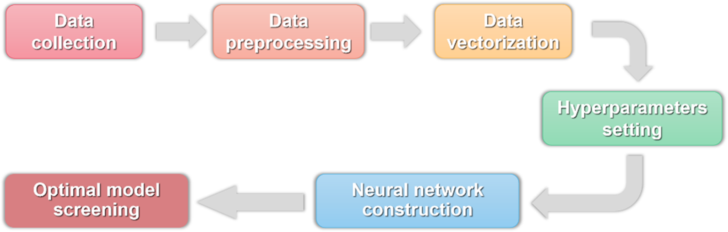
Figure 1: The flowchart of the research process

3.1 Data Collection

As a relatively authoritative film website in China, “Douban movies” has many active users distributed in different fields. The rating of “Douban movies” was often used to measure a movie’s quality. Therefore, this study selected users’ comments in “Douban Movies” as the main information source. In this study, online comments on the movie “Wolf warrior 2” (https://movie.douban.com/subject/26363254/comments?status=P) were selected as data samples with a total of 53728 comments during the study period.

3.2 Data Preprocessing

This study presents mainly the classification according to the value of the comments, which makes it necessary to pre-calibrate the data. To reduce the subjective influence of artificial labeling, all texts are labeled by three mark-makers, and the final calibration value is determined according to the voting principle. If a comment is marked as valuable by 2 to 3 of them, the final value would be considered as 1, and vice versa the final value was recorded as 0.

It can be expressed by Eq. (1):

s=[∑i=13Vi2](1)

S represents the calibration value, […] represents the Floor function, and Vi represents the value given by each mark-maker.

Firstly, filter the comment data. This paper filtered out some data without any meaning, such as “+”, “7”, “Yy”, “Ok”, “6.1”, etc., and finally selected 20,000 pieces of data with the calibration of “1”, and 20,000 pieces of data calibrated of 0. The 40,000 comment texts that were preprocessed and calibrated were divided into training sets and test sets. The training set contains 15,000 comment data with “1” and 15000 comment data with “0”. The test set contains 5,000 comment data with “1” and 5000 comment data with “0”.

Unlike English words, text in Chinese should take word segmentation before processing. Characters, words, phrases, etc., can handle Chinese word segmentation. According to algorithmic studies, creating text vectors using words as terms is better than other options [30]. This study uses stuttering participles (python version) and introduces a “stop thesaurus table”, which includes imaginary words that appear frequently and some strange words, and the “stop thesaurus table” was used to filter the terms to obtain the final set of terms. After the word segmentation preprocessing, each comment was normalized to the same format, as shown in Fig. 2. After the 40,000 samples were processed by word segmentation, a total of 10,930 terms were retained.

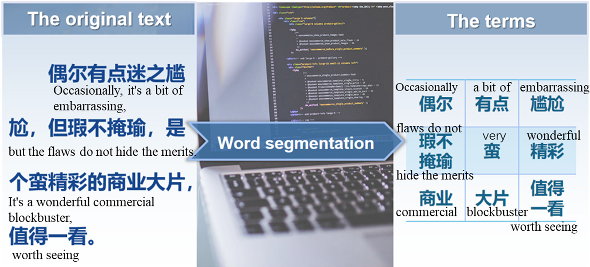
Figure 2: An example of the Chinese word segmentation

3.3 Data Vectorization

In this study, the data is the text downloaded from the website, so data vectorization means text vectorization. Text vectorization consists of two-dimension types: word frequency and semantics. Both have their advantages; this paper has experimented with the two vectors, respectively. Finally, a comprehensive text vector was constructed by combining the two methods and used in the experiments for comparison.

3.3.1 Text Vectorization Based on Word Frequency

The Vector Space Model [31] (VSM) is one of the simplest and most efficient text representation models in the field of text retrieval and text classification. The model is mainly composed of text, terms, and term weights, of which the selection of terms and the calculation of weights are critical processes. The terms generally need to have three characteristics: 1) cover as many text topics as possible, 2) fully reflect the unique content of the text, and 3) the terms should be as independent as possible.

Based on the basic concepts above, the process of text vectorization could be divided into the following steps: 1) Extract all the terms (t1,t2,t3......tn) in text d, 2) calculate the weights of each term separately. Traditional vector space models take the number of occurrences of terms in the text as their weights, and Fig. 3 illustrates a model representation of this approach:

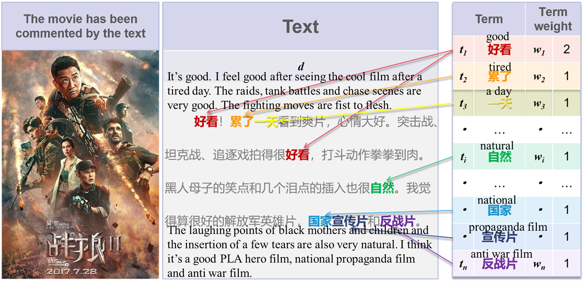
Figure 3: An example of the traditional vector space model

(1) TF-IDF Vector Space Model

However, the traditional vector space model has a disadvantage that it cannot show the rate of the term’s appearance in the text, which can indicate the importance of the term. Therefore, an importance adjustment factor needs to be added to measure whether a word is a common word. If a word is rare in an entire text collection but appears multiple times in a text, it is likely to be a keyword that reflects the characteristics of the text. In this paper, the Term Frequency-Inverse Document Frequency (TF-IDF) vector space model was introduced to adjust the importance coefficient of the terms.

In m text sets (d1,d2,d3......dm), there are n terms (t1,t2,t3......tn). Then the word frequency TFti,dj of the term ti in the text dj is calculated by Eq. (2):

TFti,dj=fti,djldj(2)

where fti,dj is the number of times ti appears in dj, and is the total number of occurrences of all terms in dj. The inverse document word frequency of the term T in the text set is calculated by Eq. (3):

IDFti=log2(mmti¯+1)(3)

where m represents the total number of texts in the text set, and mti¯ represents the total number of texts in the text set containing the term ti. The denominator is incremented by 1 to avoid calculation errors caused when mti¯ is 0. The weight of term ti in text dj is calculated by Eq. (4):

TF−IDFti,dj=TFti,dj×IDFti=fti,djIdj×log2⁡(mmti¯+1)(4)

In this paper, the improved vector space model was used to create the text word frequency vector for the data samples, which was used as the input of the classification neural network.

(2) PCA-Based Text Vector Dimensionality Reduction

For the previously obtained word-frequency matrix, a dimensional explosion likely occurred due to the large dimensionality, so the dimension of the text vector needs to be reduced. To reduce the vector dimension, this paper used the principal component analysis [18] method (hereinafter referred to as PCA).

The theoretical basis of PCA is mainly the theory of maximum variance. For example, a document vector has n features, and now you need to map it to another k-dimensional space, where k < n. To preserve the differences in the k-dimensional text vectors obtained after mapping as much as possible, the sample variance of each dimension needs to be as large as possible, as shown in Figs. 4a and 4b.

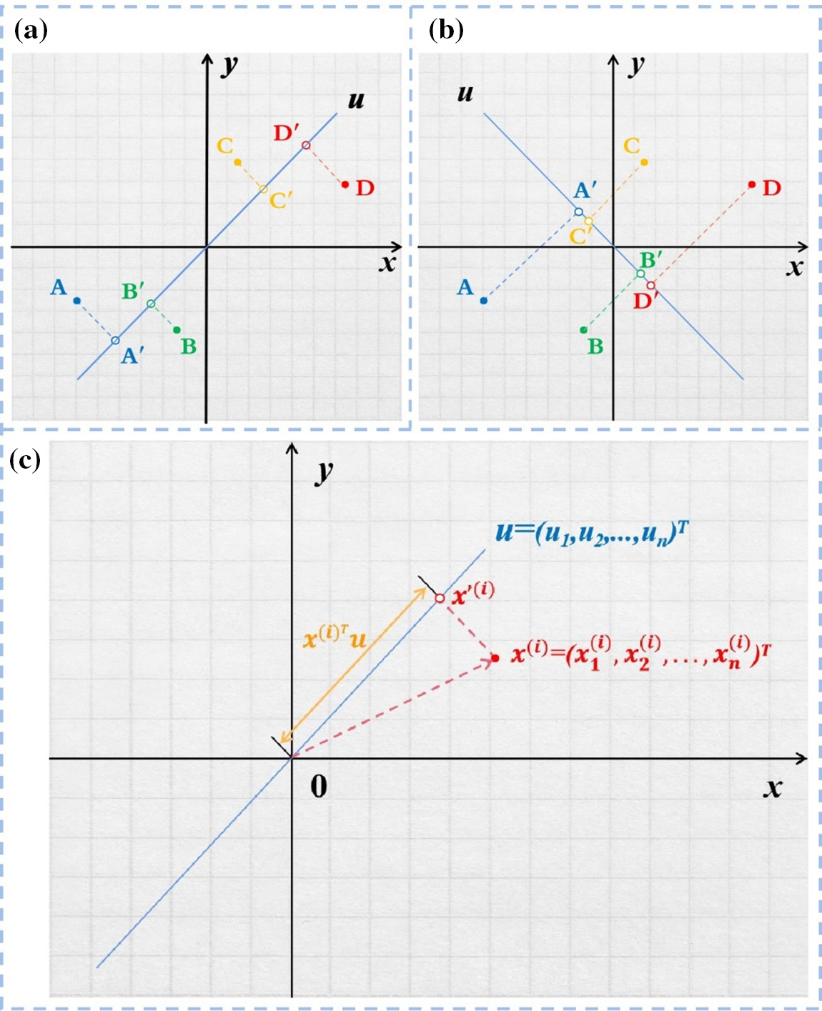
Figure 4: A diagram of vector dimensionality reduction and mapping with PCA. (a) and (b) show the vector dimensionality reduction, there are two kinds of mappings of points A, B, C, and D in two-dimensional space to points in one-dimensional space, A′, B′, C′, D′, and the method that (a) shows is better for preserving the differences. (c) is the PCA mapping mode

In Fig. 4c, the point x(i) represents a point in n-dimensional space, and the point x′(i) represents the projection of the point x(i) on u, u is the unit direction vector of the line. The distance of point x′(i) to the origin (“0”) is x(i)Tu. To find the best vector u, it is necessary to have the maximum variance projected on the u for all sample points in m sample points, that is, to get the maximum value to the left of the equal sign of Eq. (5):

1m∑i=1m(x(i)Tu)2=1m∑i=1muTx(i)x(i)Tu=uT(1m∑i=1mx(i)x(i)T)u(5)

In the equation above, 1m∑i=1mx(i)x(i)T is the covariance matrix of point x(i). We use λ to denote 1m∑i=1m(x(i)T)2, and use ∑ to denote 1m∑i=1mx(i)x(i)T, then the equation above can be written as λ=uTΣu.

For u is a unit vector, uTu=1, both sides of λ=uTΣu multiplied by u at the left and get the equation uλ=Σu, λ is a real number, so it can be written as Σu=λu. It can be seen that λ is the eigenvalue of the Σ, and u is the eigenvector corresponding to the eigenvalue λ. Using the eigenvalue decomposition method to manipulate the covariance matrix Σ, the first k large eigenvalues obtained are the eigenvalues we need, and the eigenvectors corresponding to these k eigenvalues are the k-dimensional new features that we need to obtain. After obtaining the first k eigenvectors u, using the formula (6) converts x(i) to x′(i):

x′(i)=[u1Tx(i)u2Tx(i)⋮ukTx(i)](6)

In the formula, ujTx(i) is the projection of x(i) on uj, the terms with minor variances can be eliminated using this method.

(3) Accuracy Measuring

Accuracy is used in this paper to measure experimental results. Assume that the actual and predicted classification results are shown in Table 1:

The accuracy could be calculated using Eq. (7):

accuracy=TP+TNTP+TN+FP+FN(7)

3.3.2 Text Vectorization Based on Semantics

The Continuous Bag of Words Model (CBOW) is a way to train word vectors. Word2vec is a simple and efficient representation of word vectors based on CBOW proposed by the Google team. The doc2vec model is proposed based on the Word2vec model. Doc2vec has two kinds of models, which are distributed Memory Model of Paragraph Vectors (PV-DM) and distributed Bag of Words version of Paragraph Vector (PV-DBOW). This paper uses the PV-DM model in Fig. 5 to train the obtained text vector.

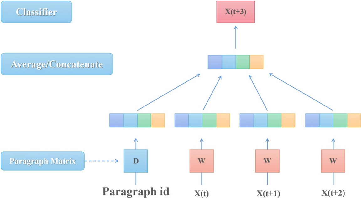
Figure 5: The structure of the PV-DM model

In the PV-DM model, the input layer is constructed by W and D together. Assuming that there are m texts, the total number of words is set to n, and the number of hidden layer nodes (the dimension of the desired text vector) is k, then the size of matrix D is m × k, and the size of matrix W is n × k. Each row vector of matrix D is the text vector of the corresponding id, and each row vector in matrix W is the word vector of each word.

The hidden layer not only operates on all word vectors but also adds the text vector corresponding to the id, and the text vector and word vector predict the next word in the context by averaging or stitching them together. Different texts have different text vectors, but the exact words in different texts have the same word vectors.

When using the PV-DM model to train a document vector, the word vector is also trained with an excellent performance in the meaning of the word, and it can easily find words that are similar in the meaning of a word or words that are very relevant. In this paper, the document vector obtained by using the above method is called a text semantic vector.

3.3.3 Calculation of the Value Degree of Text

Internet “water army” create hot spots by making false comments, which look real but are often similar in structure and have a particular emotional bias. Therefore, this paper proposes to calculate the “value degree” for the comment text based on these two characteristics, further improving the accuracy of the model.

(1) Calculate text similarity based on structure encoding and word frequency

•   Calculate text similarity based on structure encoding

Before calculating the similarity, the text structure encoding should be built. First, useless information was excluded from the text, such as spaces, special characters, and punctuation marks. Then the stuttering participle was used to segment it, and the part of speech of each word was obtained. According to the part of speech, the noun, verb, adjective, number, quantifier, pronoun, adverb, preposition, conjunction, auxiliary and other words was calibrated in order as 1, 2, 3, 4, 5, 6, 7, 8, 9, 10, 11. Then a structural coding vector was obtained. As shown in Fig. 6:

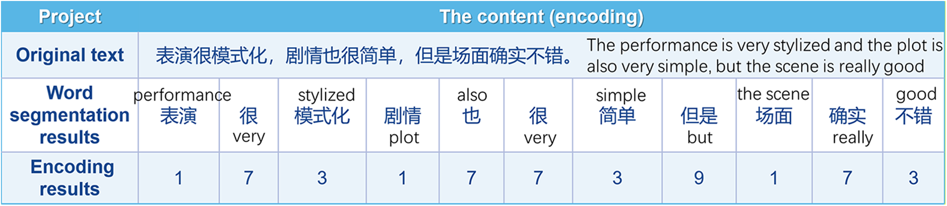
Figure 6: Diagram of text structure encoding

Suppose that the structure encoding vectors of text ti and tj are di and dj. The structural similarity SSim(ti,tj) between them can be measured by the Jaccard coefficient, using the formula (8):

SSim(ti,tj)=|di∩dj||di|+|dj|−|di∩dj|(8)

The length of the longest common subsequence of text vectors di and dj was represented by |di∩dj|, and the length of di was represented by |di|, so as |dj| to dj.

•   Calculate text similarity based on word frequency

After word-segmentation and deleting the deactivation words, text ti and tj produced a set of k terms {f1,f2,f3…fk}. Construct a text word frequency vector from a collection of terms, respectively:

Vti=(wi,1,wi,2,……wi,k)(9)

Vtj=(wj,1,wj,2,……wj,k)(10)

In the collections, wi,k is the number of occurrences of fk in ti, and wj,k is the number of occurrences of fk in tj. The cosine coefficients shown in Formula (3)–(5) have been used for similarity measuring of text ti and tj:

FSim(ti,tj)=∑n=1kwi,n∗wj,n(∑n=1kwi,n2)(∑n=1kwj,n2)(11)

•   Calculate the synthetic similarity

The two similarities of (1) and (2) were combined to obtain a comprehensive similarity Sim(ti,tj), and the calculation formula is as follows:

Sim(ti,tj)=ω1∗SSim(ti,tj)+ω2∗FSim(ti,tj)(ω1+ω2=1,ω1>=0,ω2>=0)(12)

In the formula, ω1 and ω2 could be selected according to the specific sample, this paper sets ω1=0.3, because the structural coding similarity introduced in this study is only to increase the similarity between a small part of the text, and does not have much impact on the whole text.

(2) Text sentiment analysis based on the sentiment dictionary

This paper has conducted text sentiment analysis based on the emotion dictionary: 1) A network emotion dictionary was constructed to combine with the existing emotion dictionary. 2) A set of negative words was created, and its weight was set to −1. 3) A degree adverb dictionary was constructed, degree adverbs were classified into four categories: extreme, high, medium, and low, and the weights of each category of degree adverbs were set. 4) The emotional tendency was calculated; the method of calculation is as follows:

For the text ti, firstly, the punctuation symbol was used as its separator, and text ti was divided into n sentences S1, S2, S3...Sn. In Si, the number Si,n of negative words, the weight Si,d of the emotional degree adverb, and the weight Si,a of the emotional word were sequentially selected. The sentimental bias weight of the sentence Si was a comprehensive calculation of the negative word ESi, the emotional degree adverb, and the emotional word, which was calculated by the formula (13):

ESi=(−1)Si,n∗Si,d∗Si,a(13)

The emotional tendency value Eti of the text ti was the sentimental bias weight of the sentences S1, S2, S3...Sn, and is calculated by Eq. (14):

Eti=∑i=1nESi(14)

The emotional tendency value Eti of the text ti finally obtained according to the above formula was divided into three different ranges, when Eti>0, it was divided into positive emotions; when Eti=0, it was divided into neutral emotions; when Eti<0, it was divided into negative emotions.

(3) Calculate the value of the text based on similarity and sentiment

In m text samples, the similarity Sim(ti,tj) between them can be calculated between any two texts ti and tj. For any text ti, the similarity between it and other m-1 samples can be calculated. By averaging the m–1 similarities, the overall similarity ASim(ti) of the text ti can be obtained, and the calculation formula is as follows:

ASim(ti)=1m−1∑k=1,k≠imSim(ti,tk)=1m−1(∑k=1mSim(ti,tk)−Sim(ti,ti))

=1m−1(∑k=1mSim(ti,tk)−1)(15)

The ASim(ti) calculated by the above formula has a value between 0 and 1. The closer this value is to 1, the greater the similarity between the text ti and the other samples, indicating that the value of the text is lower.

If the emotional tendency value Eti of text ti is too big or too small, both indicate that the emotional tendencies of text ti are too extreme, and its value needs to be reduced.

In m text samples, the emotional propensity value of each sample can separately be obtained, and be divided into two categories according to greater than 0 or less than 0. The average value E+¯ and E−¯ was calculated respectively by the following (16):

E+¯=∑k=1mEtk(Etk>0),E−¯=∑k=1mEtk(Etk<0)(16)

This paper considered the emotional propensity value of a text with an emotional tendency value between E−¯ and E+¯, which did not affect the calculation of its value. In the text whose sentiment tendency value is outside the interval, the closer the emotional tendency value is to both ends, the lower the value Vati is, as shown in Fig. 7 below.

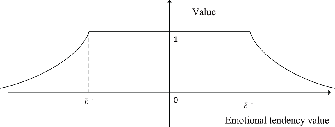
Figure 7: Relationship between text value and sentiment orientation value

Vati={E−¯/Eti(Eti<E−¯)1(E−¯<=Eti<=E+¯)E+¯/Eti(E+¯<Eti)(17)

For text ti, its text value is composed of two parts. The first part is the similarity obtained. The greater the similarity, the lower the value. The second part is the value of emotional tendency. The text value Valti combining the similarity with emotion was calculated according to the following formula. The value of α1 in this experiment was set to 0.5.

Valti=α1∗(1−ASim(ti))+α2∗Vati(α1+α2=1,α1>=0,α2>=0)(18)

3.4 Module Building

In this study, a multilayer BP neural network was used for experiments, and multiple sets of experiments were performed on different hyperparameters to obtain the best model. The structure of the neural network is shown in Fig. 8:

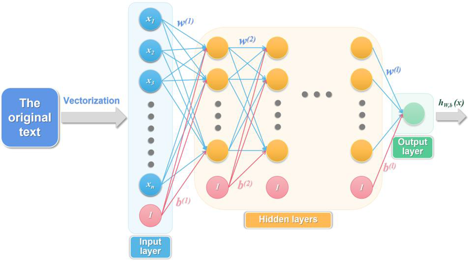
Figure 8: The structure of the text filtering model based on the BP neural network

In this model, the original text should be vectorized at the beginning, x1,x2,x3......xn and 1 together make up the input layer of the neural network, the rightmost layer is the output layer of the neural network (in this case, the output layer has only one node), and all the nodes in the middle together make up the hidden layer of the neural network.

The number of input layer nodes is determined by the dimension after the text vectorization, the number of hidden layers was set to 0 to 5 in turn, and the number of hidden layer nodes was determined using the empirical formula (19):

h=m+n+a(19)

In the formula, the number of hidden layer nodes is expressed by h, the number of input layer nodes is expressed by m, the number of output layer nodes is expressed by n, and a is a parameter that can be adjusted according to the specific application scenario, and its range is 1–10.

4  Results and Discussion

In this paper, we test the effect of dimensionality reduction processing of data, and study the methods of word frequency vector and semantic vector, to find a more effective text vectorization method.

4.1 Effects of PCA Dimensionality Reduction

A text word frequency vector was created for the 40,000 comment samples filtered in the previous part of this paper using TF-IDF vector space model, and a matrix of 40,000 × 10,930 was obtained. However, such a term dimension is still too large and requires dimensionality reduction by the PCA method, solving the problem of sparse vectors and large dimensions. This study tests the relationship between the principal component retention scale and the vector dimension, and the results are as shown in Fig. 9 and Table 2:

Figure 9: Relationship between principal component retention ratio and vector dimension

As shown in the figure above, when the vector dimension drops to 5981, it is still possible to retain 95% of the principal component ratio. Therefore, PCA dimensionality reduction can not only preserve text features as much as possible but also greatly reduce the amount of computation.

Through experiments, the optimal proportion of principal component retention was 90%, and the vector dimension of word frequency was 4371 after dimension reduction.

4.2 Word Frequency Vectors

After the data was reduced in dimension, we conducted two steps of experiments to confirm the accuracy of the word frequency vector: 1) to fix the number of hidden layers, and test the dimension of different text word frequency vectors, 2) to fix the dimension with the best result, and measure the number of different hidden layers to determine the optimal effect.

First, different dimensional text vectors after PCA dimensionality reduction were tested on models with only one hidden layer, the number of hidden layer nodes was calculated according to the formula h=m+n+a, where a was set to 4 (All of the subsequent experiments use this setting). Experiment with different models using different iterations to get the highest accuracy for each dimension, and then compare them. The results are as Fig. 10a, it can be seen that with the decrease of the word frequency text vector, the accuracy of the model showed a trend of improvement at the beginning, and a decreasing trend occurs in the second half. The accuracy of the model was the best in the 4371 dimensions (90% of the principal components were retained).

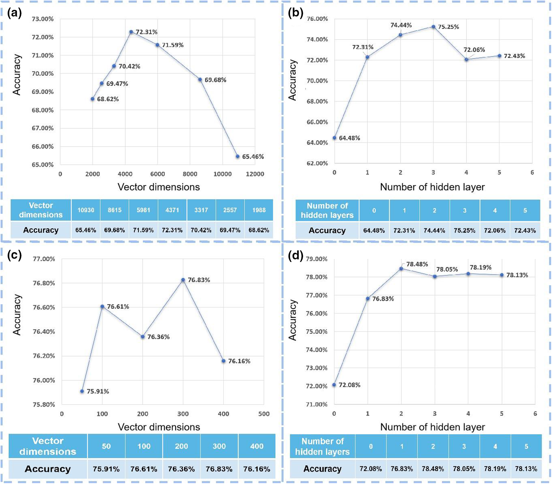
Figure 10: The text vectors and their accuracies. (a) Relationship between vector dimensions and accuracy of word frequency vectors. (b) Relationship between the number of hidden layers and accuracy of word frequency vectors. (c) Relationship between vector dimensions and accuracy of text semantic vectors. (d) Relationship between the number of hidden layer and accuracy of text semantic vectors

Then, using the text word frequency vector of the 4371 dimensions, test the model of different hidden layers, calculate the number of hidden layer nodes to 70, and set the number of hidden nodes of each hidden layer to be the same. Different models also experimented with different iterations, and the highest accuracy of each hidden layer was obtained as the final experimental comparison value. Fig. 10b shows the result when the number of hidden layers was set to 3, the model can achieve the optimal effect, and the prediction accuracy is nearly 3 percentage points higher than that of a single hidden layer.

4.3 Text Semantic Vectors

To make the vector representation contain rich text semantic information, the PV-DM model was used to train the collected 40,000 comment data. The window size was set to 3, which means predicting the probability of the word according to the 3 words ahead and the 3 words behind, the PV-DM model was used to train the word vector and text vector.

The number of hidden layers was set to 1, and the dimensions of the text vector were set to 50, 100, 200, 300, and 400 respectively, and also obtain the best correct rate for each experiment after different iterations. The experimental results were shown in Fig. 10c, it can be seen from the above experimental results that the dimension of the text semantic vector does not have much influence on the accuracy, and the difference in performance between 100 and 300 is only 0.22%. Through experiments, the optimal dimension of the text semantic vector was 300.

A text semantic vector of 300 dimensions was tested on the model with different hidden layers, and the number of hidden layer nodes was calculated to be 21, and the number of hidden nodes in each hidden layer was set to be the same. Different models also experimented with different iterations, and the highest accuracy of each hidden layer was obtained as the final experimental comparison value. The results show that when the number of hidden layers was set to 2, the model can achieve the optimal effect, and then continue to increase the number of hidden layers, the effect does not change much, as seen in Fig. 10d. When classifying text based on text semantic vectors, the effect was slightly better than that of text word frequency vectors, and the whole model was relatively improved by 3.23%.

4.4 Synthetic Text Vectors

In the next step, the text similarity and sentiment orientation were introduced, and according to the particularity of Chinese text, the “structural coding” of the text is proposed. Then, the text similarity is calculated according to the word frequency similarity and the structural coding similarity, and meanwhile, the sentiment orientation value is calculated for the text based on the sentiment dictionary method. Finally, the text value is calculated by combining the text similarity and the sentiment orientation value.

Based on the previous experiment, when the hidden layers were set to 3, the model always with good performance, so the number of hidden layers was set to 3, and the number of nodes of each hidden layer was the same. The experiment shows that the effect of combining the semantic vector with the word frequency vector that has been reduced dimensionality by the PCA method was better than the other combination, as shown in Fig. 11:

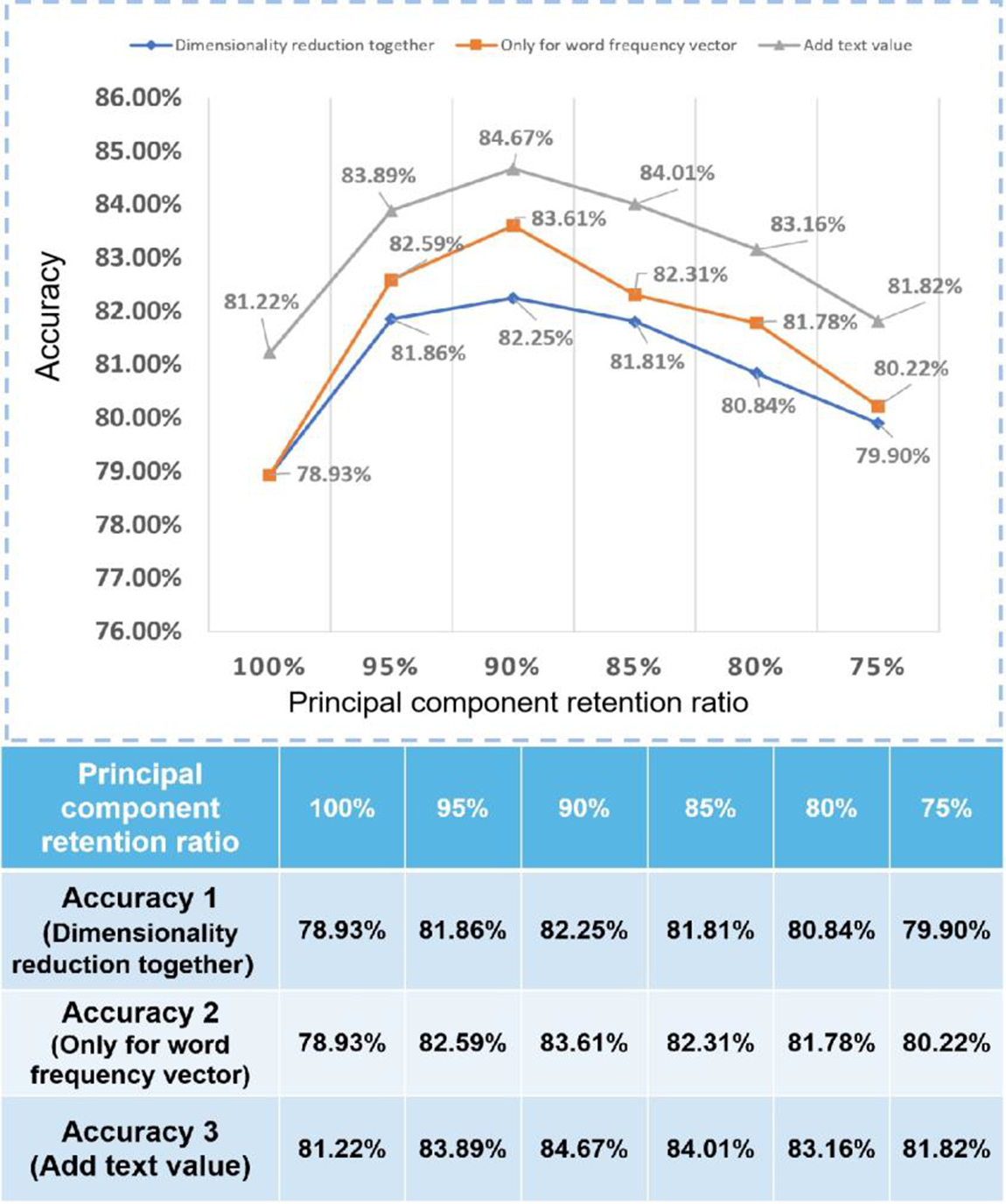
Figure 11: Comparison of 3 text vector combination methods

The results show that the highest accuracy rate was 83.61% when the word frequency vector is dimensionally reduced. And when experiments combined the original text word frequency vector with the semantic vector, the results show that the accuracy was significantly higher than 75.25% when the word frequency vector was used alone and 78.48% when the semantic vector is used alone.

As shown in Fig. 11, accuracy 2 was better than accuracy 1. This is because if the PCA dimensionality reduction processing was performed on both the text word frequency vector and the text semantic vector, the text semantic vector was relatively dense, so it will account for a relatively large proportion of it, resulting in the loss of some text word frequency vector components. Accuracy 3 was the best model and achieved the highest precision (84.67%) during the experiment. The experimental results show that the accuracy of the whole model was increased by 1.06% after adding value, which has little effect on the computational efficiency of the model. The ratio of improvement was not particularly high with only one dimension to the input of the model.

From the above experiments, the model with the highest accuracy was shown in the following Fig. 12:

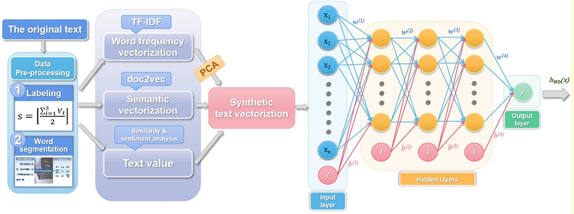
Figure 12: The model with the highest accuracy

5  Conclusion

A high-precision text classification model is designed for text filtering, and the manually calibrated review data of the Douban movie website is selected for research. Firstly, a text filtering model based on BP neural network is established; Secondly, TF-IDF and doc2vec methods are used to obtain the text word frequency vector and text semantic vector respectively, and PCA is used to linearly reduce the text word frequency vector. Finally, the reduced dimension word frequency vector is combined with the text semantic vector, and the text value degree is added to construct the text synthesis vector. Experiments show that the model has reached the highest accuracy of 84.67%.

In the research process, the following research directions can be found:

First, it is possible to try to use a circular neural network to build a model to mine more effectively the relationship between the former part and the latter part of the input.

Second, in the construction of text vectors, more tags can be added to word frequency vectors and semantic vectors to improve the filtering accuracy.

Third, the current popular network language does not exist in the basic emotion dictionary, but it dramatically impacts emotional orientation judgment. Therefore, it is necessary to construct a network emotion dictionary based on the existing emotion dictionary.

What’s more, the selection of the corpus needs to be improved. Due to the limitation of computer performance, the data set has yet to be selected as too large. Later, more large-scale training can be carried out on the cloud server. At the same time, there will be more or less human factors in the sample calibration process. Later, unsupervised learning methods would be considered to use for text classification.

Last but not least, there are few pieces of research on processing at the character level for Chinese text. Character-based processing can be further improved in theory with more text information if there is a good learning model or method. The follow-up of the accuracy of the model will be studied at the character level.

Funding Statement: Supported by the Sichuan Science and Technology Program (2021YFQ0003).

Availability of Data and Materials: The datasets have been analyzed in this study were downloaded from the “Douban movie” website. The data URLs: (https://movie.douban.com/subject/26363254/comments?status=P).

Conflicts of Interest: The authors declare that they have no conflicts of interest to report regarding the present study.

References

1. C. Xu, B. Yang, F. P. Guo, W. F. Zheng and P. Poignet, “Sparse-view CBCT reconstruction via weighted Schatten p-norm minimization,” Optics Express, vol. 28, no. 24, pp. 35469–35482, 2020. [Google Scholar] [PubMed]

2. S. Liu, X. Wei, W. Zheng and B. Yang, “A four-channel time domain passivity approach for bilateral teleoperator,” in 2018 IEEE Int. Conf. on Mechatronics and Automation (ICMA), Changchun, China, pp. 318–322, 2018. [Google Scholar]

3. B. Yang, X. Y. Peng, W. F. Zheng and S. Liu, “Optimal orthogonal subband fusion for online power system frequency estimation,” Electronics Letters, vol. 52, no. 5, pp. 390–391, 2016. [Google Scholar]

4. B. Yang, C. Liu and W. F. Zheng, “PCA-based 3D pose modeling for beating heart tracking,” in 2017 13th Int. Conf. on Natural Computation, Fuzzy Systems and Knowledge Discovery (ICNC-FSKD), Guilin, Peoples R. China, pp. 586–590, 2017. [Google Scholar]

5. Y. Liu, W. Gan and Q. Zhang, “Decision-making mechanism of online retailer based on additional online comments of consumers,” Journal of Retailing and Consumer Services, vol. 59, no. 1, pp. 102389, 2021. [Google Scholar]

6. B. Zhu, D. Guo and L. Ren, “Consumer preference analysis based on text comments and ratings: A multi-attribute decision-making perspective,” Information & Management, vol. 59, no. 3, pp. 103626. [Google Scholar]

7. A. G. Mauri and R. Minazzi, “Web reviews influence on expectations and purchasing intentions of hotel potential customers,” International Journal of Hospitality Management, vol. 34, no. 1, pp. 99–107, 2013. [Google Scholar]

8. M. C. and X. Jin, “What do airbnb users care about? An analysis of online review comments,” International Journal of Hospitality Management, vol. 76, no. 2, pp. 58–70, 2019. [Google Scholar]

9. T. Chen, L. Peng, J. Yang and G. Cong, “Analysis of user needs on downloading behavior of english vocabulary APPs based on data mining for online comments,” Mathematics, vol. 9, no. 12, pp. 1341, 2021. [Google Scholar]

10. X. Gao and Q. Liu, “Dynamics and evaluations of impoliteness: Evidence from short videos of passenger disputes and public comments,” Journal of Pragmatics, vol. 203, no. 2, pp. 32–45, 2023. [Google Scholar]

11. S. Kohout, S. Kruikemeier and B. N. Bakker, “May I have your attention, please? An eye tracking study on emotional social media comments,” Computers in Human Behavior, vol. 139, no. 5, pp. 107495, 2023. [Google Scholar]

12. J. C. -T. Ho, “How biased is the sample? Reverse engineering the ranking algorithm of Facebook’s graph application programming interface,” Big Data & Society, vol. 7, no. 1, Article number 205395172090587, 2020. [Google Scholar]

13. H. Allcott and M. Gentzkow, “Social media and fake news in the 2016 election,” The Journal of Economic Perspectives, vol. 31, no. 2, pp. 211–236, 2017. [Google Scholar]

14. B. Yang, T. Cao and W. Zheng, “Beating heart motion prediction using iterative optimal sine filtering,” in 2017 10th Int. Congress on Image and Signal Processing, BioMedical Engineering and Informatics (CISP-BMEI), Shanghai, China, pp. 1–5, 2017. [Google Scholar]

15. E. Humprecht, L. Hellmueller and J. A. Lischka, “Hostile emotions in news comments: A cross-national analysis of Facebook discussions,” Social Media+ Society, vol. 6, no. 1, Article number 2056305120912481, 2020. [Google Scholar]

16. D. M. J. Lazer, M. Baum, Y. Benkler, A. J. Berinsky, K. M. Greenhill et al., “The science of fake news,” Science, vol. 359, no. 6380, pp. 1094–1096, 2018. [Google Scholar] [PubMed]

17. Pew Research Center, “Many Americans believe fake news is sowing confusion,” 2016. [Google Scholar]

18. M. Ziegele, Nutzerkommentare als Anschlusskommunikation: Theorie und qualitative Analyse des Diskussionswerts von Online-Nachrichten, Wiesbaden: Springer VS, 2016. [Google Scholar]

19. S. G. Winster and M. N. Kumar, “Automatic classification of emotions in news articles through ensemble decision tree classification techniques,” Journal of Ambient Intelligence and Humanized Computing, vol. 12, no. 5, pp. 5709–5720, 2021. [Google Scholar]

20. D. Metzler, S. Dumais and C. Meek, “Similarity measures for short segments of text,” in European Conf. on Information Retrieval Springer, Berlin, Heidelberg, pp. 16–27, 2007. [Google Scholar]

21. A. Maas, R. Daly, P. T. Pham, D. Huang and C. Potts, “Learning word vectors for sentiment analysis,” in Proc. of the 49th Annual Meeting of the Association for Computational Linguistics: Human Language Technologies, Portland, Oregon, USA, pp. 142–150, 2011. [Google Scholar]

22. F. Sebastiani, “Machine learning in automated text categorization,” Acm Computing Surveys, vol. 34, no. 1, pp. 1–47. [Google Scholar]

23. Y. Ma and S. Lin, “Application of LDA-LR in personalized news recommendation system,” in 2018 IEEE 9th Int. Conf. on Software Engineering and Service Science (ICSESS), China Hall Sci & Technol., Beijing, Peoples R. China, pp. 279–282, 2018. [Google Scholar]

24. Q. Zhou, Y. Liu, Y. Wei, W. Wang, B. Wang et al., “Dirichlet process mixtures model based on variational inference for Chinese person name disambiguation,” in Proc. of the 2018 Int. Conf. on Computing and Data Engineering, New York, NY, USA, pp. 6–10, 2018. [Google Scholar]

25. T. Mikolov, K. Chen, G. Corrado and J. Dean, “Efficient estimation of word representations in vector space,” in Int. Conf. on Learning Representations, Scottsdale, Arizona, 2013. [Google Scholar]

26. Q. V. Le and T. Mikolov, “Distributed representations of sentences and documents,” in Int. Conf. on Machine Learning, PMLR, Bejing, Peoples R. China, 2014. [Google Scholar]

27. T. Wolf, L. Debut, V. Sanh, J. Chaumond, C. Delangue et al., “Huggingface’s transformers: State-of-the-art natural language processing,” arXiv preprint, 1910.03771, 2019. [Google Scholar]

28. G. Xu, Z. Yu, H. Yao, F. Li, Y. Meng et al., “Chinese text sentiment analysis based on extended sentiment dictionary,” IEEE Access, vol. 7, pp. 43749–43762, 2019. [Google Scholar]

29. J. Zhang, Y. Zhong, P. Chen and S. Nichele, “Emotion recognition using multi-modal data and machine learning techniques: A tutorial and review,” Information Fusion, vol. 59, no. 1, pp. 103–126, 2020. [Google Scholar]

30. J. A. Fodor and Z. W. Pylyshyn, “Connectionism and cognitive architecture: A critical analysis,” J. Cognition, vol. 28, no. 1–2, pp. 3–71, 1988. [Google Scholar]

31. G. Salton, “A vector space model for automatic indexing,” Communications of the ACM, vol. 18, no. 11, pp. 613–620, 1975. [Google Scholar]