A Robust Approach for Detection and Classification of KOA Based on BILSTM Network

1  Introduction

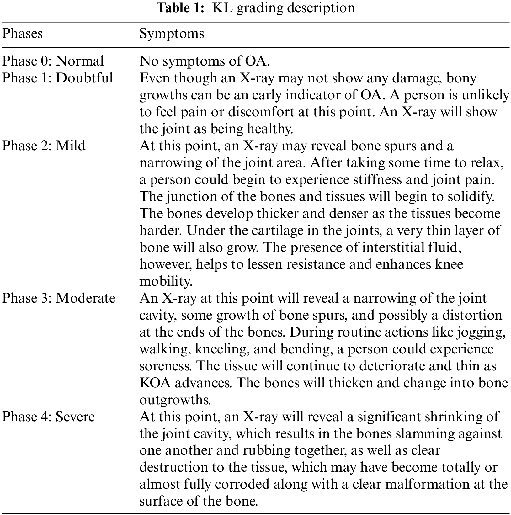
With the increasing population, the patients of with KOA have been continuously increasing [1]. KOA carries enormous socioeconomic implications as it is a major source of morbidity and disability. According to estimates, the cost of arthritis in the United States in 2004 was expected to be $336 billion, or 3% of the country’s GDP, with KOA being the most prevalent type [2]. There are no therapies that significantly enhance the OA illness identification process, and the etiology of OA disease is yet unknown [3]. Wear and tear is a degenerative joint condition that gradually destroys articular cartilage. The busy lifestyle may also affect younger individuals. It is a kind of arthritis that primarily affects adults 50 years of age and older. Additionally, osteoarthritis is a painful, long-term joint condition that mostly impacts the hands, hips, and spine in addition to the knees. Every person’s level of symptom intensity is different, and KOA typically takes years to manifest. The KL Grading system’s evolution is frequently described by physicians or other medical professionals using stages. Below, in Table 1, are explanations of the various KL classification phases.

Wear and strain as well as metabolic changes are also contributing factors to knee OA. Elderly, obesity [3], and past knee injuries [4] are known potential risks for OA. Pain brought on by OA restricts movement and lowers the standard of living. Since OA causes irreparable joint deterioration, the final stage of the illness necessitates complete Knee Replacement (TKR), a costly procedure with a limited life expectancy, particularly for an obese person [4]. A physicians classify KOA by looking at changes in knee X-rays using the KL rating scale. Because bone changes are only visible when OA is advanced, this method may postpone the detection of the disease. In addition toX-rays, additional imaging modalities like Magnetic Resonance Imaging (MRI) can be used to assess OA soft tissue and identify the grade of KOA in conjunction with biomarkers such as cartilage and meniscus degradation [5]. A key indicator of how OA is structurally developing is articular change assessment, which is also used to determine how well a therapy is working. The intra-articular soft tissue structures, including cartilage, may be seen in three dimensions using Mitral Regurgitation (MR), a non-invasive technique. Due to the anatomy and morphology of the knee as well as the nature of MR imaging, it is difficult to acquire precise and repeatable quantitative values from MRI images [6]. Each series of the 3-dimensional (3D) knee MRI must be manually segmented, which might take up to six hours. Additionally, substantial training is frequently required of operators who employ cartilage segmentation software [7], which adds to the time and expense. Therefore, there should be an automated system for KOA detection that can identify the severity of knee OA at early stages that is not easy to assess from the human eye. Moreover, an automated system can reduce human effort, time, and erroneous prediction. Thus, orthopedics can start early treatment and therapies to stop the progression of the disease. Various machine learning deep learning-based techniques [8] have been proposed by researchers for the diagnosis of diseases such as eye disease detection [9], diabetes detection [10], and knee disease detection [11]. There are several types of models for KOA detection based on segmentation or classification for evaluating the knee, which are often categorized into traditional machine learning approaches and deep learning (DL) methods [7,12]. Contrarily, machine learning-based models are less general and need manual feature extraction from pictures, which takes time and extra-human work. To lessen diagnostic uncertainty brought on by manual system issues [13]. Recent researchers have applied deep learning models to the medical sector, including the diagnosis of knee OA [14,15]. Through a series of architectural modifications, the deep learning algorithms are taught by automatically extracting visual characteristics [15,16]. Additionally, because of generalization, deep learning models perform well with unobserved data. The availability of vast archives of clinical and imaging data, such as through the OAI [17], has been a further impetus for the development of deep learning algorithms for KOA diagnosis. By forecasting a disease’s prevalence, intensity, or course as well as a medical result, deep neural networks can also assist medical professionals in making a more accurate diagnosis [12,13]. Additionally, computer-aided methods (such as active contours and B-splines) have been developed to help in cartilage segmentation for MR images [18]. Unfortunately, these approaches are not accurate [19] and reliable enough to find minute cartilage changes [14]. There is still a demand among researchers for a quantification technique that is quick to use, valid, and delicate to modification [20]. Some causes of KOA are shown in Fig. 1. The main contributions of our work are below:

•   To propose a novel KOA disease detector that is easy to execute.

•   To develop a system for early KOA detection that is computationally fast. As most of the existing techniques require various manual feature extraction phases which require time and high computational resources.

•   Our proposed system performs pre-processing and segmentation to focus on the knee joint. Then, it extracts the most representative features using ResNet layers. In the end, the BiLSTM network layers is used that solves the problem of long-term dependency among textual features.

•   To propose a system that effectively solves the problem of class imbalance using ResNet-18.

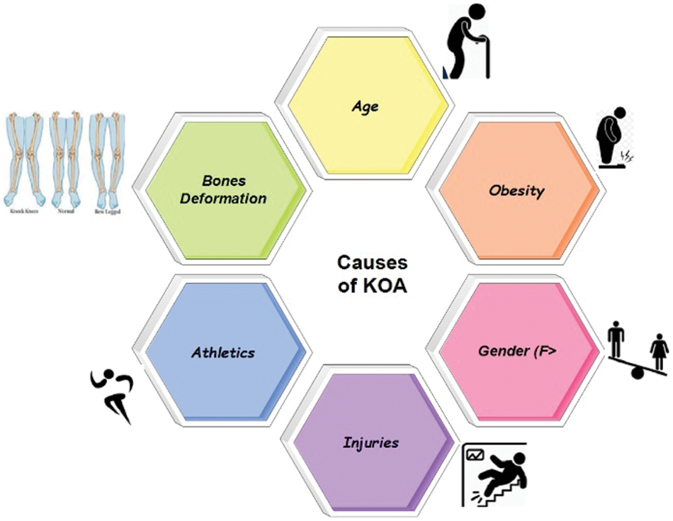
Figure 1: Causes of KOA

2  Related Work

By matching patients who received total TKR with control patients who did not, the authors of [5] devised a convolution (DL) forecast for risk analysis of OA development. The WOMAC (Western Ontario and McMaster Universities Arthritis Index) evaluated the Outcome Score, which was given individually to measure knee symptoms and motions under various activity settings (such as sports and leisure time). Heberden nodes, which are bony enlargements of 1+ distal interphalangeal joints in both hands, family history, a history of a knee injury (difficulty walking for at least a week), and contralateral WOMAC pain score were clinical risk factors [7,12] for KOA. The geometric characteristics between the tibia and femur can be calculated using a distance-based active shape model, which has been established as a tool for KOA diagnosis [21]. To estimate the KL grade from radiographs, ImageNet) [15] and the transfer learning method were both used. Additionally, Guo et al. [15] used a random forest algorithm on clinical factors to predict the 30-month incidence of OA in middle-aged women with a maximal area under the receiver operating characteristic curve AUC of 0.790 for structural KOA development [2]. They suggest using baseline bilateral posteroanterior fixed-flexion knee radiographs to train convolutional neural networks to automatically detect radiographic OA and forecast the evolution of structural OA.

Elderly people have the highest KOA prevalence. The scientists’ completely automated deep learning method, which involves building a convolutional neural network model, is intended to aid in the early diagnosis and treatment of KOA. They avoided the necessity for human picture annotation during both the model’s training and implementation by using data augmentation. The KL score for each image was predicted using a dense convolutional network architecture-based 169-layer convolutional neural network [16] Additionally, similar tasks to KL scoring, where just a tiny section of each overall picture may be significant for class assignments, have also demonstrated the effectiveness of this design in the categorization of orthopedic radiograph, with five outputs total—one for each KL class—the last layer has been adjusted. A pre-trained model on ImageNet and a sizable, annotated database were both utilized to train the model, and the weights of the network were initialized with these weights. The probability for each image corresponding to one of the five KL scores was obtained by applying for a SoftMax nonlinearity role [22] over the five outputs. The model was developed to make predictions with a minimum cross entropy between the OAI committee’s scores and those it had projected.

In [23], authors have proposed a system based on the internet of things to assess the KOA remotely. Their method relied on segmentation and attained 95.23% accuracy for KOA detection however requiring more computational power. In [11], authors have proposed a segmentation-based method for KOA detection. First, they extracted the region of interest and then mined the features using local binary pattern, histogram of oriented gradients, Convolution Neural Network (CNN). In the end, traditional machine learning algorithms such as SVM, K-Nearest Neighbors, and Random Forest have been used. Although the proposed system performed significantly, it was a very lengthy process requiring high computation.

3  Methodology

The process for measuring the severity of knee OA using radiographic images is explained briefly. This approach entails basic stages: pretreatment, extraction of features with CNN, training, and the categorization of knee OA severity with our BILSTM network. The full foundation for early knee OA severity identification is shown in Fig. 2. This study’s main objective is to accurately diagnose early KOA illness and spare patients from having any further operations. Consequently, we have developed a unique technique that combines segmentation and classification to produce results that are more accurate for KOA recognition using the KL rating scale. First, we have employed segmentation on Knee images to attain the region of interest. Second, we extracted the features from those segmented images through ResNet 18. In the end, we utilized our proposed BiLSTM model to classify based on extracted features.

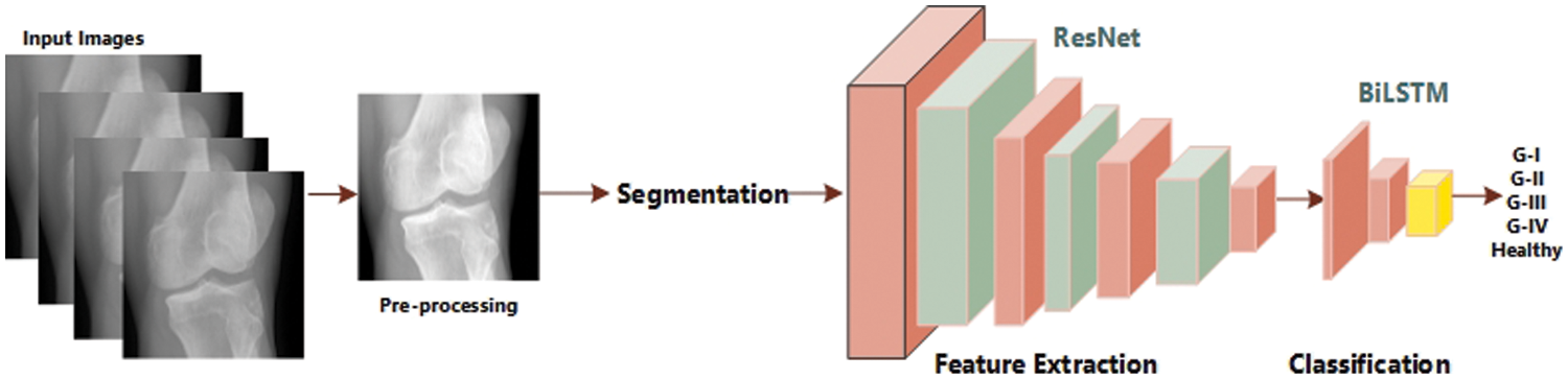
Figure 2: Flow diagram of KOA severity detection

3.1 Data Collection

First, we collected two datasets such as Mendeley Data V1 and OAI [24] for training and cross-validation respectively. We performed various experiments using these two datasets. Mendeley dataset contains about 2000 knee X-ray images having dimensions 224 × 224 × 3. For the OAI dataset, the Multicenter Osteoarthritis Study (MOST) [25,26] and Baltimore Longitudinal Study of Aging (BLSA) [27] conducted a longitudinal, prospective, and observational study of 4,796 people. The categorization in both datasets was made by a radiologist based on the KL [28] measure, which rates the severity of KOA from 0 to 4. Although each patient’s clinical data may be uniquely recognized by an ID, and the medical pictures come from both legs, it is not possible to link them together and follow the patient’s personal information. Additionally, every patient’s privacy was respected. Some sample images from Mendeley data VI are shown in Fig. 3 exhibiting the various grades and healthy. Knees OST [25,26] and BLSA [27] conducted a longitudinal, prospective, and observational study of 4,796 people that looked at KOA.

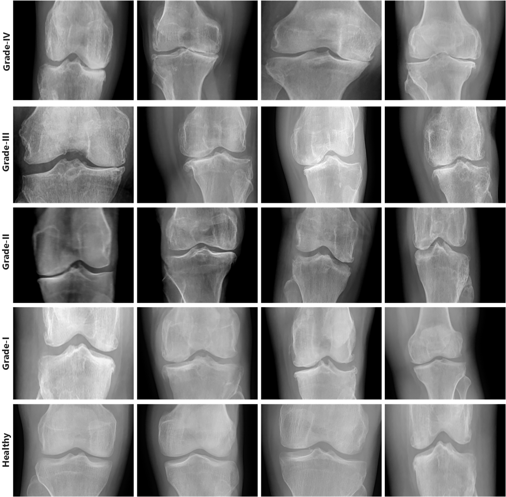
Figure 3: Samples from Mendeley dataset

Our model, which will include knee X-rays and MRIs as well as clinical information about the patient gleaned through private questionnaires, will be trained using the OAI dataset. Our research solely uses data from the baseline assessments, despite the study spanning more than 8 exams over 12 years. As was already noted, the categorization was made by a radiologist and is based on the KL [28] measure, which rates the severity of KOA from 0 to 4. Although each patient’s clinical data may be uniquely recognized by an ID, and the medical pictures come from both legs, it is not possible to link them together and follow the patient’s personal information. Additionally, every patient’s privacy is respected.

3.2 Data Pre-Processing

An image processing phase is required to remove the distortions, and noise, and enhance the features of images. Therefore, in the first phase, we employed image processing operations such as contrast enhancement, background noise removal, rotation, and scaling have been performed on the acquired dataset. We improved the data with two goals in mind: to raise the volume of knee photographs and to mimic what knee images might look like under different settings, such as changing angles and brightness. While rotating the images, the original image does not change, however, the direction may be changed. Moreover, when we enhance the brightness and contrast of knee images, the random intensity improved the view of the knee bone and the gap between the joints. We did not perform pre-processing operations over the knee images as it can cost more computation power for our proposed model.

3.3 Segmentation and Feature Extraction

The grey scale division method divides an image into segments with equivalent statistical characteristics of the simplest and most obvious ways to achieve this is to use the well-known k-means technique, which is an ideal (in terms of least mean squared error) pixel-by-pixel scalar quantization of the image into k levels. K-means type algorithms, which do not impose any spatial limits, may easily be fooled by additive noise. In other words, these algorithms do not consider any knowledge about the connectivity of the segmented picture. Spatial information is generally integrated as a solution to this problem by modeling the image as a Markov Random Field (MRF) or Gibbs Random Field (GRF). The MRF is defined in terms of local qualities, making it difficult to infer a global joint distribution. For this reason, the GRF is more frequently used [29]. Our goal is to increase the a posteriori conditional probability P(x/y) given a segmentation ‘x’ and a data collection ‘y’. A derivation of this kind is necessary for our application as a result. Eq. (1) is provided by Bayes’ theorem.

P(x/y) α P(y/x)P(x)(1)

This equation’s a priori probability for segmentation, P(x), is entirely derived from the random field model. P(y/x) indicates how well the data matches the segmentation as it is. As a result, the segmentation is constrained in opposing ways by these two ideas. While P(x) strives to align the global distribution with the random field’s forecast, P(y/x) looks for the most likely outcome under Gaussian statistics. The final segmentation’s features will depend on how these terms are weighed compared to one another. Fig. 4 shows the example picture both before and after segmentation.

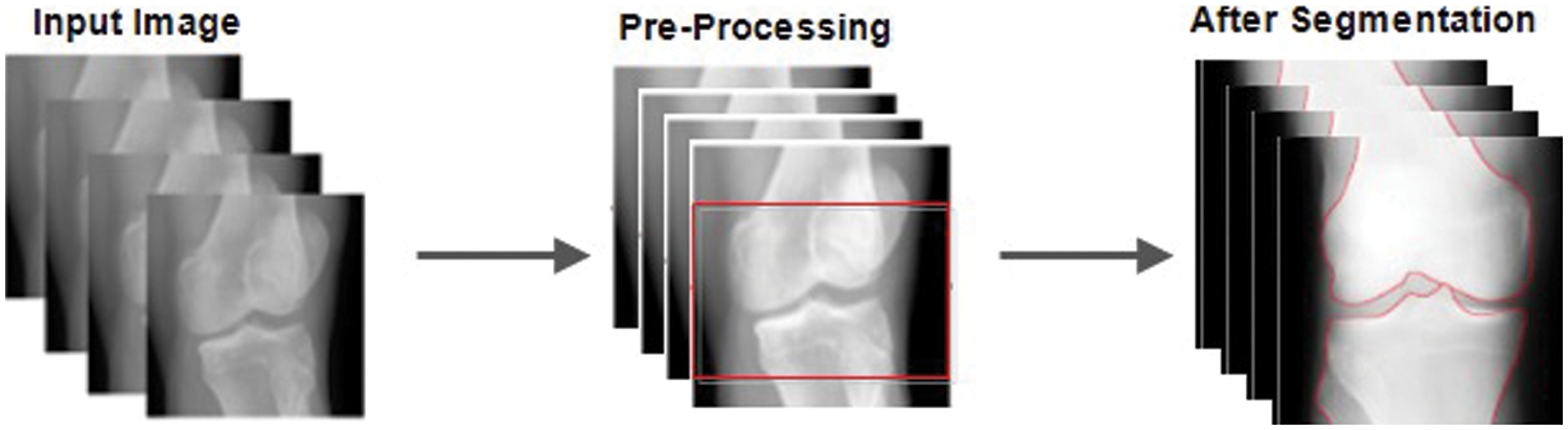
Figure 4: Before and after pre-processing and segmentation

3.4 Convolutional Neural Network

CNN [20] is a deep learning back propagation neural network built primarily for image recognition issues and influenced by biological visual perception. Contrary to typical neural networks, CNN comprises a large number of convolution layers, pooling layers, and the dense layer employing a multi-layered structure to form a deeper network [30,31]. Fig. 5 illustrates how the convolutional neural network’s second layer is fed by the first layer’s output. The core of CNN is its convolutional layer. Each convolution layer consists of several feature maps and a lot of neurons. Utilizing the convolution kernel to scan the image pixel by pixel and extract image attributes, the convolution layer gathers data from neighboring regions in the image. The feature map of the image may be retrieved after turning on the active function. The equation for the operation of convolution is as follows:

Xjl+1=f(∑∈Mjn(Xjl θkijl+1+bil+1))(2)

Figure 5: CNN-structure

Xjl+1 denotes the j-th feature map of the (l+1) th convolution layer, Xjl represents the input Knee images when l=1, f denotes the active function (usually using ReLu function, ReLu = max(x, 0)), M denotes a set of input feature maps, θ denotes a convolution operation, k denotes a convolution kernel, and b denotes an offset term. Pooling the feature map reduces its dimension. Maximum and average pooling are the two mostly used pooling techniques.

3.5 ResNet for Features Extraction

To extract features, we used the Kubkaddi et al. [18] architecture, which is a straightforward and efficient attention-based 2D residual network. Fig. 6 explains the whole design of the Resnet 2D. By extending the depth of the network and addressing the issue of a relatively limited training dataset, the ResNet [18] enhanced the performance of image categorization. We employed the ResNet-18 in particular, which consists of a convolutional layer, eight fundamental ResNet blocks, and a fully connected layer. Two convolutional layers make up each basic block, and each convolutional layer is followed by batch normalization and a nonlinearity activation function called ReLU [18]. In the suggested technique, we used the average-pooling function, which is better suited for illness classification than max-pooling because the average-pooling operation may represent the data on grey matter volume the of brain areas.

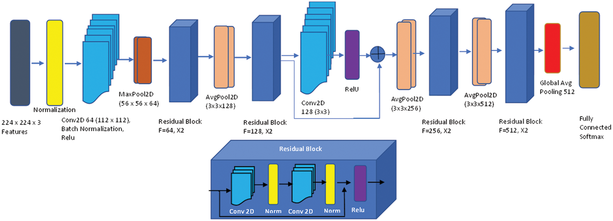
Figure 6: Up: Attention-based ResNet-18; bottom: Residual network block

We used the SoftMax classifier based on cross-entropy loss to the output layer. The attention module is integrated into the ResNet architecture and is executed using just a convolution layer and a set of filters with a kernel size of “3 × 3”. The attention module can capture the significance of different voxels for classification during end-to-end training, which is useful for investigating potential imaging markers. The attention module acts as a feature selector in the forward process. Each voxel of the H × W × D-dimensional extracted features Fi,c is weighted by the H × W × D-dimensional attention mask Mi. The trainable attention mask identifies the importance of each voxel i and is independent of the channel of characteristics and solely relates to spatial location. These are the defined weighted features:

Hi,c=Mi∗Fi,c(3)

where, the spatial position (x, y, z) of the voxel is defined as i(i ∈{ 1,…HxWxD }, x ∈{ 1,…,H } y∈{ 1, …, W }, z∈{ 1,…, D }) and c ∈{ 1,…,C } is the index of the channel. The attention module can also work as a gradient update filter during the back-propagation, therefore, the attention layer makes the network more robust and improves classification performance.

Following end-to-end training, the extension mask automatically improves the possible biomarkers that are crucial for categorization. The attention-based 2D residual network achieves amazing classification performance based on weakly-supervised classification labels (without voxel-wise significant labels), and it also reveals the relevance of prospective biomarkers that may help with illness diagnosis. It is important to note that the custom features may be designed on this end-to-end network without any prior expertise. This network has two advantages: it may help diagnosticians identify possible biomarkers and it is easily adaptable to the categorization of various brain illnesses.

3.6 Classification Using BiLSTM

BiLSTM is a special type of RNN and is the most well-liked network and improved model [32]. It introduces control gate and memory cell technologies to help people memorize information. We preferred the BILSTM network for classification over convolutional neural network layers i.e., fully connected and convolutional layer due to the problem-solving long-term dependency among textual features. By creating the right gate structure and controlling the information flow in the network, BILSTM can store data in complex and sophisticated network elements for a significant length of time. Both remembering the old information network and adjusting the hidden layer settings for the new input network are functions carried out by it. The recurrent neural network layer is divided into four tiers by the structure’s various interactions. By modeling information filtering, remembering crucial information in between sequences, and letting go of irrelevant information, it works out the BiLSTM nerve unit and enables routine information extraction and utilization. The core BiLSTM unit consists of a memory unit and three control gates: input, forget, and output. Its two hidden neural network layers, one in each, have 100 nodes. To explore long-term dependency in the temporal direction, BiLSTM employs these gates. Optimizing BILSTM is made simpler by the gate’s capacity to allow input characteristics to flow through hidden layers without affecting output. Due to its ability to release memory regions in the temporal dimension that do not contribute to the prediction of final classification labels, BILSTM is also able to successfully address the gradient fading problem. The input to BILSTM in this study is the outcome of feature extraction from knee pictures using the Resnet model. After getting model. After getting the features by using DL (Resnet-18) [33] process, we employed the BILSTM transfer learning method, where we customized the sequence to sequence transfer learning model feature input with Bi-LSTM, fully connected, dropout, softmax, and classification layer. We used an input size feature input layer, 02 x Bi-LSTM with 500 and 200 Hidden layers to make it deeper with fully connected consecutive, and also used dropout to overcome the overfitting. The process of applying KL levels 0, 1, 2, 3, or 4 to grade the intensity of knee OA is the last phase. Fig. 7 shows an architecture of BiLSTM network.

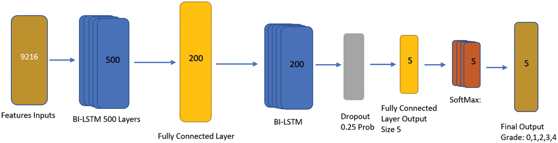
Figure 7: BILSTM proposed architecture

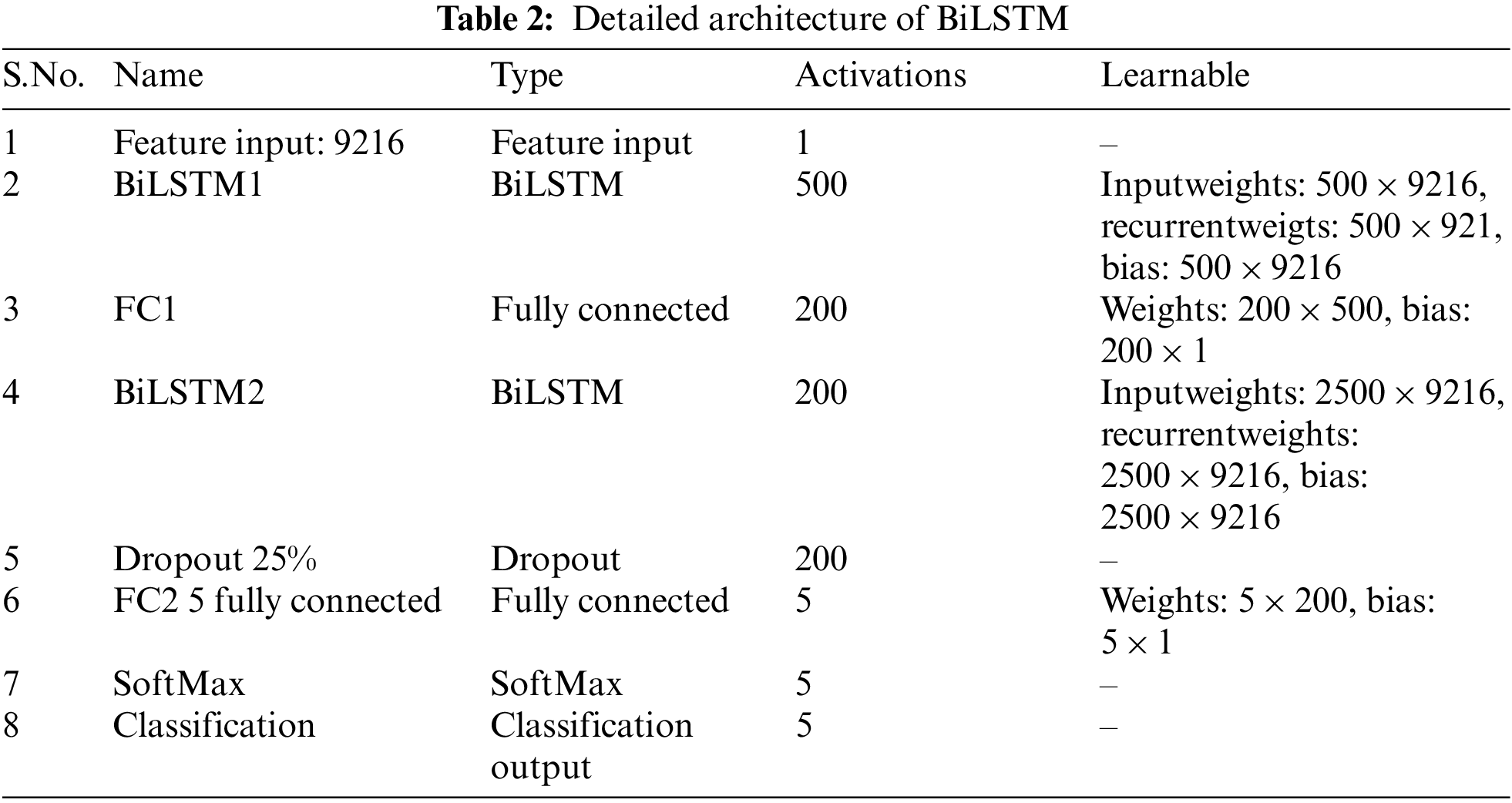
We concentrated on building networks that can categorize knee images with the least amount of learning and validation due to the difficulty of collecting a lot of data from CT scans. The layer’s detail is given in Table 2.

4  Experimental Evaluation

This section summarizes the evaluation findings and provides an analysis of the suggested model. The implementation of the experiment design is represented in part 4.2, and Section 4.1 discusses the dataset in depth. Section 4.3 to 4.5 cover the various trials we conducted to evaluate the effectiveness of the suggested technique.

4.1 Dataset

Here, we go into great depth on the dataset that was utilized for training and testing. Mendeley Data V1 [19] is frequently used for KOA severity identification and categorization using the KL grading scale. Mendeley dataset contains about 2000 knee X-ray images having dimensions 224 × 224 × 3. Two medical professionals have annotated knee images for evaluation to categorize them using the KL grading system. In addition, the pictures were in PNG format and grayscale. The dataset was split into training and validation sets in proportions of 70% and 30%, respectively. More specifically, the model was tested on more than 600 knee photos after being trained on over 1400 knee images. Table 3 reports the Mendeley dataset’s features. We considered Expert-I grading for the distribution of datasets, including 456 healthy class images, 370 grade-I images, 195 grade-II images, 182 grade-III images, and 197 grade-IV images. Fig. 8 displays some examples from the dataset.

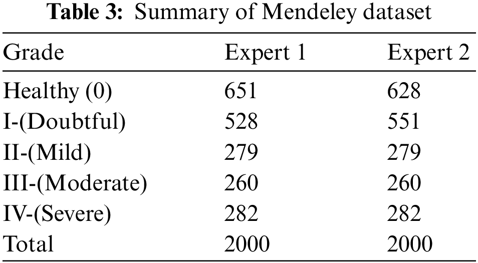
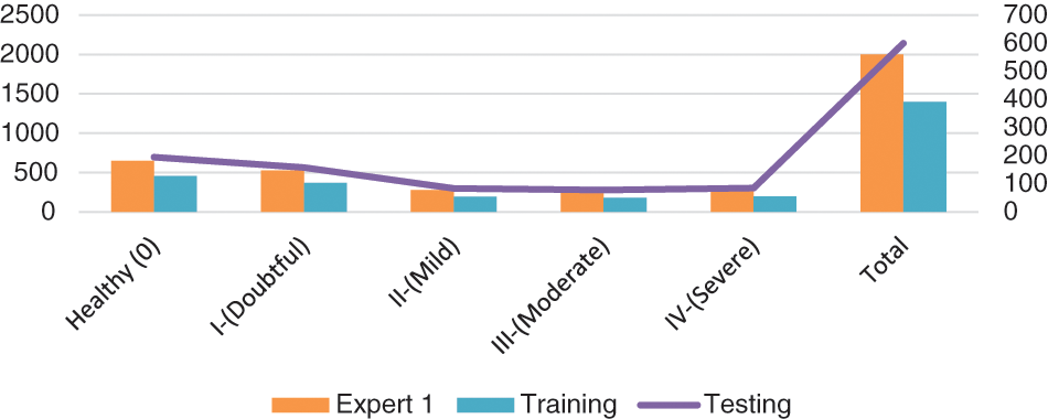
Figure 8: Class-wise distribution of images for training and testing

4.2 Evaluation Setup and Metrics

A Windows-based computer with an Intel(R) Core (TM) i7-8750H processor running at 2.20 GHz, 2208 MHz, with 6 Cores and 12, Logical Processors, and 16 GB of RAM was used for the experiment. NVIDIA GM107GL Quadro K2200/PCIe/SSE2 graphics processing unit. Additionally, the Keres Python framework and library version 2.7 were used to create the suggested model. 60 epochs, 0.00001 learning rate, 35 batch sizes, and stochastic gradient descent were specified as the hyperparameters (SGD). The aforementioned tests were conducted with input image sizes ranging from 32 × 32 by 3 to 64 × 64 by 3 to 224 × 224 by 3. The proposed approach is thought to have performed significantly better than others for an image size of 224 × 224 × 3, nevertheless. The proposed model is assessed using TP, TN, FP, and FN where TP, TN, FP, and FN stand for True Positive, True Negative, False Negative, and False Positive respectively metrics. In other words, the prediction percentage (TP) shows that an image genuinely belongs to that class Grade II and is predicted as Grade II. The possibility that an assessment that a picture does not correspond to a group will be true is measured by TN. For instance, the suggested system could not predict that a leaf is healthy if it does not provide a picture of a damaged leaf. The phrase “FP” refers to the forecasting of the discovery that an image comes from a negative group but is forecasted as not belonging to that class, for instance, if an image contains Grade-III illness and it is forecasted as healthy knee. If an image does not belong to a negative class but is predicted to, i.e., a knee has an illness but is predicted to be healthy, then the image is said to be predicted as belonging to that class.

The confusion matrix that will be used to convey the analysis of the results was built using these four metrics. Depending on how many groups there are, the evaluation procedure will have a [N × N] matrix with the real category on the left-Axes and the anticipated category to an image on the top-Axis. Assume that ′x′  reflect the actual category and that ′y′ reflects the projected category. Below, where ′M′ stands for the matrix, are the confusion metrics components for each class.

TPx=Mxx(4)

FPx=∑i=1nMix−TPx(5)

FNx=∑i=1nMxi−TPx(6)

TNx=∑i=1n∑j=1nMij−TPx−FPx−FNx(7)

Additionally, the four approaches for measuring accuracy—accuracy, precision, recall, and F1 score—are utilized to assess categorization performance. The number of accurate predictions made using the suggested model is represented by accuracy. It is calculated by dividing the total number of predictions made with the proposed system by the number of accurate forecasts. The proportion of photos that are correctly classified by the suggested approach is known as precision. The proportion of the actual number of positive group pictures to the total number of positive category pictures forecasted by the proposed methodology is used to compute it. The percentage of sick images that the system was able to recognize is known as Recall. It is calculated as the percentage of all positive cases that the suggested system successfully classified out of all the positive photos. The F1 score illustrates the performance of the recommended model on the dataset. It is computed using the harmonic mean of recall and accuracy. It shows how reliable the classifier is. The following is a description of the mathematical formulas for the aforementioned metrics.

Accuracy=TP+TNTP+TN+FP+FN,(8)

Precision=TPTP+FP ,(9)

Recall=TPTP+FN,(10)

F1 score=2∗ Precision∗RecallPrecision+Recall,(11)

As a result, Table 4 shows that the suggested approach was able to categorize the knee images into five categories—Healthy, Phase I, Phase II, Phase III, and Phase IV—with an overall accuracy of 84.09 percent. The suggested system has a 92.5 percent precision rate, a 99.11 percent recall rate, and a 95.69 percent F1 Score. ROC curve is shown in Fig. 9 below.

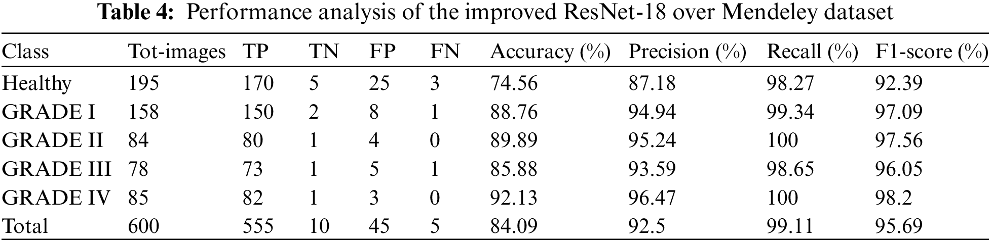
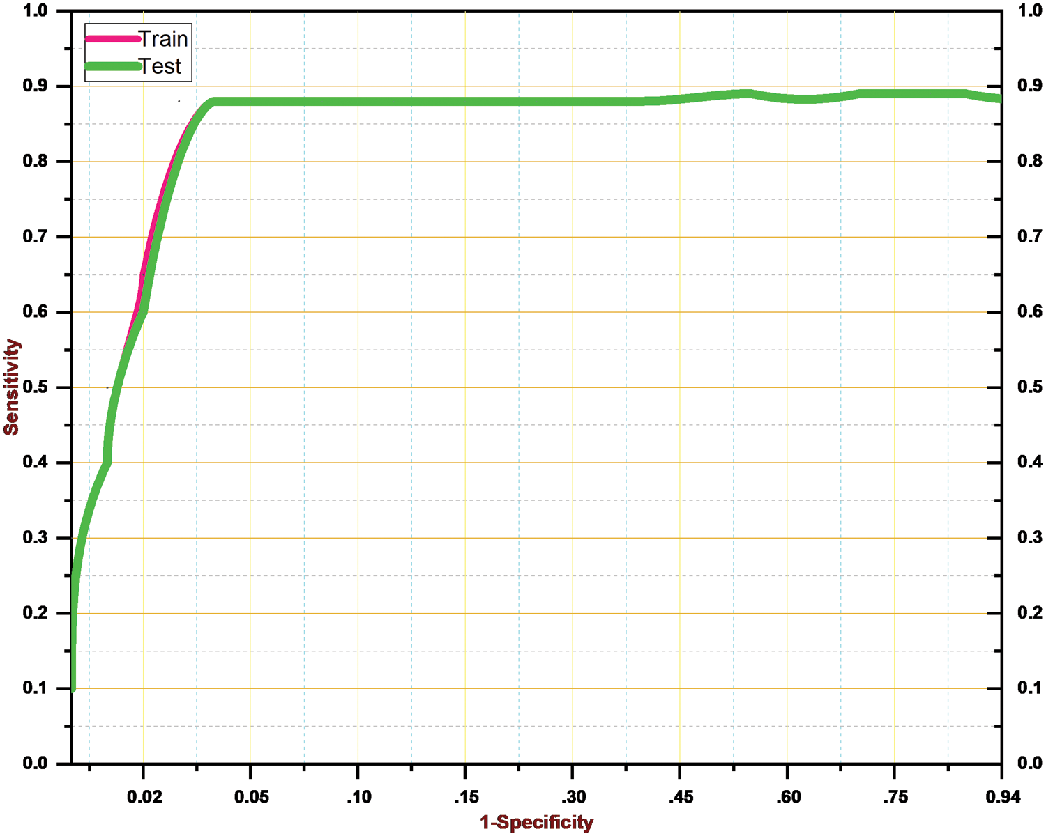
Figure 9: ROC curve for the proposed system

4.3 Performance Comparison of Improved ResNet-18 with Original ResNet-18

Here, we conduct an experiment using the Mendeley dataset to evaluate how well the suggested model performed as compared to the initial ResNet-18. We split the data similarly to train and test the baseline ResNet-18, using 70% (1400) images for training and 60% (600) images for testing the knee.

It is estimated that 553 out of 600 pics have been accurately classified. More specifically, because the Grade-I knee joint has characteristics comparable to those in the Healthy picture, three images for Grade I have been classed as FN (Healthy), while three images for Grade II have been classified as FP (Grade III). Furthermore, Grade III and Grade IV had the smallest gaps between knee joints, as evidenced by the classification of 10 Grade III knee images as FN (Healthy) and 5 Grade IV images as FP (Grade III), respectively. Additionally, 15 photos of healthy knees have been graded as Grade I. Results for the original ResNet-18 over the Mendeley Dataset are shown in Table 5. Fig. 10 displays the efficiency chart of the proposed model over the Mendeley dataset.

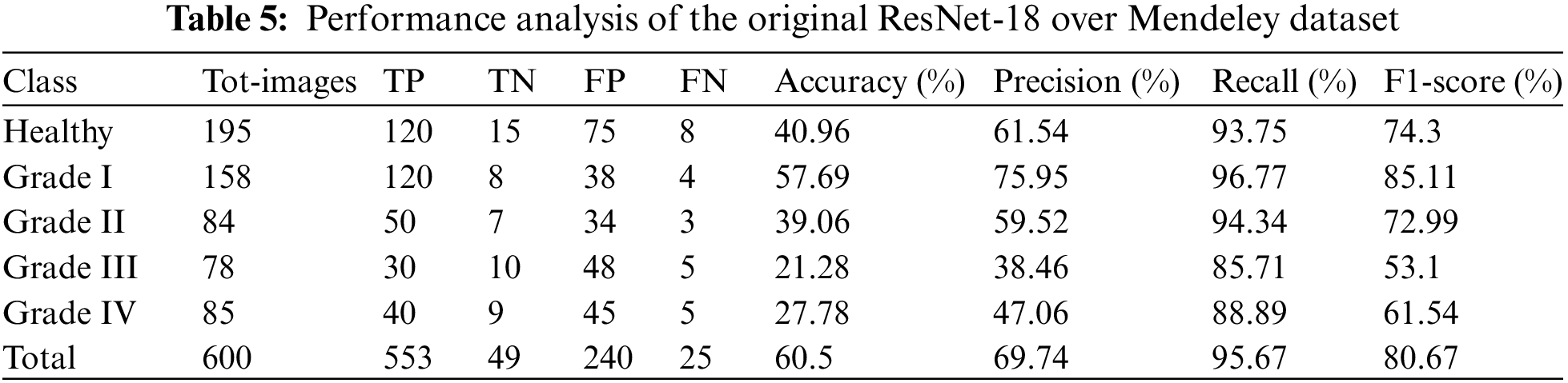
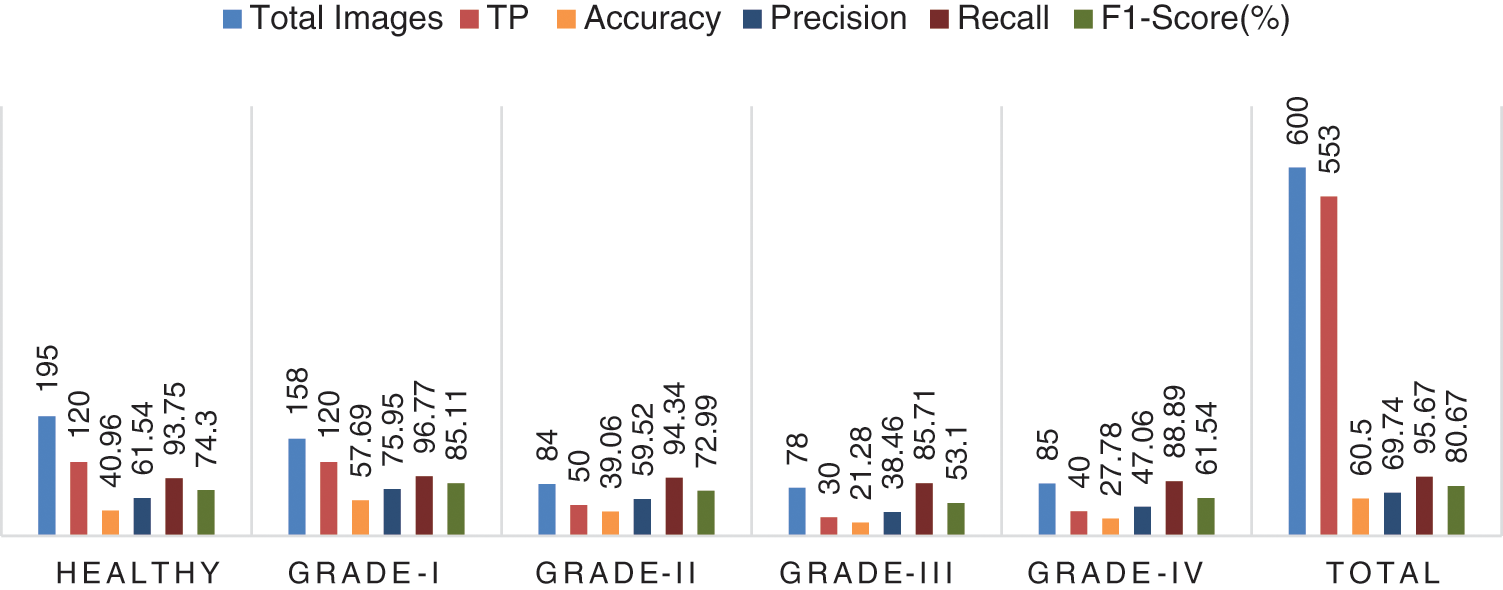
Figure 10: Performance plot of the proposed model over Mendeley test set

Furthermore, Fig. 11 shows a comprehensive confusion matrix for the multi-classification task carried out by our suggested model, the Enhanced ResNet-18. It can be shown that out of 600 photos, 555 have been correctly classified using our proposed approach, i.e., 150, 80, 73, 82, and 170 for Grade-I, Grade-II, Grade-IV, and Healthy classes, respectively. In Grade-I, 0 photos were identified as FN (Healthy), whereas in Grade II, only 4 pictures were classified as FP. This is becauseGrade-I knee joints share common characteristics with Healthy images (Grade-III). Moreover, Grade-III and Grade-IV had the smallest gaps between knee joints, with Grade-III having three knee images classed as FN (Healthy) and Grade-IV having only one image classified as FP (Grade-III). Additional Grade-I classifications include 5 photos of healthy knees. Our proposed approach has accuracy rates for Grade-I, Grade-II, Grade-III, Grade-IV, and Healthy classes of 88.76%, 89.89%, 85.88%, 92.13%, and 74.56% respectively.

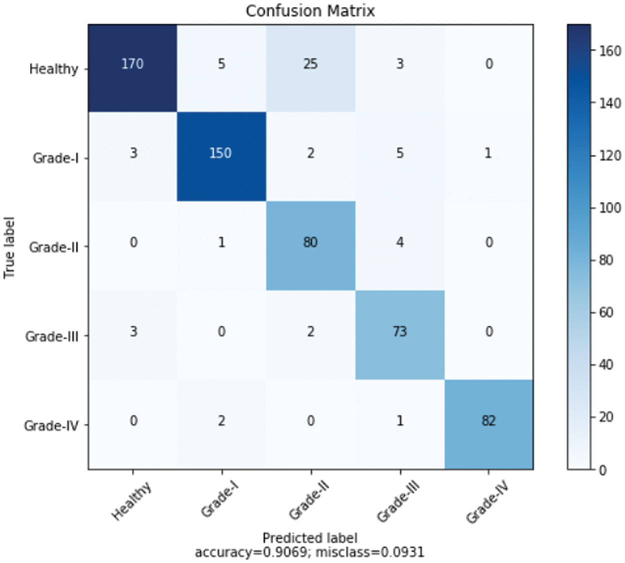
Figure 11: Confusion matrix for the proposed model over Mendeley dataset

4.4 Comparison with the Existing DL Models

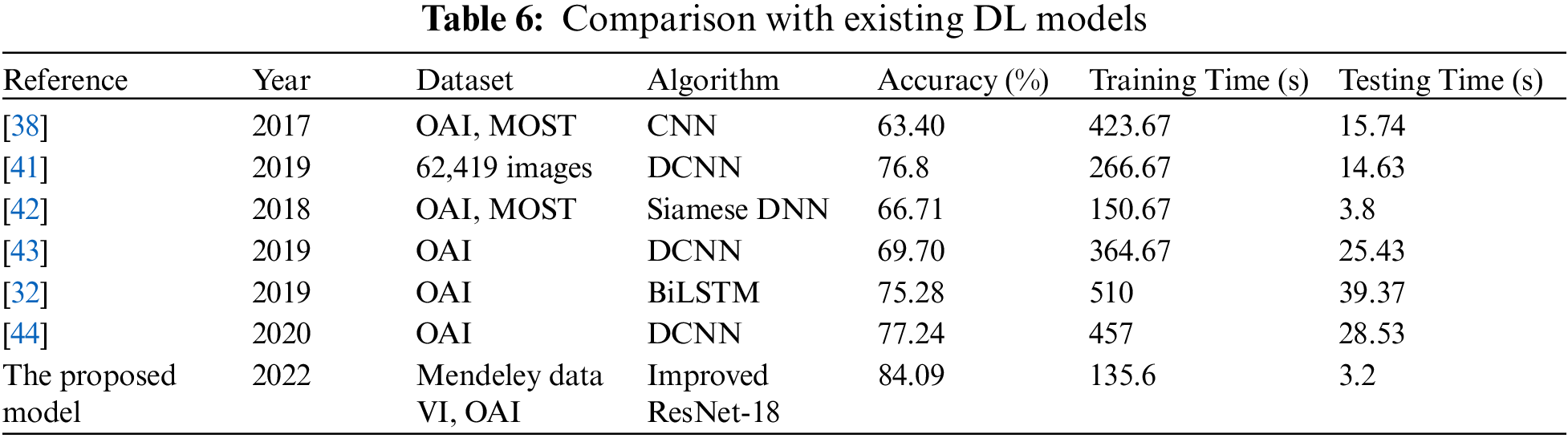
Here, we go over the deep learning models that are currently available for the diagnosis and classification of KOA illness. For the experimental evaluation, the majority of the Techniques used the OAI database. In [19], researchers utilized two separate sets of databases OAI and MOST, and implemented CNN to evaluate knee pictures. The algorithm’s testing time was 15.74 s, while the training time was 423.67 s. For the categorization, they were accurate to within 63.40 percent. In [34], 62,419 photos from the Institutes in South Korea were used to train the Deep CNN model for KOA recognition. With training and testing taking 266.67 and 14.63 s respectively, they were able to reach 76.8% accuracy. Siamese Deep NN was used by the authors in [35] to analyze OAI, MOST, and other datasets. They only achieved a meager 66.71 percent accuracy. 3.8 s were used for testing after 150.67 s were spent on training. Even though the testing and training timeframes are less than for the aforementioned procedures, the findings are still inaccurate. The OAI dataset was additionally used for the experiments in [36,37]. They were accurate at 69.70%, 75.28%, and 77.24% of the time, respectively The training and testing time was 364.67, and 25.43 s for [38] 510, and 39.37 s for [39], and 457, and 28.53 s for the [40]. Furthermore, our proposed algorithm has employed the Mendeley dataset for training and testing, and the OAI dataset for cross-validation.

For the Mendeley test set, it achieved 84.09 percent accuracy, and for the OAI dataset, 83.71 percent accuracy. Additionally, the experiments required less time than existing DL models because the training duration was 135.6 s, and the testing time was 2.9 s. Due to its dense construction, our suggested approach is reliable and effectively extracts information. Table 6 demonstrates that, in terms of accuracy, robustness, and training and testing times, our suggested technique performs better than all already used methods.

4.5 Cross-Validations

Using the OAI database, we perform a practical demo in this part to test the robustness of our suggested method. It includes 3 T MRI scans and knee joint X-rays that are graded using KL grading systems. The data were provided by 4,796 individuals, both male and female individuals aged up to 80. Patients who have undergone knee replacement surgery were also excluded from the database. Of the 4,796 individuals, 896 had healthy knees, and 3,900 had images from grades healthy, I, II, III, and IV respectively.

In addition, we tested our suggested model on 2500 photos, 500 of which were from each class, including grades health, I, II, III, and IV. More specifically, 50 photos of healthy knees out of 500 total photographs, 500 of which were graded as Grade-I, were wrongly classified. Due to minute discrepancies between Grade-I and Healthy pictures, 10 photos were wrongly labeled as showing healthy knees. Similar to this, 445, 420, and 430 of 500 Grade II, III, and IV knee radiographs in turn have been correctly categorized. Therefore, the suggested technique successfully divides the knee photos into five said categories. The grade-wise accuracy scores are 81.82%, 83.49%, 80.18%, 72.41%, and 75.44%, respectively. Our suggested Resnet-18 method outperforms the existing ResNet-18 in terms of results as shown in Table 7. The performance plot over cross-validation is shown in Fig. 12.

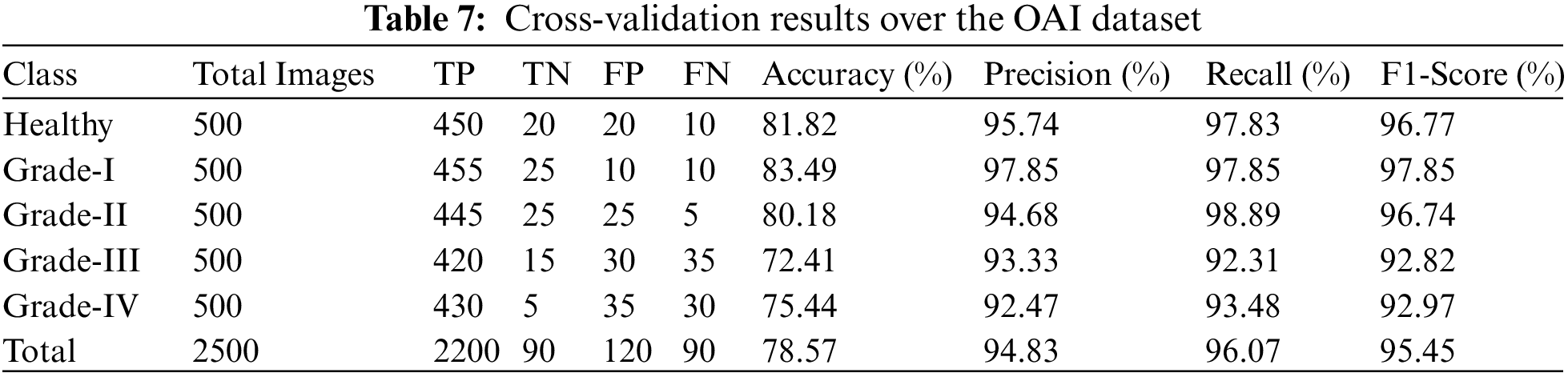
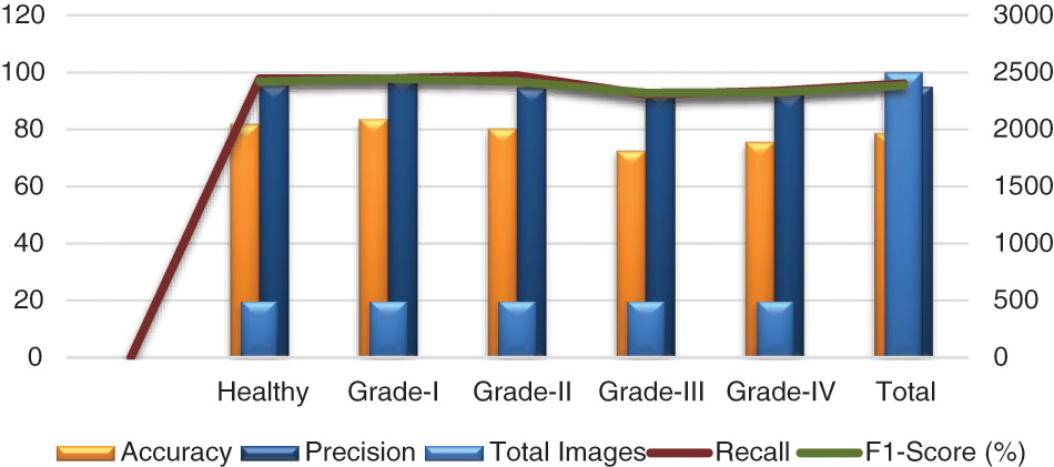
Figure 12: Performance plot of cross-validation over the OAI dataset

5  Conclusion

In this paper, we present a unique and simple deep learning-based model i.e., ResNet-18 for features extraction from segmented images and BiLSTM to identify KOA severity levels based on KL scoring, i.e., healthy and Grades: I, II, III, and IV respectively. Additionally, the offered system is built on an effective ResNet-18 pre-trained architecture that successfully addresses the issue of class imbalance in the dataset. In the research project, we employed two databases: the first dataset is Mendeley for training and testing, and the second dataset is OAI for cross-validation. To evaluate the effectiveness, numerous investigations have been carried out of the suggested framework attaining detection and recognition accuracy of 84.09%. More specifically, accuracy rates for the five grades/categories utilizing the Mendeley dataset were 74.56%, 88.76%, 89.89%, 85.88%, and 92.13%. The most crucial element of our study is to use it to identify the KOA quickly and accurately following the KL grading system while reducing the time and cost required for additional examination procedures. Due to the proposed pre-trained network’s short training and testing set require, the model effectively detects illnesses in knee images.

Although, we have proposed a system that is easy to use and train, however, we still want to improve the KOA detection accuracy. Therefore, in the future, we plan to use auto-fine-tuning techniques to enhance our suggested system in terms of accuracy. We will also use this technique in another area, including the identification of plant infections.

Acknowledgement: The researchers would like to thank the Deanship of Scientific Research, Qassim University for funding the publication of this project.

Funding Statement: The researchers would like to thank the Deanship of Scientific Research, Qassim University for funding the publication of this project.

Conflicts of Interest: The authors declare that they have no conflicts of interest to report regarding the present study.

References

1. P. S. Q. Yeoh, K. W. Lai, S. L. Goh, K. Hasikin et al., “Emergence of deep learning in knee osteoarthritis diagnosis,” Computational Intelligence and Neuroscience, vol. 2021, pp. 1–20, 2021. [Google Scholar]

2. Y. Du, R. Almajalid, J. Shan and M. Zhang, “A novel method to predict knee osteoarthritis progression on MRI using machine learning methods,” IEEE Transactions on Nanobioscience, vol. 17, no. 3, pp. 228–236, 2018. [Google Scholar] [PubMed]

3. K. A. Thomas, Ł. Kidziński, E. Halilaj, S. L. Fleming, G. R. Venkataraman et al., “Automated classification of radiographic knee osteoarthritis severity using deep neural networks,” Radiology: Artificial Intelligence, vol. 2, no. 2, pp. e190065, 2020. [Google Scholar] [PubMed]

4. A. Jamshidi, J. -P. Pelletier and J. Martel-Pelletier, “Machine-learning-based patient-specific prediction models for knee osteoarthritis,” Nature Reviews Rheumatology, vol. 15, no. 1, pp. 49–60, 2019. [Google Scholar] [PubMed]

5. K. Leung, B. Zhang, J. Tan, Y. Shen, K. J. Geras et al., “Prediction of total knee replacement and diagnosis of osteoarthritis by using deep learning on knee radiographs: Data from the osteoarthritis initiative,” Radiology, vol. 296, no. 3, pp. 584–593, 2020. [Google Scholar] [PubMed]

6. A. Jamshidi, M. Leclercq, A. Labbe, J. -P. Pelletier, F. Abram et al., “Identification of the most important features of knee osteoarthritis structural progressors using machine learning methods,” Therapeutic Advances in Musculoskeletal Disease, vol. 12, pp. 1759720X20933468, 2020. [Google Scholar] [PubMed]

7. M. Hochberg, K. Favors and J. Sorkin, “Quality of life and radiographic severity of knee osteoarthritis predict total knee arthroplasty: Data from the osteoarthritis initiative,” Osteoarthritis and Cartilage, vol. 21, pp. S11, 2013. [Google Scholar]

8. D. Giveki, H. Rastegar and M. Karami, “A new neural network classifier based on Atanassov’s intuitionistic fuzzy set theory,” Optical Memory and Neural Networks, vol. 27, no. 3, pp. 170–182, 2018. [Google Scholar]

9. R. Mahum, S. U. Rehman, O. D. Okon, A. Alabrah, T. Meraj et al., “A novel hybrid approach based on deep CNN to detect glaucoma using fundus imaging,” Electronics, vol. 11, no. 1, pp. 26, 2021. [Google Scholar]

10. D. Giveki and H. Rastegar, “Designing a new radial basis function neural network by harmony search for diabetes diagnosis,” Optical Memory and Neural Networks, vol. 28, no. 4, pp. 321–331, 2019. [Google Scholar]

11. R. Mahum, S. U. Rehman, T. Meraj, H. T. Rauf, A. Irtaza et al., “A novel hybrid approach based on deep cnn features to detect knee osteoarthritis,” Sensors, vol. 21, no. 18, pp. 6189, 2021. [Google Scholar] [PubMed]

12. W. Zhang, D. F. McWilliams, S. L. Ingham, S. A. Doherty, S. Muthuri et al., “Nottingham knee osteoarthritis risk prediction models,” Annals of the Rheumatic Diseases, vol. 70, no. 9, pp. 1599–1604, 2011. [Google Scholar] [PubMed]

13. N. Mijatovic, R. Haber, A. O. Smith and A. M. Peter, “A majorization-minimization algorithm for estimating the regularized wavelet-based density-difference,” in Int. Conf. on Computational Science and Computational Intelligence (CSCI), Las Vegas, NV, USA, IEEE, pp. 368–373, 2018. [Google Scholar]

14. X. Bu, J. Peng, C. Wang, C. Yu and G. Cao, “Learning an efficient network for large-scale hierarchical object detection with data imbalance: 3rd place solution to open images challenge 2019,” in arXiv preprint arXiv:1910.12044, 2019. [Google Scholar]

15. Y. Guo, Y. Liu, E. M. Bakker, Y. Guo and M. S. Lew, “CNN-RNN: A large-scale hierarchical image classification framework,” Multimedia Tools and Applications, vol. 77, no. 8, pp. 10251–10271, 2018. [Google Scholar]

16. D. Singh, V. Kumar and M. Kaur, “Densely connected convolutional networks-based COVID-19 screening model,” Applied Intelligence, vol. 51, no. 5, pp. 3044–3051, 2021. [Google Scholar] [PubMed]

17. N. Bien, P. Rajpurkar, R. L. Ball, J. Irvin, A. Park et al., “Deep-learning-assisted diagnosis for knee magnetic resonance imaging: Development and retrospective validation of MRNet,” PLoS Medicine, vol. 15, no. 11, pp. e1002699, 2018. [Google Scholar] [PubMed]

18. S. Kubkaddi and K. Ravikumar, “Early detection of knee osteoarthritis using SVM classifier,” IJSEAT, vol. 5, no. 3, pp. 259–262, 2017. [Google Scholar]

19. H. Faisal and R. Mahum, “Deep learning system for detecting the diabetic retinopathy,” in 2022 Mohammad Ali Jinnah University Int. Conf. on Computing (MAJICC), Karachi, Pakistan, IEEE, pp. 1–7, 2022. [Google Scholar]

20. A. E. Nelson, F. Fang, L. Arbeeva, R. J. Cleveland, T. A. Schwartz et al., “A machine learning approach to knee osteoarthritis phenotyping: Data from the FNIH biomarkers consortium,” Osteoarthritis and Cartilage, vol. 27, no. 7, pp. 994–1001, 2019. [Google Scholar] [PubMed]

21. M. Y. T. Hau, D. K. Menon, R. J. N. Chan, K. Y. Chung, W. W. Chau et al., “Two-dimensional/three-dimensional EOS™ imaging is reliable and comparable to traditional X-ray imaging assessment of knee osteoarthritis aiding surgical management,” The Knee, vol. 27, no. 3, pp. 970–979, 2020. [Google Scholar] [PubMed]

22. C. M. Bishop and N. M. Nasrabadi, “Pattern recognition and machine learning,” in Kurt F. Wendt Library Springer, vol. 4, no. 4, pp. 738, New York, 2006. [Online]. Available: https://link.springer.com/book/9780387310732 [Google Scholar]

23. A. Khamparia, B. Pandey, F. Al-Turjman and P. Podder, “An intelligent IoMT enabled feature extraction method for early detection of knee arthritis,” Expert Systems, pp. e12784, 2021. https://doi.org/10.1111/exsy.12784 [Google Scholar] [CrossRef]

24. G. B. Huang, Q. Y. Zhu and C. K. Siew, “Extreme learning machine: Theory and applications,” Neurocomputing, vol. 70, no. 1–3, pp. 489–501, 2006. [Google Scholar]

25. N. A. Segal, M. C. Nevitt, K. D. Gross, J. Hietpas, N. A. Glass et al., “The multicenter osteoarthritis study: Opportunities for rehabilitation research,” PM&R, vol. 5, no. 8, pp. 647–654, 2013. [Online]. Available: https://most.ucsf.edu/ [Google Scholar]

26. P. Vincent, H. Larochelle, I. Lajoie, Y. Bengio, P. A. Manzagol et al., “Stacked denoising autoencoders: Learning useful representations in a deep network with a local denoising criterion,” Journal of Machine Learning Research, vol. 11, no. 12, pp. 3371–3408, 2010. [Google Scholar]

27. E. Fix and J. L. Hodges, “Discriminatory analysis. Nonparametric discrimination: Consistency properties,” in International Statistical Review/Revue International de Statistique, vol. 57, no. 3, pp. 238–247, 1989. [Google Scholar]

28. A. Tiulpin, S. Klein, S. Bierma-Zeinstra, J. Thevenot, E. Rahtu et al., “Multimodal machine learning-based knee osteoarthritis progression prediction from plain radiographs and clinical data,” Scientific Reports,vol. 9, no. 1, pp. 1–11, 2019. [Google Scholar]

29. J. Marques, H. K. Genant, M. Lillholm and E. B. Dam, “Diagnosis of osteoarthritis and prognosis of tibial cartilage loss by quantification of tibia trabecular bone from MRI,” Magnetic Resonance in Medicine, vol. 70, no. 2, pp. 568–575, 2013. [Google Scholar] [PubMed]

30. R. Mahum, H. Munir, Z. -U. -N. Mughal, M. Awais, F. Sher Khan et al., “A novel framework for potato leaf disease detection using an efficient deep learning model,” Human and Ecological Risk Assessment: An International Journal, vol. 29, no. 2, pp. 303–326, 2023. [Google Scholar]

31. R. Mahum and S. Aladhadh, “Skin lesion detection using hand-crafted and DL-based features fusion and LSTM,” Diagnostics 2022, vol. 12, pp. 2974, 2022. [Google Scholar]

32. R. T. Wahyuningrum, L. Anifah, I. K. E. Purnama and M. H. Purnomo, “A new approach to classify knee osteoarthritis severity from radiographic images based on CNN-LSTM method,” in 2019 IEEE 10th Int. Conf. on Awareness Science and Technology (iCAST), Morioka, Japan, IEEE, pp. 1–6, 2019. [Google Scholar]

33. K. He, X. Zhang, S. Ren and J. Sun, “Deep residual learning for image recognition,” in Proc. of the IEEE Conf. on Computer Vision and Pattern Recognition, Las Vegas, NV, USA, pp. 192–195, 2016. [Google Scholar]

34. N. Shibata, M. Tanito, K. Mitsuhashi, Y. Fujino, M. Matsuura et al., “Development of a deep residual learning algorithm to screen for glaucoma from fundus photography,” Scientific Reports, vol. 8, no. 1, pp. 1–9, 2018. [Google Scholar]

35. S. Manjunatha and B. Annappa, “Real-time big data analytics framework with data blending approach for multiple data sources in smart city applications,” Scalable Computing: Practice and Experience, vol. 21,no. 4, pp. 611–623, 2020. [Google Scholar]

36. J. -S. Tan, B. K. Beheshti, T. Binnie, P. Davey, J. Caneiro et al., “Human activity recognition for people with knee osteoarthritis-a proof-of-concept,” Sensors, vol. 21, no. 10, pp. 3381, 2021. [Google Scholar] [PubMed]

37. C. G. Peterfy, E. Schneider and M. Nevitt, “The osteoarthritis initiative: Report on the design rationale for the magnetic resonance imaging protocol for the knee,” Osteoarthritis and Cartilage, vol. 16, no. 12, pp. 1433–1441, 2008. [Online]. Available: https://nda.nih.gov/oai/ [Google Scholar] [PubMed]

38. J. Antony, K. McGuinness, K. Moran and N. E. O’Connor, “Automatic detection of knee joints and quantification of knee osteoarthritis severity using convolutional neural networks,” in Int. Conf. on Machine Learning and Data Mining in Pattern Recognition, New York, NY, USA, Springer, pp. 195–198, 2017. [Google Scholar]

39. M. Lim, A. Abdullah, N. Jhanjhi, M. K. Khan and M. Supramaniam, “Link prediction in time-evolving criminal network with deep reinforcement learning technique,” IEEE Access, vol. 7, pp. 184797–184807, 2019. [Google Scholar]

40. M. B. Short, M. R. D’orsogna, V. B. Pasour, G. E. Tita, P. J. Brantingham et al., “A statistical model of criminal behavior,” Mathematical Models and Methods in Applied Sciences, vol. 18, no. supp01, pp. 1249–1267, 2008. [Online]. Available: https://www.blsa.nih.gov/ [Google Scholar]

41. J. Lim, J. Kim and S. Cheon, “A deep neural network-based method for early detection of osteoarthritis using statistical data,” International Journal of Environmental Research and Public Health, vol. 16, no. 7, pp. 1281, 2019. [Google Scholar]

42. H. Meisheri, R. Saha, P. Sinha and L. Dey, “A deep learning approach to sentiment intensity scoring of English tweets,” in Proc. of the 8th Workshop on Computational Approaches to Subjectivity, Sentiment and Social Media Analysis, Copenhagen, Denmark, pp. 193–199, 2017. [Google Scholar]

43. P. Chen, L. Gao, X. Shi, K. Allen and L. Yang, “Fully automatic knee osteoarthritis severity grading using deep neural networks with a novel ordinal loss,” Computerized Medical Imaging and Graphics, vol. 75, pp. 84–92, 2019. [Google Scholar] [PubMed]

44. R. Tri Wahyuningrum, A. Yasid and G. Jacob Verkerke, “Deep neural networks for automatic classification of knee osteoarthritis severity based on X-ray images,” in The 8th Int. Conf. on Information Technology: IoT and Smart City, Xi'an, China, pp. 110–111, 2020. [Google Scholar]