
 Submit a Paper
 Propose a Special lssue
 Open Access
ARTICLE
An Efficient 3D CNN Framework with Attention Mechanisms for Alzheimer’s Disease Classification
1 Department of Electronics and Communication Engineering, College of Engineering, Trivandrum, 695016, India
2 Department of Computer Science and Engineering, College of Engineering Muttathara, Trivandrum, 695008, India
3 Department of Electronics and Communication, Rajeev Gandhi Institute of Technology, Kottayam, 686501, India
4 Department of Electronics and Communication Engineering, Government Engineering College, Wayanad, 670644, India
* Corresponding Author: Sivakumar Ramachandran. Email:
Computer Systems Science and Engineering 2023, 47(2), 2097-2118. https://doi.org/10.32604/csse.2023.039262
Received 18 January 2023; Accepted 25 April 2023; Issue published 28 July 2023
 View Full Text
 Download PDF
Abstract
Neurodegeneration is the gradual deterioration and eventual death of brain cells, leading to progressive loss of structure and function of neurons in the brain and nervous system. Neurodegenerative disorders, such as Alzheimer’s, Huntington’s, Parkinson’s, amyotrophic lateral sclerosis, multiple system atrophy, and multiple sclerosis, are characterized by progressive deterioration of brain function, resulting in symptoms such as memory impairment, movement difficulties, and cognitive decline. Early diagnosis of these conditions is crucial to slowing down cell degeneration and reducing the severity of the diseases. Magnetic resonance imaging (MRI) is widely used by neurologists for diagnosing brain abnormalities. The majority of the research in this field focuses on processing the 2D images extracted from the 3D MRI volumetric scans for disease diagnosis. This might result in losing the volumetric information obtained from the whole brain MRI. To address this problem, a novel 3D-CNN architecture with an attention mechanism is proposed to classify whole-brain MRI images for Alzheimer’s disease (AD) detection. The 3D-CNN model uses channel and spatial attention mechanisms to extract relevant features and improve accuracy in identifying brain dysfunctions by focusing on specific regions of the brain. The pipeline takes pre-processed MRI volumetric scans as input, and the 3D-CNN model leverages both channel and spatial attention mechanisms to extract precise feature representations of the input MRI volume for accurate classification. The present study utilizes the publicly available Alzheimer’s disease Neuroimaging Initiative (ADNI) dataset, which has three image classes: Mild Cognitive Impairment (MCI), Cognitive Normal (CN), and AD affected. The proposed approach achieves an overall accuracy of 79% when classifying three classes and an average accuracy of 87% when identifying AD and the other two classes. The findings reveal that 3D-CNN models with an attention mechanism exhibit significantly higher classification performance compared to other models, highlighting the potential of deep learning algorithms to aid in the early detection and prediction of AD.Keywords
Neurodegenerative disorders encompass a wide variety of ailments characterized by the progressive degeneration of neurons and connections within the nervous system that underpins motor, balance, strength, perceptual, and cognitive functions. Neurodegeneration occurs at various levels. The disease advances from its initial Cognitive Normal (CN) stage to seriously advanced stages over time. A stage of complete brain cell death is reached gradually. Since the changes are irreversible, they are considered to be incurable. Hence, early detection can delay the degeneration of the cells and reduce the severity of the disease.
Alzheimer’s disease (AD) is the most prevalent disorder in the neurodegenerative class of diseases. It refers to a broad range of symptoms and manifestations rather than a specific disease that causes memory loss or other cognitive impairments that interfere with daily life. The various neuro-cognitive domains are complex attention, learning and memory, executive function, perceptual-motor, language, and social cognition. In mild cognitive impairment (MCI) there is a modest cognitive decline in one or more cognitive domains compared to the healthy state of the patient, and it will not affect everyday activities. According to the World Alzheimer Report, one person contracts dementia every three seconds, with 60% of these people suffering from AD. The estimated annual growth in patients by 2050 is 152 million, and the cost of patient care will be 2 trillion per annum by 2030 [1].
An important biomarker for the progression of AD is brain atrophy. Atrophy starts even before the appearance of amnestic symptoms [2]. Reduction in brain volume is an indicator of AD, which is evident in MRI images. Brain volume shrinkage results from the accumulation of senile plaques and neurofibrillary tangles throughout the brain. Functional and structural changes are visible in the brain MRIs of AD patients. The three plane views of brain MRI scans of CN, patients with MCI, and AD are shown in Fig. 1 for illustration. In the coronal view, there is visible atrophy (shrinkage) of the hippocampus, which is a key memory-related brain structure. This atrophy can be seen in the coronal view of the brain image of AD patients as a narrowing of the hippocampal region. In MCI, the atrophy of the hippocampus is usually milder than in AD, but it can still be visible in the coronal view. On the sagittal view, the temporal lobes frequently show atrophy, which may be visualized as a shrinkage of the temporal lobe in patients who have AD, although in MCI instances, the atrophy is generally less severe. In cases with AD, a decrease in the size of the parietal lobe is visible in the axial view; however, in MCI patients, this loss is usually not as severe. As there is no known treatment for AD, diagnosing it in its early stages is essential as it could delay abnormal brain atrophy.
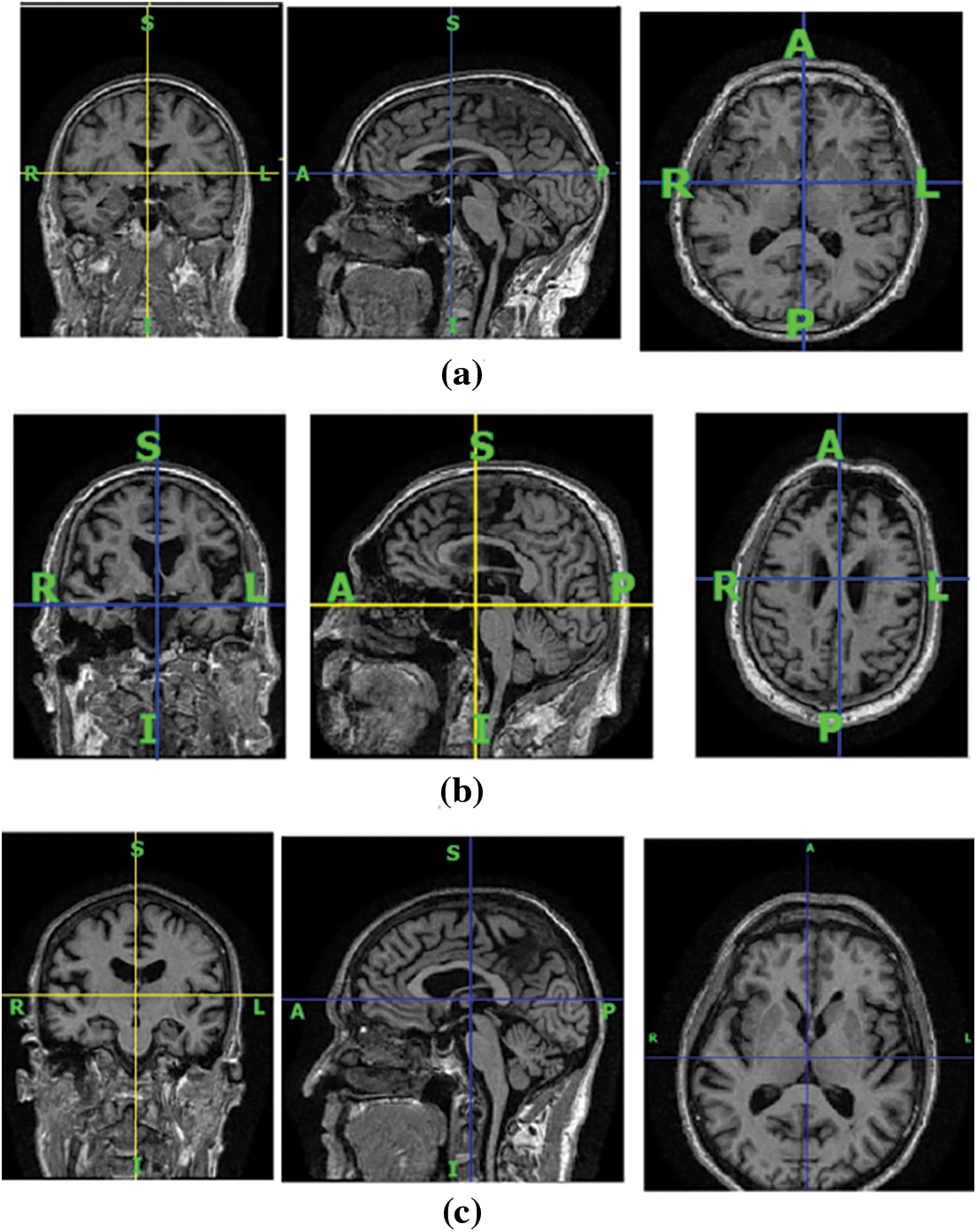
Figure 1: The brain MRI scans of human subjects in three different viewing planes. (a) Cognitive normal, (b) with AD, and (c) with MCI. The first column represents the coronal view, the second column represents the sagittal view, and the third column represents the axial view of the MRI scans of human subjects with and without brain disorders
Literature provides a substantial amount of research work on AD detection. Recent studies have demonstrated that deep learning techniques can classify AD more accurately than traditional image processing methods. The application of 2D CNNs in brain MRI images for AD diagnosis yields promising results. Major state-of-the-art studies convert 3D MRI scans to 2D image slices and apply 2D CNNs on those images for the classification of AD. Hence, features of the whole brain volume are not considered for analysis. In a 3D MRI scan, the relationship among 2D image slices is defined by their position in the three-dimensional space of the scanned object. Each 2D image slice represents a cross-sectional view of the object at a specific location along one of the three axes (x, y, or z). The images are acquired in correct order, typically along the z-axis, resulting in a stack of 2D image slices that together form a 3D volume. The spacing between the slices, known as the slice thickness, determines the distance between adjacent slices along the z-axis. By combining the information from all the 2D image slices, a 3D image of the object can be reconstructed, allowing for detailed visualization and analysis of the internal structure of the scanned object. The relationship among the 2D image slices is critical for the accurate interpretation of the 3D MRI scan and requires specialized software tools for image processing, analysis, and visualization. This research focuses on classifying AD using a novel 3D CNN framework.
3D CNNs are better suited to represent spatiotemporal information in comparison to 2D CNNs, which can only capture spatial information. In the field of computer vision, 3D CNNs can efficiently handle large volumes of data by learning both spatial and temporal features. 3D CNNs can process data in real-time, making them suitable for real-time applications. Moreover, they have been shown to generalize well to new data making them robust to variations in lighting, camera angle, and other factors that can affect the input quality.
Spatial and channel attention mechanisms are also added to the proposed pipeline to enhance the performance of the model. To the best of our knowledge, no study on AD classification using 3D CNN incorporates both spatial and channel attention mechanisms. The major contributions of this study are:
• A novel 3D CNN framework is designed for classifying AD, MCI, and CN.
• Channel and spatial attention mechanisms are incorporated with the 3D framework, which enhances the model performance.
• Three binary classifications: AD vs. CN, MCI vs. CN, AD vs. MCI, and a multi-class classification, AD vs. MCI vs. CN are performed and the results are compared.
The paper is structured as follows: Section 2 provides an overview of the current state-of-the-art methods for detecting Alzheimer’s disease in MRI images. In Section 3, the proposed approach for classifying normal and diseased images using 3D CNN and attention mechanisms is described. Section 4 contains information about the used data set for this study and the achieved results. A comparison with state-of-the-art techniques and a discussion of the results are also provided in this section. Section 5 concludes the paper by drawing conclusions.
The automatic detection of Alzheimer’s disease (AD) is still a hot topic of study in the scientific world. No research work has produced an outstanding result in AD prediction. Over the past decade, the research on detecting AD has become more dependent on deep learning (DL) techniques [3–5]. Gupta et al. [6] used cross-domain features to represent the MRI data. In that work, neuroimaging data is represented in natural image bases generated using a stacked autoencoder and then classified using convolution into three categories: AD, MCI, and healthy control. Brosch et al. [7] used deep belief networks (DBN) for learning features from complex three-dimensional brain images. DBNs are considered to be computationally expensive when applied to three-dimensional images due to a large number of trainable parameters. Liu et al. [8] used neuroimages acquired using different modalities to develop a sparse autoencoder-based algorithm that learns features from MRI images for image classification. This framework uses a zero-masking strategy for data fusion. Multiple deep 3D-CNN models are constructed in the study presented in [9] to learn the local features needed to predict AD in MRI images.
Li et al. [10] proposed a novel multipurpose DL framework for the classification of various levels of AD using MRI and PET images. The pipeline consists of various components, namely multi-task DL networks, principle component analysis, dropout, and stability selection. Shi et al. [11] proposed an efficient DL pipeline using multimodal stacked deep polynomial networks for AD detection using MRI and PET scan images. In [12], the problem of not having enough brain image data to train a network was fixed using pre-trained weights from large benchmark datasets of natural images. Using a novel 3D CNN approach, Yuan et al. [13] put forward a multi-center brain imaging classification framework for AD staging analysis. Multiple convolutional layers were used to extract gradient information in different directions, and spatial information at different scales was obtained through a summing operation. Ahmed et al. [14] employed a patch-based technique in conjunction with an ensemble of CNNs to learn MRI image features to differentiate healthy brains from diseased brains. In [15], 3D MRI volumes were converted into corresponding 2D image slices, and a pre-trained 2D CNN was used to classify image slices independently. Ebrahimi-Ghahnavieh et al. [16] proposed a ResNet-18 model utilizing transfer learning for AD detection. The framework uses the transfer of information from two-dimensional to three-dimensional image data. In [17], a deep ensemble learning framework using two sparse autoencoders was trained for feature learning to categorize normal and abnormal brain images. Venugopalan et al. [18] utilized deep learning techniques to analyze multimodal imaging data, namely MRI, genetic, and clinical test data for the classification of AD, MCI, and CN. MRI features are extracted using 3D-CNNs, while genetic and clinical data use stacked denoising auto-encoders for feature extraction. Zhang et al. in [19] presented a 3D residual self-attention network for AD classification. This network was able to capture local, global, and spatial features present in the MRI volume.
Prajapati et al. in [20] developed a dense neural network for the binary classification of AD and CN. To enhance the classifier’s accuracy, experiments were conducted using different activation functions and evaluated their results using 5-fold cross-validation. Orouskhani et al. [21] introduced a deep triplet network for brain MRI analysis and AD detection, using few-shot learning. To tackle the problem of over-fitting and poor performance due to the limited image samples, deep metric learning is employed in a deep triplet network with a conditional loss function, improving the accuracy of the model. A novel approach has been proposed to enhance the accuracy of diagnosing and classifying AD using a combination of MRI brain structural data and metabolite levels from the frontal and parietal regions [22]. The method utilizes a stacked auto-encoder neural network to classify individuals as either AD or healthy controls. 3D-CNN architecture composed of multiple convolutional layers, instance normalization, rectified linear units (ReLUs), and max-pooling layers were designed for classifying the cases of AD, MCI, and NC in [23].
A fair amount of research has also been reported on different methods of skull stripping, which is an important step in the pre-processing of raw MRI images. Existing works on skull stripping and the performance of different skull stripping (brain extraction) methods were surveyed in [24]. Schell et al. [25] introduced an artificial neural network-based algorithm for brain extraction called HD-BET that has undergone extensive validation. HD-BET outperforms commonly used brain extraction techniques. In the proposed work, this algorithm is used for brain extraction from raw MRI images.
The literature review shows that 2D-CNNs were used in a good amount of research for AD detection. The 2D image slices that are extracted from the 3D MRI data volume are used for classification. The main drawback of this approach is that 2D CNNs cannot figure out the relationship among 2D image slices in a 3D MRI scan. To fix this problem, a 3D CNN is deployed for detecting Alzheimer’s disease from MRI scans.
The proposed framework is comprised of two major stages: the pre-processing of raw MRI volume and the classification of pre-processed 3D data. During the pre-processing step, artifacts are removed, and the data is put into a standard format through a series of filtering steps. The pre-processed 3D MRI volume is then fed into a 3D CNN framework with attention mechanisms, which classifies the degeneration levels of Alzheimer’s disease. The proposed work used a mixed attention mechanism by combining channel and spatial attention [26] modules. Fig. 2 shows the schematic diagram of the proposed approach.
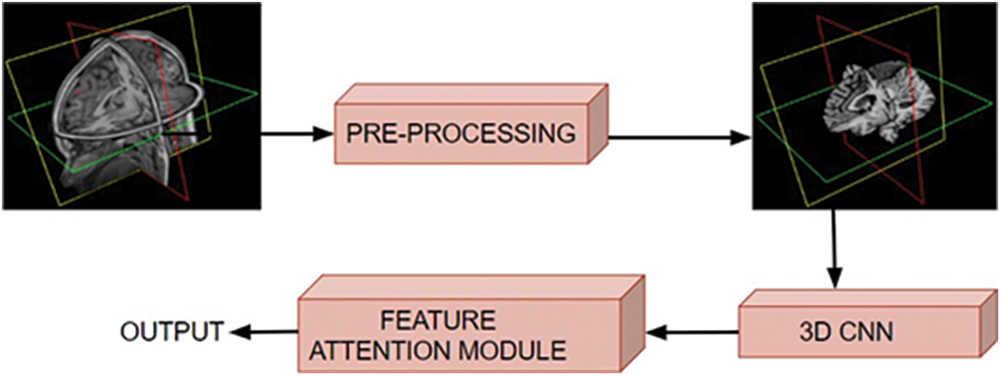
Figure 2: Schematic diagram of the proposed approach, where the input volumetric scans are pre-processed and fed to the 3D CNN for classifying various stages of brain dysfunction
The pre-processing of the raw images is the first step in every data-driven problem. The pre-processing stage consists of various operations, including noise removal, artifact removal, image enhancement, intensity normalization, skull stripping, image registration, and bias field correction. When dealing with raw MRI data, skull stripping is the most important step in the pre-processing stage. It takes out non-brain tissues such as the skull, dura, neck fat, and eyes from the brain MRI while keeping the brain tissues intact. The performance of the succeeding stages is greatly influenced by this process. The schematic diagram of the pre-processing stage is shown in Fig. 3.
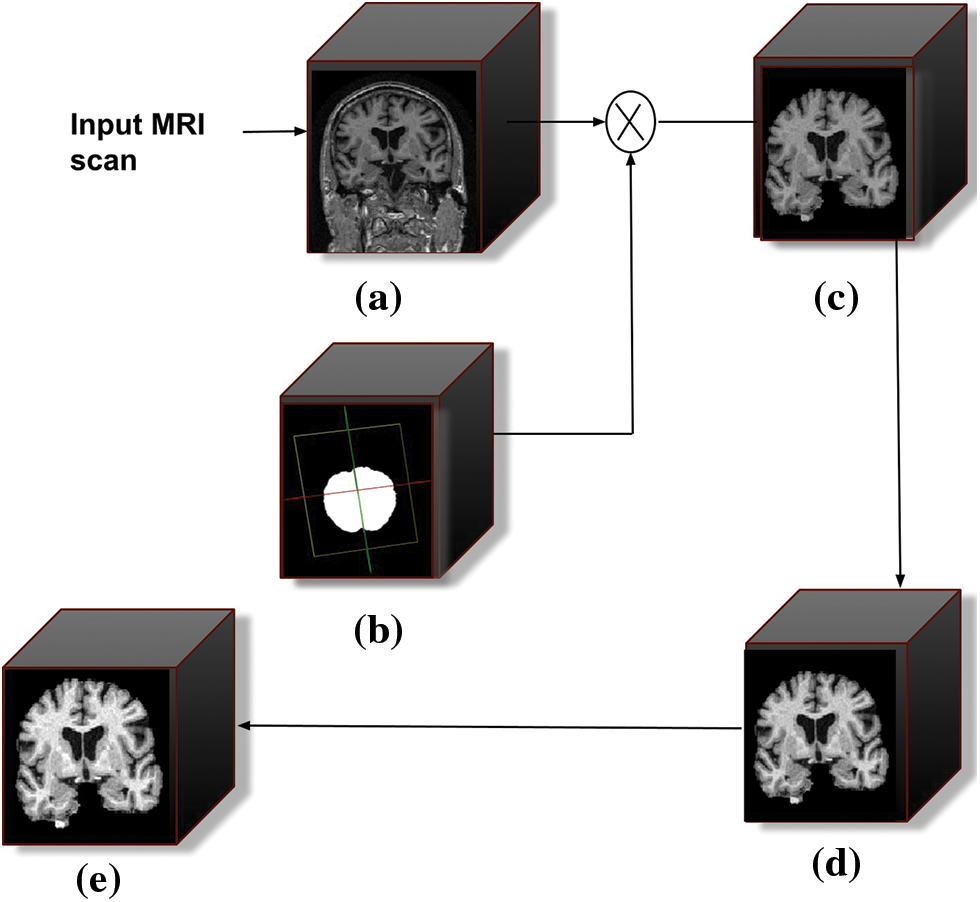
Figure 3: Schematic diagram of the pre-processing stages. (a) Filtered 3D input MRI scan, (b) represents the intermediate mask generated during skull stripping, (c) skull stripped output scan, (d) bias field corrected scan, and (e) represents intensity normalization scan
The images in the data set underwent various filtering procedures before the skull stripping. The data set contains scans obtained from the same person on the same day, which will result in redundant data that are essentially identical to one another. So these images are manually removed from the data set. The images included in the data set each have their unique image ID, subject ID, and the date of their acquisition. These data provide the basis for the filtering that is done manually. All the images are already pre-processed to some extent by the data set providers. The pre-processing of the scans was not consistent since each image was acquired at a different time stamp and with a different piece of imaging hardware. The unique image ID of each scan can be used to get a description of the pre-processing.
The primary filtering processes are followed by the removal of the tissues outside the meninges from the brain MRI volume. For brain extraction, many dedicated tools are publicly available. For this study, the skull stripping was done automatically using the HD-BET algorithm [25]. The algorithm generates the brain mask (Fig. 3b) for each input scan and is applied to the corresponding image.
Correction of the bias field is applied to the skull-stripped MRI scan. Due to the magnetic field variations, MR images exhibit image intensity non-uniformities. The imperfections in the field coils used in MRI systems and changes in magnetic susceptibility at the interfaces between anatomical tissue and air contribute to the intensity non-uniformities. The magnetic susceptibility varies slowly spatially, which is considered a signal gain change. This causes the white matter intensity to be the same as the grey matter intensity in some regions of the image. Tissue classifiers assume that the image intensities of tissues are uniform throughout the image, which is confounded by this problem. The present study used Brainsuite [27] for the bias field correction.
This software generates a sequence of local estimates of the signal gain alterations and based on this, the bias field corrector evaluates the region of the brain and estimates the corrected field.
In the next stage of pre-processing the bias field corrected MRI scans are intensity normalized for getting unit variance and zero mean. The mean intensity is subtracted from the input intensity and the result is divided by the standard deviation. The normalization process is defined as
where
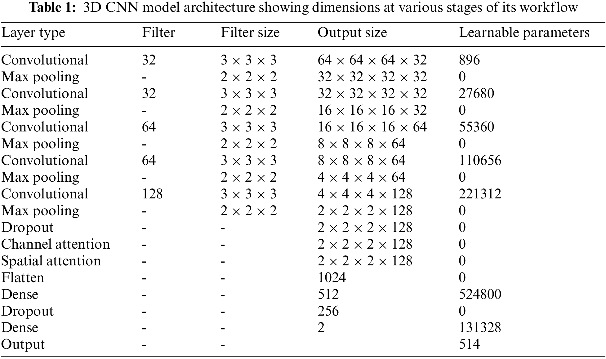
This work proposes a 3D CNN framework for identifying multiple classes that take the whole image volume as input and uses both spatial and channel attention mechanisms. The block schematic of the conceptual framework is shown in Fig. 4, which consists of two major building blocks, including the 3D convolution block and the attention (spatial and channel) block. The CNN framework used has five convolutional layers, five pooling layers, two fully connected layers, and a Softmax layer. The first two convolutional layers each include 32 filters, the subsequent two layers each contain 64 filters, and the final layer contains 128 filters. The 3D convolution applies a three-dimensional filter to capture low-level feature representation, which is computed by the movement of the filter in all three directions. Each filter is convolved with the whole volume of the input, which goes all the way to the full depth. The proposed model uses filters of size 3 × 3 × 3 in the convolutional layers. The output of each convolution produces a feature map assembled along the depth to constitute the output volume. There will be as many feature maps as there are filters.
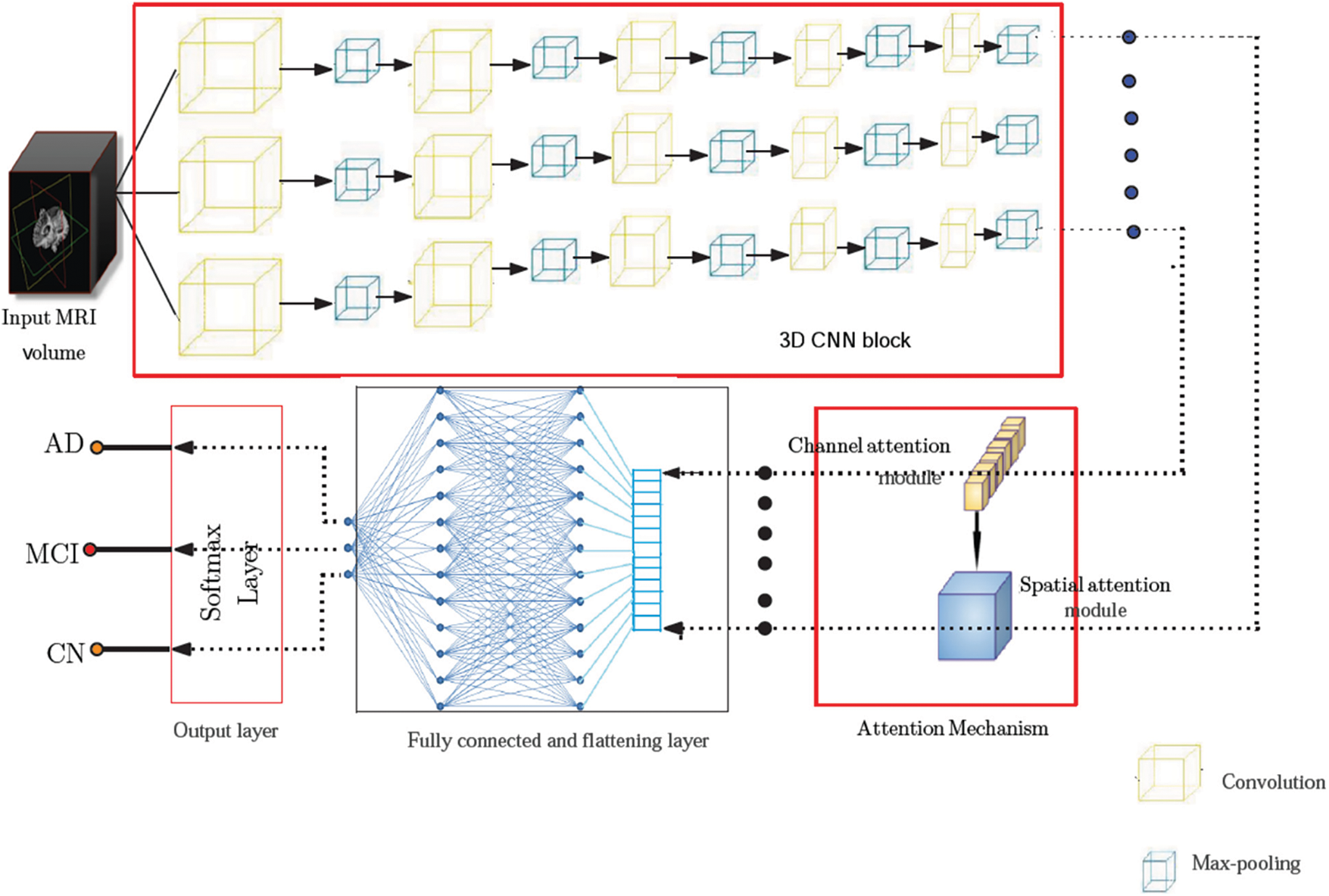
Figure 4: Model architecture showing various components of the proposed framework. The pre-processed input volume is fed to a 3D CNN framework comprising five convolutional layers, five pooling layers, two fully connected layers, and a Softmax layer. The feature map obtained from the 3D CNN is passed through an attention network consisting of spatial and channel attention mechanisms before it is fed to the final predicting stage
Each potential deep neural network architectural design shares the property that, as data moves into deeper layers through the system, the spatial dimension reduces. Dimensionality reduction is typically accomplished with max-pooling layers or by adjusting strides in convolutional layers. The architecture of the proposed system uses a stride of one and padding of one. A convolution operation with a stride size of one will produce output without losing much information. The reduced output size after the convolution operation will cause data loss, which is especially noticeable in the border voxels. To tackle this problem, zero padding is applied to the border voxels, which makes the analysis of the image easier. Zero padding and stride are set equal to one so that the output of each convolutional layer will have the same spatial size as the input volume. Rectified linear units (ReLU) are employed as activation functions and incorporated batch normalization into each convolutional layer. The computational complexity is reduced by incorporating a pooling operation that lowers the number of learnable parameters. The features located in a specific region of the feature map generated by a convolution layer are summarized by the pooling layer and are used for further processing. The study employs the max-pooling layers of dimension 2 × 2 × 2 voxel patches for dimensionality reduction. The flattening layer follows the 3D convolution block, which reduces the four-dimensional space to a single continuous linear vector. The output of the flattening layer is fed into a fully connected layer or dense layer. Our architecture uses two fully connected layers with 512 and 256 neurons, respectively. The output layer or Softmax layer is the final layer. The probabilities of the predicted classes are calculated using the Softmax activation function, and the class with the highest probability is considered to be the output. Table 1 provides the complete picture of the various components present in the proposed architecture.
Adam optimizer [28] is used to optimize the weights in the neural network layers for training the proposed network. The weights of the CNN layers were initialized using HeUniform initializers, which take samples from a uniform distribution. This initializer shows better performance when used along with the ReLU activation function [29].
The feature map obtained from the 3D CNN is passed through an attention network [26] to extract a more accurate feature representation of the input MRI volume. The intention behind the inclusion of the attention module is to select the top features from all the possible components of the input vector [30]. The attention mechanism is a key component in modern deep-learning models for image classification. It allows the model to selectively focus on relevant features and regions of the image, while ignoring irrelevant or noisy information. This is particularly important in medical imaging, where the images can be complex and contain many subtle details that are important for an accurate diagnosis. In a typical CNN, the same weight filters are applied to all regions of an input image, regardless of the content in each region. This means that the model may not pay enough attention to certain regions that are more relevant for a particular task. The attention mechanism solves this issue by allowing the model to focus dynamically on regions of the input image that are more relevant.
The proposed framework employs sequential channel and spatial attention modules, as shown in Fig. 5. This arrangement pays attention to both the channel and spatial dimensions separately, which improves the features of both dimensions. Thus the valuable features from both dimensions are enhanced. The feature maps obtained after the channel (
where, Ach and Asp represent the feature maps obtained after the channel and spatial attention modules, respectively, and
where, S is the sigmoid function
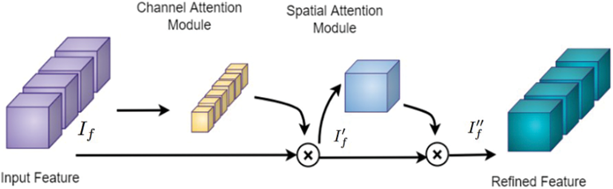
Figure 5: Attention block [26] consisting of channel and spatial attention modules, which are used to refine the feature map of the input MRI volume obtained from the 3D CNN
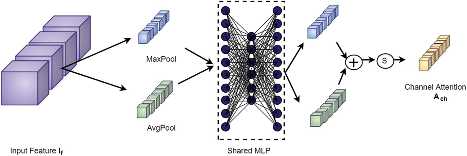
Figure 6: Channel attention block
The output from the channel attention module is then applied to the spatial attention module to investigate the inter-spatial relationship between the features. This attention mechanism concentrates on “where” the valuable information is positioned. Here, channel-wise average pooling and max-pooling are performed and combined to produce the feature descriptor. Then this descriptor is subjected to passing through a convolutional layer to obtain the spatial attention map as shown in Fig. 7. The spatial attention map
where, S, F, and [.] denote a sigmoid function, convolution operation with a fixed dimension filter, and concatenation operation of average pooled features and max-pooled features across the channel, respectively.
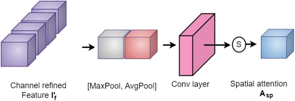
Figure 7: Spatial attention block
The MRI volumetric scans used for this study are obtained from Alzheimer’s Disease Neuroimaging Initiative (ADNI) data set [31]. The T1-weighted scans present in the data set are acquired using a 1.5 T MRI machine and comprised MRI scans from subjects with AD, MCI, and healthy cases. The ADNI data set comes with a metadata file that contains demographic information and pre-processing details for the included scans. The data providers have already applied various correction techniques to the scans to improve their quality. These techniques include Gradwarp, B1 non-uniformity correction, and N3 bias field correction.
One common issue with MRI scans is misinterpreted geometry due to problems with stochastic gradient descent. To address this issue and improve the accuracy of longitudinal behavior response, it is critical to correct for gradient non-linearity. This is accomplished using an automatic correction mechanism called Gradwarp [32]. Another issue that can affect the quality of MRI scans is contrast non-uniformities. B1 non-uniformity correction helps to address this problem by improving contrast uniformity across the image. Finally, N3 bias field correction is used to reduce low-frequency multiplicative noise in MRI images, which can otherwise obscure details and reduce image clarity.
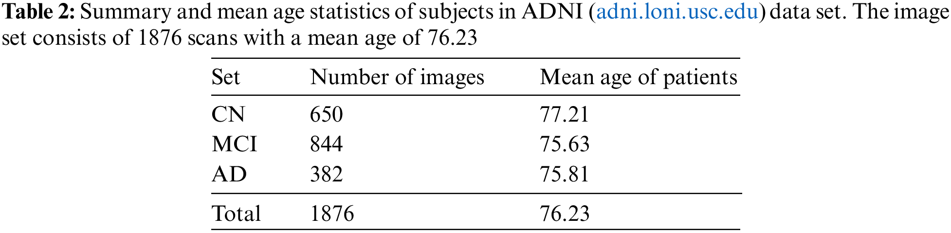
Overall, the pre-processing steps applied to the scans in the ADNI dataset aim to minimize common issues and improve the quality of the data for analysis and interpretation. A block schematic showing various pre-processing stages performed by data set providers is shown in Fig. 8. The readers can refer to [31] for more details regarding the data set. The pre-processed data serve as input for our proposed system and the details of the user data are summarized in Table 2.
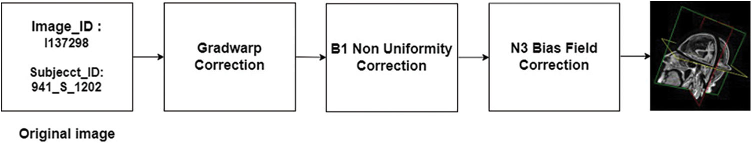
Figure 8: Stages of pre-processing introduced by ADNI. The MRI scans obtained from ADNI were pre-processed to a certain extent by the data set providers
The proposed model is evaluated based on Sensitivity (Se), Specificity (Sp), Precision (Pr), and F-measure (F) metrics which are defined as:
where TP, FP, TN, and FN denote the true positives, false positives, true negatives, and false negatives, respectively. Four classifications are carried out using the ADNI data set, namely NC vs. AD, MCI vs. CN, AD vs. MCI, and AD vs. MCI vs. CN. For the three binary classifications, a TP is counted when a scan labeled with the disease is correctly classified, and an FN when it is miss-classified. Also, TN is counted when an image of a healthy brain is perfectly predicted and FP when it is predicted as diseased. In the case of AD vs. CN classification TP is calculated concerning AD predictions and TN to CN predictions. Similarly, for the MCI vs. CN and AD vs. MCI classifications, TP is counted by considering the correct classification of MCI and AD, respectively, and TN is counted by considering the correct prediction of CN and MCI, respectively.
For the three-class classification (AD vs. MCI vs. CN), TP, TN, FP, and FN are calculated for each class. The evaluation metrics are computed for each class independently and then the unweighted mean is measured. In addition, the model performance of each binary classification is evaluated by plotting the receiver operating characteristic (ROC) curve and computing its underlying area, termed Area Under Curve (AUC). The overall performance of the proposed pipeline is also evaluated by assessing its accuracy, which is defined as:
For model training, the ADNI dataset is split into a train set containing 84% of the images and a test set with 16% of the remaining data. The train set is again subdivided into a train and validation set with 80% and 20% images, respectively. Since the data set has an imbalance in the number of scans for each class, data augmentation is carried out for the training data. The augmentation techniques employed include random rotation, noise addition, and flipping. The augmentation process increases the images of the AD, CN, and MCI classes by four, three, and two times, respectively. The batch size is set to 16 and the learning rate is empirically fixed at 0.001. The input brain MRI volumes of dimension 256 × 256 × 166 pixels are resized to 64 × 64 × 64 pixels, which serves as input to the proposed system.
The experiments are conducted using a GPU of NVIDIA-SMI 460.32.03 with CUDA Version 11.2, keeping Keras as the backend, on top of the Python 3.6 environment. Time complexity is approximately 2.1 GFlops. For training, the number of epochs is fixed at 100, and a dropout of 5% is incorporated to evade the problem of overfitting. Categorical cross-entropy loss function is used to adjust the network weights. During forward propagation, the generated output indicates confidence in the predicted labels, and these probabilities are compared with the true labels. During backpropagation partial derivative of the loss function is calculated corresponding to each network weight. Backpropagation iteratively adjusts the network weights to obtain a model with the least loss. Fig. 9 summarizes the learning curves of the model, showing both the loss (top) and accuracy (bottom) for the model on the train (blue) and validation (orange) data.
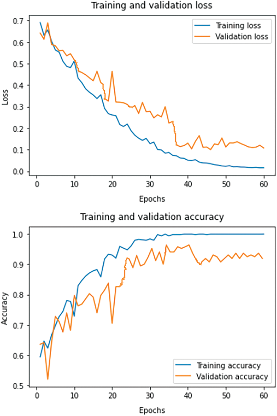
Figure 9: Loss and accuracy learning curves on the train and validation set for the proposed system
The results obtained for the proposed model employing 3D CNN are discussed in this section. The filtered image volumes obtained from the ADNI data set are again passed through various pre-processing stages, namely skull stripping, bias field correction, and intensity normalization. The two-dimensional view of the result after each pre-processing phase is shown in Fig. 10. The final 3D scan obtained after the various pre-processing stages is given as input to the proposed classification model.
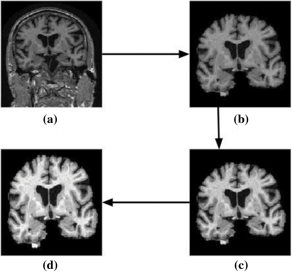
Figure 10: Two-dimensional view of the results obtained for various pre-processing stages using brain MRI scans as input. (a) Input image (b) skull stripped image (c) bias field corrected output, and (d) image obtained after intensity normalization
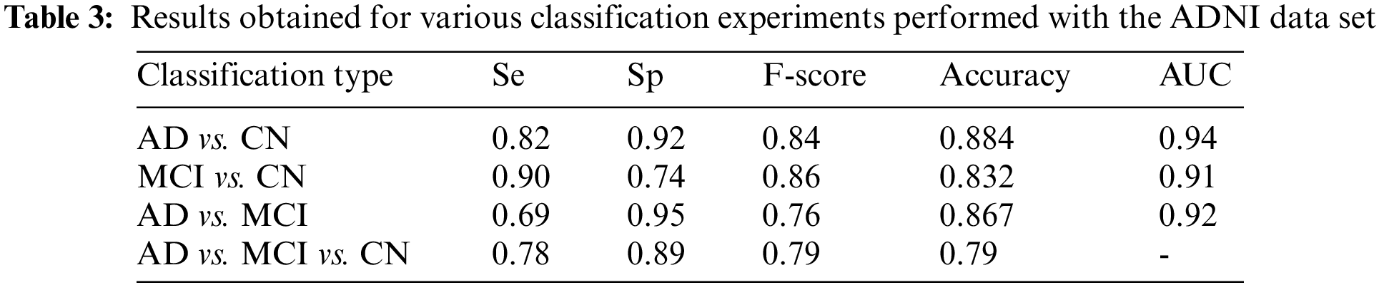
Four different classifications were carried out using the proposed model. The binary classification of AD vs. CN yielded an accuracy of 0.884 and a sensitivity of 0.82, corresponding to a maximum F1 score of 0.84. The AUC is obtained as 0.94. For a maximum F1 score of 0.86, an accuracy of 0.832 and a sensitivity of 0.90 were achieved for the MCI vs. CN classification. The AUC is obtained as 0.90 in this case. The accuracy and sensitivity achieved for the AD vs. MCI binary classification are 0.867 and 0.69, respectively, for a maximum F1 score of 0.76. The AUC is obtained as 0.92. For the three-class classification, AD vs. MCI vs. CN the accuracy obtained is 0.79, and the sensitivity and F1 score of the model are 0.78 and 0.79, respectively. The confusion matrix and ROC curves obtained are shown in Figs. 11 and 12 and the complete results of the experiments are summarized in Table 3.
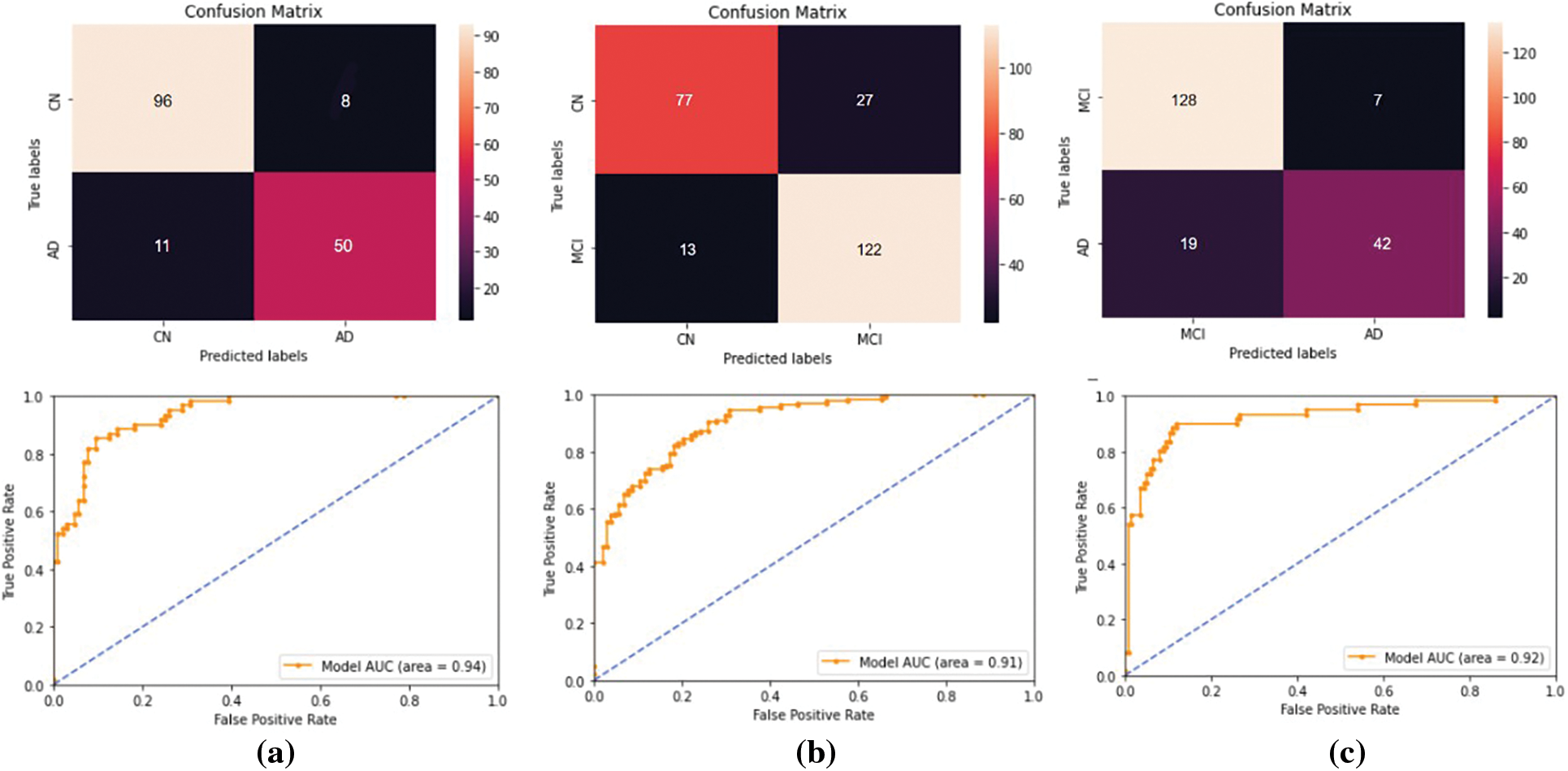
Figure 11: The performance metrics obtained for the binary classifications performed using the ADNI data set. For (a) AD vs. CN, (b) MCI vs. CN, and (c) AD vs. MCI classifications. The first row represents the confusion matrices and the second row represents the ROC curves
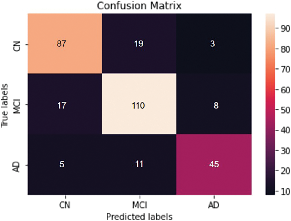
Figure 12: Confusion matrix obtained for the three classes- AD vs. MCI vs. CN classification
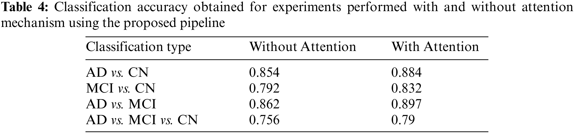
The results of the proposed model are examined and compared both with and without the integration of an attention mechanism. The accuracy obtained for AD vs. MCI classification is almost the same, and in all the other cases, the inclusion of an attention mechanism enhanced the proposed model performance. The observations obtained are depicted in Table 4.
In the past decade, there has been a surge in research projects focusing on machine learning and deep learning techniques. As a result, these methods have received increased attention in medical image processing and other research. The majority of CNN research to date has focused on 2D model construction and optimization, which are unquestionably crucial tasks for which they cannot interpret the relationship among 2D image slices in the 3D MRI scans. To address this challenge, a 3D CNN pipeline was developed that utilizes channel and spatial attention mechanisms to improve the classification results. The spatial and channel attention modules aggregate the most meaningful features that contribute to the respective classes of disease. Model performance shows a direct improvement with the addition of the attention module.
The results achieved using the proposed 3D CNN framework are compared with those obtained by state-of-the-art techniques that are currently available in the literature. Table 5 displays the comparison results obtained for the various methods that were considered. The proposed work uses segmented ROI volumetric scans, which are smaller in size, making classification computationally less expensive. The results obtained show that the three-class classification with attention is 4% more accurate than the classification without attention. As seen in Table 5, the research works that attempt to classify different stages of AD have ramped up, particularly in the last few years. The outcomes of these research works are inconsistent, even though they use a variety of ML and DL approaches. It has been found that the accuracy of the AD classification spans a broad range, from 58% [33] to 92% [34].
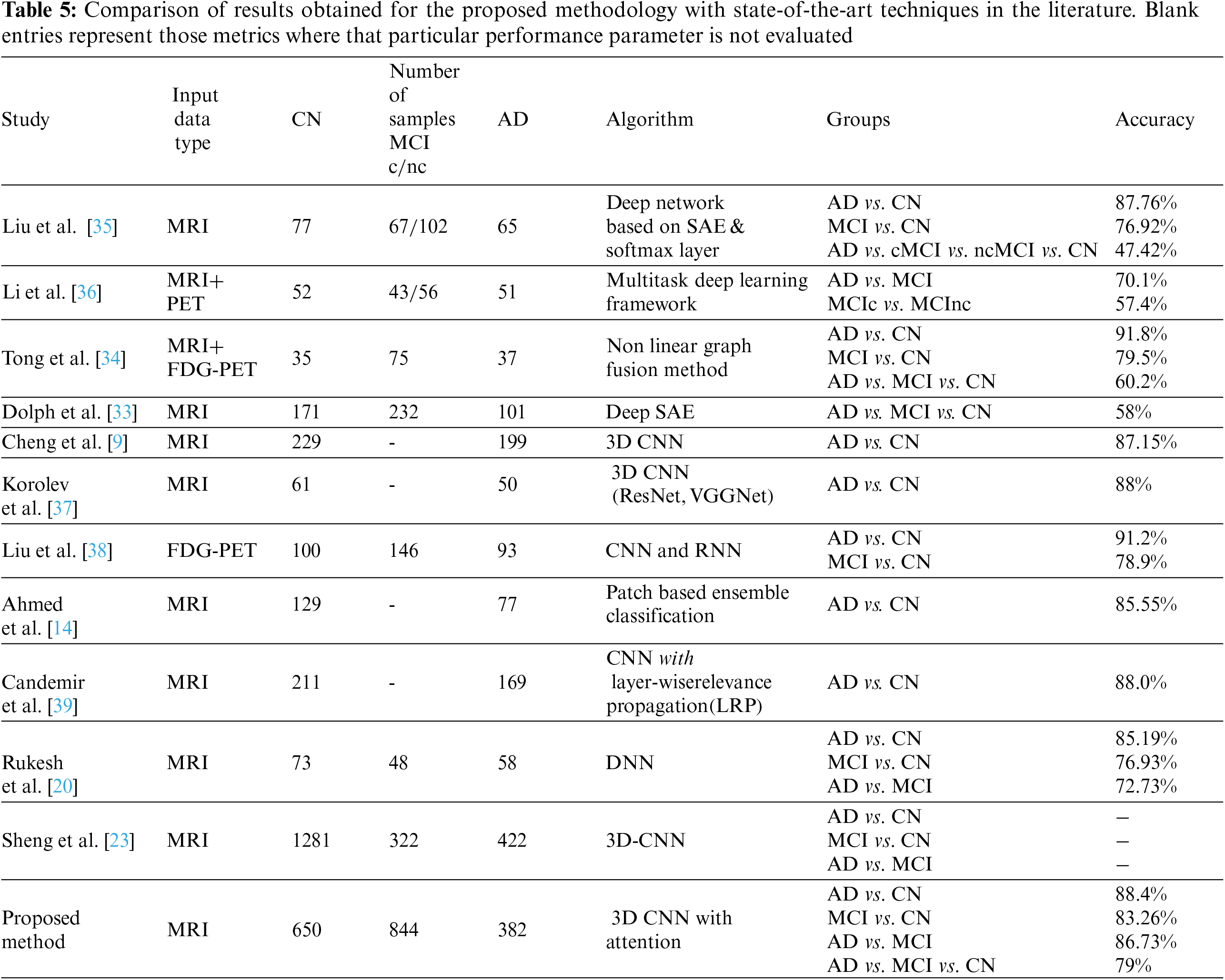
Compared to the results of other applications that use CNN, the accuracy of the AD classification has yet to reach its maximum value, which demonstrates the scope of this research topic. The results obtained using our proposed system are certainly not optimal for AD classification; nevertheless, when all of the experimented tasks are considered, our pipeline has its benefits.
Despite the major advances in MRI image processing, one of the most significant challenges researchers face today is the lack of standard annotated data sets for checking developed algorithms. Most of the research works published results with a limited amount of image data set [35,36]. A total of 1876 brain MRI scans obtained from the ADNI data set were used for training and validation in our study, which is a reasonable quantity compared to similar research works in the literature. The performance of deep learning models improves with an increased amount of data and helps network models to learn more representative and robust features of the underlying distribution, leading to improved performance. In addition to that, the proposed method of using 3D-CNN with attention mechanisms has contributed to performance improvement. Attention mechanisms are effective in improving the performance of deep learning models by allowing the model to focus on the most relevant features in the input data. Hence, it is not possible to definitively attribute the performance improvement to either the increase in data volume or the designed framework; both factors likely played a role in the improved performance of the proposed system.
The proposed CNN-based framework achieved an excellent area under the curve measures
The computerized analysis of brain MRI images for the automatic detection of certain pathologies, such as AD, MCI, and NC, among others, is of wide interest to the image processing and artificial intelligence research communities. The predictions made by deep learning methods are challenging to comprehend, even though they achieve high outcomes and often surpass the performance of human observers on a quantitative level. This makes it harder for such systems to be used in real diagnostic situations, where a detailed explanation of the decisions has to be provided. As black-box models, it is often hard to figure out why CNN fails or which image characteristics drive a particular network choice. This chasm might potentially be bridged with the use of novel visualization methods such as Layer-Wise Relevance Propagation [40,41] and deep Taylor decomposition [42]. To address this concern, our future work aims to build relevance maps for model assessment. These maps will highlight the areas of the brain that, according to CNN models, contributed the most to the decision-making process. In a clinical setting, the combination of CNN and relevance map unquestionably provides a potential technique for boosting the efficacy of CNN in categorizing MRIs of patients suspected of having Alzheimer’s disease (AD). Clinicians can compare classification results to understandable features provided in the relevance maps in clinically confusing scenarios, improving their ability to assess classification findings.
The proposed work involves the formulation and design of an efficient 3D CNN framework for the classification of Alzheimer’s disease using brain MRI data analysis. The proposed pipeline utilizes a mixed attention mechanism for enhancing the results. Our model provides a technique for dealing with 3D MRI scans by using a 3D convolutional neural network, in contrast to the majority of the research studies, which concentrate on 2D image slices extracted from volumetric scans. The proposed framework using channel attention could also be used for other medical image classification problems, as medical images are considered to have distinct responses across different channels. Even though the findings achieved are encouraging, deploying such a system would need substantial testing before it can be applied to real-life problems.
Funding Statement: The authors received no specific funding for this study.
Author Contributions: All authors have contributed equally to the study conception, design and manuscript preparation.
Availability of Data and Materials: The images used in this study are obtained from the publicly available ADNI data set (adni.loni.usc.edu). Informed consent was obtained for the data set providers from all individual participants included in the study.
Conflicts of Interest: The authors declare that they have no known competing financial interests or personal relationships that could have appeared to influence the work reported in this paper.
References
1. C. Patterson, World alzheimer report 2018, “Alzheimer’s disease international (ADI),” London, 2018. [Online]. Available: https://apo.org.au/sites/default/files/resource-files/2018-09/apo-nid260056.pdf [Google Scholar]
2. G. L. Wenk, “Neuropathologic changes in Alzheimer’s disease,” Journal of Clinical Psychiatry, vol. 64, no. 9, pp. 7–10, 2003. [Google Scholar] [PubMed]
3. T. Jo, K. Nho and A. J. Saykin, “Deep learning in Alzheimer’s disease: Diagnostic classification and prognostic prediction using neuroimaging data,” Frontiers in Aging Neuroscience, vol. 11, no. 220, 2019. [Google Scholar]
4. M. Tanveer, S. Richhariya, R. U. Khan, A. H. Rashid, P. Khanna et al., “Machine learning techniques for the diagnosis of Alzheimer’s disease: A review,” ACM Transactions on Multimedia Computing, Communications, and Applications (TOMM), vol. 16, no. 1s, pp. 1–35, 2020. [Google Scholar]
5. S. Leandrou, S. Petroudi, P. A. Kyriacou, C. C. Reyes-Aldasoro and C. S. Pattichis, “Quantitative mri brain studies in mild cognitive impairment and Alzheimer’s disease: A methodological review,” IEEE Reviews in Biomedical Engineering, vol. 11, 17955092, pp. 97–111, 2018. [Google Scholar] [PubMed]
6. A. Gupta, M. Ayhan, A. Maida, C. C. Reyes-Aldasoro and C. S. Pattichis., “Natural image bases to represent neuroimaging,” in Proc. 30th Int. Conf. on Machine Learning, Atlanta, Georgia, USA, pp. 987–994, 2013. [Google Scholar]
7. T. Brosch and R. Tam., “Manifold learning of brain mris by deep learning,” in Proc. Int. Conf. on Medical Image Computing and Computer-Assisted Intervention (MICCAI), Nagoya, Japan, pp. 633–640, 2013. [Google Scholar]
8. S. Liu, S. Liu, W. Cai, H. Che and S. Pujol, “Multimodal neuroimaging feature learning for multiclass diagnosis of Alzheimer’s disease,” IEEE Transactions on Biomedical Engineering, vol. 62, no. 4, pp. 1132–1140, 2014. [Google Scholar] [PubMed]
9. D. Cheng, M. Liu, J. Fu and Y. wang, “Classification of mr brain images by combination of multi-cnns for ad diagnosis,” in Proc. Ninth Int. Conf. on Digital Image Processing (ICDIP 2017), Hong Kong, China, pp. 875–879, 2017. [Google Scholar]
10. F. Li, L. Tran, K. H. Thung, S. Ji, D. Shen et al., “A robust deep model for improved classification of ad/mci patients,” IEEE Journal of Biomedical and Health Informatics, vol. 19, no. 5, pp. 1610–1616, 2015. [Google Scholar] [PubMed]
11. J. Shi, X. Zheng, Y. Li, Q. Zhang and S. Ying, “Multimodal neuroimaging feature learning with multimodal stacked deep polynomial networks for diagnosis of Alzheimer’s disease,” IEEE Journal of Biomedical and Health Informatics, vol. 22, no. 1, pp. 173–183, 2017. [Google Scholar] [PubMed]
12. M. Hon and N. M. Khan, “Towards Alzheimer’s disease classification through transfer learning,” in Proc. IEEE Int. Conf. on Bioinformatics and Biomedicine (BIBM), Kansas City, MO, USA, pp. 1166–1169, 2017. [Google Scholar]
13. L. Yuan, X. Wei, H. Shen, L. L. Zeng and D. Hu, “Multi-center brain imaging classification using a novel 3D CNN approach,” IEEE Access, vol. 6, pp. 49925–49934, 2018. [Google Scholar]
14. S. Ahmed, K. Y. Choi, J. J. Lee, B. C. Kim, G. R. Kwon et al., “Ensembles of patch-based classifiers for diagnosis of Alzheimer diseases,” IEEE Access, vol. 7, pp. 73373–73383, 2019. [Google Scholar]
15. A. Ebrahimi-Ghahnavieh, S. Luo and R. Chiong, “Transfer learning for Alzheimer’s disease detection on mri images,” in Proc. 2019 IEEE Int. Conf. on Industry 4.0, Artificial Intelligence, and Communications Technology (IAICT), Bali, Indonesia, pp. 133–138, 2019. [Google Scholar]
16. A. Ebrahimi-Ghahnavieh, S. Luo and R. Chiong, “Introducing transfer learning to 3d resnet-18 for Alzheimer’s disease detection on mri images,” in Proc. 2019 IEEE Int. Conf. on Image and Vision Computing New Zealand (IVCNZ), Wellington, New Zealand, pp. 1–6, 2020. [Google Scholar]
17. N. An, H. Ding, J. Yang, R. Au and T. F. Ang, “Deep ensemble learning for Alzheimer’s disease classification,” Journal of Biomedical Informatics, vol. 105, pp. 103411, 2020. [Google Scholar] [PubMed]
18. J. Venugopalan, L. Tong, H. R. Hassanzadeh and M. D. Wang, “Multimodal deep learning models for early detection of Alzheimer’s disease stage,” Scientific Reports, vol. 11, no. 1, pp. 1–13, 2021. [Google Scholar]
19. X. Zhang, L. Han, W. Zhu, L. Sun and D. Zhang, “An explainable 3d residual self-attention deep neural network for joint atrophy localization and Alzheimer’s disease diagnosis using structural mri,” IEEE Journal of Biomedical and Health Informatics, vol. 26, no. 11, pp. 5289–5297, 2021. [Google Scholar]
20. R. Prajapati, U. Khatri and G. R. Kwon, “An efficient deep neural network binary classifier for Alzheimer’s disease classification,” in Proc. 2021 IEEE Int. Conf. on Artificial Intelligence in Information and Communication (ICAIIC), Jeju Island, South Korea, pp. 231–234, 2021. [Google Scholar]
21. M. Orouskhani, S. Rostamian, F. S. Zadeh, M. Shafiei and Y. Orouskhani, “Alzheimer’s disease detection from structural mri using conditional deep triplet network,” Neuroscience Informatics, pp. 100066, 2022. [Google Scholar]
22. H. Wang, T. Feng, Z. Zhao, X. Bai, G. Han et al., “Classification of Alzheimer’s disease based on deep learning of brain structural and metabolic data,” Frontiers in Aging Neuroscience, vol. 681, 2022. [Google Scholar]
23. S. Liu, A. V. Masurkar, H. Rusinek, J. Chen, B. Zhang et al., “Generalizable deep learning model for early Alzheimer’s disease detection from structural mris,” Scientific Reports, vol. 12, no. 1, pp. 17106, 2022. [Google Scholar] [PubMed]
24. P. Kalavathi and V. Prasath, “Methods on skull stripping of mri head scan imagesa review,” Journal of Digital Imaging, vol. 29, no. 3, pp. 365–379, 2016. [Google Scholar] [PubMed]
25. M. Schell, I. Tursunova, I. Fabian, D. Bonekamp, U. Neuberger et al., “Automated brain extraction of multi-sequence mri using artificial neural networks,” in Proc. European Congress of Radiology- ECR 2019, Vienna, Austria, 2019. [Online]. Available: https://dx.doi.org/10.26044/ecr2019/C-2088 [Google Scholar] [CrossRef]
26. S. Woo, J. Park, J. Y. Lee and I. S. Kweon, “Cbam: Convolutional block attention module,” in Proc. of the European Conf. on Computer Vision (ECCV), Munich, Germany, pp. 3–19, 2018. [Google Scholar]
27. D. W. Shattuck and M. R. Leahy, “Brainsuite: An automated cortical surface identification tool,” Medical Image Analysis, vol. 29, no. 3, pp. 129–142, 2002. [Google Scholar]
28. D. P. Kingma and J. Ba, “Adam: A method for stochastic optimization,” arXiv preprint arXiv:1412.6980, 2014. [Google Scholar]
29. K. He, X. Zhang, S. Ren and J. Sun, “Delving deep into rectifiers: Surpassing human-level performance on imagenet classification,” in Proc. IEEE Int. Conf. on Computer Vision, Santiago, Chile, pp. 1026–1034, 2015. [Google Scholar]
30. D. Bahdanau, K. Cho and Y. Bengio, “Neural machine translation by jointly learning to align and translate, arXiv preprint arXiv:1409.0473, 2014. [Google Scholar]
31. R. C. Petersen, P. S. Aisen, L. A. Beckett, M. C. Donohue, A. C. Gamst et al., “Alzheimer’s disease neuroimaging initiative (ADNIClinical characterization,” Neurology, vol. 74, no. 3, pp. 201–209, 2010. [Google Scholar] [PubMed]
32. T. Torfeh, R. Hammound, M. McGarry, N. Al-Hammadi and G. Perkins, “Development and validation of a novel large field of view phantom and a software module for the quality assurance of geometric distortion in magnetic resonance imaging disease stage,” Magnetic Resonance Imaging, vol. 37, no. 7, pp. 939–949, 2015. [Google Scholar]
33. C. V. Dolph, M. Alam, Z. Shboul, M. D. Samad and K. M. Iftekharuddin, “Deep learning of texture and structural features for multiclass Alzheimer’s disease classification,” in Proc. IEEE Int. Joint Conf. on Neural Networks (IJCNN), Anchorage, AK, USA, pp. 2259–2266, 2017. [Google Scholar]
34. T. Tong, K. Gray, Q. Gao, L. Chen and D. Rueckert, “Nonlinear graph fusion for multi-modal classification of Alzheimer’s disease,” in Proc. Int. Workshop on Machine Learning in Medical Imaging, Munich, Germany, pp. 77–84, 2015. [Google Scholar]
35. S. Liu, S. Liu, W. Cai, S. Pujol, R. Kikinis et al., “Early diagnosis of Alzheimer’s disease with deep learning,” in Proc. IEEE 11th Int. Symp. on Biomedical Imaging (ISBI), Beijing, China, pp. 1015–1018, 2014. [Google Scholar]
36. F. Li, L. Tran, K. H. Thung, S. Ji, D. Shen et al., “Robust deep learning for improved classification of ad/mci patients,” in Proc. Int. Workshop on Machine Learning in Medical Imaging, Boston, USA, pp. 240–247, 2014. [Google Scholar]
37. S. Korolev, A. Safiullin, M. Belyaev and Y. Dodonova, “Residual and plain convolutional neu ral networks for 3d brain mri classification,” in Proc. IEEE 14th Int. Symp. on Biomedical Imaging (ISBI 2017), Melbourne, Australia, pp. 835–838, 2017. [Google Scholar]
38. M. Liu, D. Cheng, W. Yan and A. D. N. Initiative, “Classification of Alzheimer’s disease by combination of convolutional and recurrent neural networks using fdgpet images,” Frontiers in Neuroinformatics, vol. 12, pp. 35, 2018. [Google Scholar] [PubMed]
39. S. Candemir, X. V. Nguyen, L. M. Prevedello, M. T. Bigelow, R. D. White et al., “Predicting rate of cognitive decline at baseline using a deep neural network with multidata analysis,” Journal of Medical Imaging, vol. 7, no. 4, pp. 044501, 2020. [Google Scholar] [PubMed]
40. M. Böhle, F. Eitel, M. Weygandt and K. Ritter, “ “Layer-wise relevance propagation for explaining deep neural network decisions in mri-based Alzheimer’s disease classification,” Frontiers in Aging Neuroscience, vol. 11, pp. 194, 2019. [Google Scholar]
41. S. Bach, A. Binder, G. Montavon, F. Klauschen, K. R. Müller et al., “On pixel-wise explana tions for non-linear classifier decisions by layer-wise relevance propagation,” PLoS One, vol. 10, no. 7, pp. e0130140, 2015. [Google Scholar] [PubMed]
42. G. Montavon, W. Samek and K. R. Müller, “Methods for interpreting and understanding deep neural networks,” Digital Signal Processing, vol. 73, pp. 1–15, 2018. [Google Scholar]
Cite This Article
 Copyright © 2023 The Author(s). Published by Tech Science Press.
This work is licensed under a Creative Commons Attribution 4.0 International License , which permits unrestricted use, distribution, and reproduction in any medium, provided the original work is properly cited.
 Downloads
 Citation Tools