3D-CNNHSR: A 3-Dimensional Convolutional Neural Network for Hyperspectral Super-Resolution

1  Introduction

Hyperspectral remote sensing, an advanced method of remote sensing, has gained significant popularity over the past decade. This technique utilizes charge-coupled devices (CCDs) as a detector system to capture numerous spectral channels [1–3]. The signal of a pixel often represents the interaction of electromagnetic radiation from different constituents within the pixel. Hyperspectral images (HSI) sets are employed to spectrally identify and classify the same objects on the surface. Reflectance information of objects is collected through hyperspectral remote sensing, which consists of hundreds of contiguous and narrow bands spanning a specific electromagnetic spectrum. The HSI data cubes encompass both spatial and spectral content [1–3]. Therefore, HSI that is collected has a very high spectral resolution so that the discrimination between the objects can be done by their spectral signature. Because of spectral content, HSI is widely used in computer vision and remote sensing applications, such as change detection [4,5], geological exploration [6], and object detection [7]. Among the various applications of hyperspectral data analysis, agriculture is one of the most promising areas, where hyperspectral data be used to control all stages of the crop cycle, from soil preparation through sowing and growth to harvesting. Additionally, HSI can be utilized for crop illness, soil fertility, plant development, fruit ripeness, parasites, and other inspections in fields and plantations of all types.

As current imaging sensor technologies have limitations, there exists a trade-off between spatial and spectral resolution. Hyperspectral imaging (HSI) often suffers from low spatial resolution, which hampers its performance in various applications. Increasing the number of pixels per unit area can improve the spatial resolution of HSI, but it leads to a reduction in available light and critical degradation of image quality due to shot noise. Moreover, increasing chip size results in higher capacitance, slowing down the rate of charge transfer. Therefore, both approaches are not feasible. Signal post-processing techniques offer a solution to enhance the measured signal and overcome the low spatial resolution of HSIs. One such technique is super-resolution (SR) reconstruction, which utilizes one or more low-resolution (LR) images to obtain a high-resolution (HR) image. This approach is cost-effective and can make use of existing LR imaging systems. HSIs have significant practical utility, making it crucial to enhance their spatial resolution.

Various methods have been proposed to improve the spatial resolution of HSI using high-spatial-resolution sources [8]. Image fusion can be applied when an auxiliary image with high spatial resolution, such as a multispectral image, is available. Techniques like maximum a posteriori (MAP) estimation [8], stochastic mixing model-based methods, and others [9,10] have been proposed. However, dictionary-based fusion methods, including spectral dictionary and spatial dictionary-based methods, are predominant in hyperspectral and multispectral image fusion. Nevertheless, these methods do not effectively utilize spatial and spectral content.

Sub-pixel-based analysis aims to extract valuable information from pixels for various applications. Spectral Mixture Analysis (SMA) [11] is utilized to estimate the fractional abundance of pure ground objects within a pixel. The extraction and estimation of end members can be done separately or treated as a blind signal decomposition problem, for which techniques like convex optimization [12], non-negative matrix factorization [13,14], and neural network-based approaches are commonly employed [15]. Sub-pixel level-based target detection methods have also been proposed to identify objects of interest within a pixel [16,17]. Soft classification methods can address the challenges of classification in low-spatial-resolution hyperspectral images (HSI) [17]. The emergence of sub-pixel mapping (SPM) aims to generate a classification map by utilizing fractional abundance images to predict the locations of land cover classes within mixed pixels [18–20]. Numerous methods have been proposed, including those that employ structural similarity [21], pixel/sub-pixel spatial attraction model [22], pixel swapping algorithm [23], maximum a posteriori (MAP) [24,25] mode, Markov random field (MRF) [26,27], artificial neural network (ANN) [28–30], simulated annealing [31], total variant model [32], support vector regression [33], and collaborative representation [34]. However, it is important to note that these techniques only overcome spatial resolution limitations in specific applications.

While many previous approaches have focused on single-band or grayscale super-resolution under controlled conditions, they encounter challenges in real-world scenarios with a substantial number of bands. Single-image super-resolution (SR) aims to reconstruct high spatial resolution images from low spatial resolution images. Traditional linear interpolation techniques, such as bilinear and bicubic methods, are commonly employed, but they often introduce side effects like edge blurring, ringing, and jagged artifacts. Some studies [31] have attempted to split pixels into sub-pixels and estimate their positions based on the zoom factor. However, assuming sub-pixels to be pure pixels is not a suitable assumption. In the past decade, there has been significant attention given to SR of color images, leading to the development of numerous algorithms, including iterative backpropagation-based reconstruction and sparse representation-based algorithms. Incorporating color information (RGB or RGB-D) enables better identification with more details. Additionally, the utilization of these high spatial resolution (HSR) sensors, despite their coarse resolutions, does not require additional scene information sources. In recent times, deep learning algorithms, particularly deep Convolutional Neural Networks (CNN), have been successfully employed, yielding impressive outcomes. These deep CNN architectures have been designed to learn the end-to-end mapping between low and high-spatial-resolution images [35]. Furthermore, CNN architectures have been extended into deep networks, employing cascaded small filters across expansive image scenes to extract contextual information [36].

Transfer learning (TL) has become increasingly favored in contemporary times owing to its capacity to capitalize on pre-trained models and transfer knowledge across different tasks, resulting in substantial reductions in computational resources and training time. Recently TL, specifically VGG-16, ResNet50, and Xception models was utilized, to classify four species of Artocarpus fruits in Malaysia [37]. TL was utilized for fruit image classification using different models including [38–40] and observed good performance. In the field of DL, several research works have addressed specific challenges and demonstrated its utility in various applications. A study conducted by researchers [41] addresses the limitations of Mask R-CNN in instance segmentation and proposes an alternative model called Mask-Refined R-CNN (MR R-CNN). Another research investigation focuses on biometric security and presents a palmprint fuzzy commitment (FC) system that utilizes discriminative deep hashing [42,43]. In another research study [44], a novel approach combining multi-layer convolution feature fusion (MCFF) and online hard example mining (OHEM) surpasses existing methods in detecting challenging objects. Additionally, a research paper [45] explores the application of Long Short-Term Memory (LSTM) in time series forecasting of environmental variables, highlighting its accuracy in predicting snow cover, temperature, and NDVI.

In the context of SR, earlier studies applied SR models on single images one by one or only greyscale levels [2]. Other limitations of earlier studies were the resampling of the hyperspectral data to coarser resolution and applying SR on the coarser image, while the original image was used as ground truth with higher resolution data. The approach of using the same dataset for performance appraisal is subjective. The novelty of the present investigation is that the developed 3D-CNNHSR model was implemented on 159 hyperspectral bands together instead of applying SR on single images. Additionally, the assessment was based on higher resolution data of sentinel-2 satellite data with 10 m resolution (VIS) bands. Another strong feature of the present investigation was applying systematic pre-processing, which is highly required when dealing with the HSI dataset [7,9,33].

The current study makes a significant contribution by assessing super-resolution techniques and utilizing improved hyperspectral data for vegetation analysis. The research focuses on applying deep learning models to achieve hyperspectral super-resolution of vegetation areas in the Al-Kharj region of Saudi Arabia. The investigation has three primary objectives: (1) Development of super-resolution (SR) models for hyperspectral data; (2) Evaluation of SR dataset performance using a high-resolution Sentinel-2 dataset; (3) Estimation and comparison of various vegetation indices for promoting sustainable agricultural practices. The novelty of this study lies in the development and implementation of the 3D-CNNHSR model for the hyperspectral dataset’s 159 bands, along with the assessment of vegetation indices using the improved SR hyperspectral dataset to analyze crop patterns. A key innovation of this research is the utilization of 3D convolution instead of 2D convolution, enabling simultaneous convolution in both spatial and spectral dimensions to capture spatial-spectral features. This approach involves clustering contiguous spectral content to form a data cube and applying 3D kernel convolution to achieve 3D convolution.

2  Study Area and Data Sources

Al-Kharj is a productive agroecosystem located in a desert valley, irrigated by natural springs, and dug wells. Al-Kharj governorate is located at 24o 8’ 54’’N, 47o 18’18’’ E, in the middle of the Kingdom of Saudi Arabia, 80 kilometers from Riyadh, the kingdom’s capital. Al-Kharj is defined by hot dry summers with daily temperatures ranging between 45°C and 48°C; particularly cold days with daytime temperatures ranging between 20°C and 25°C; with average winter precipitation is 51 mm.

The current investigation utilizes two pre-processed Level-1 (L1R) Hyperion image datasets (refer to Table 1). The Hyperion sensor onboard the NASA Earth Observing (EO-1) satellite captures surface reflectance of the Earth from 355 to 2577 nm, with a spatial resolution of 30 m and a spectral resolution of 10 nm for 242 continuous spectral bands. The Hyperion sensor consists of two spectrometers: a VNIR (Visible Near-Infrared) and a SWIR (Short-Wave Infrared). The VNIR captures approximately 70 bands within the 400–1000 nm wavelength range, while the SWIR sensor observes 172 bands within the 900–2500 nm range. Planet Labs’ Planetscope (PS) has revolutionized precision agricultural monitoring by providing a spatial resolution of 3 m and a temporal resolution of 1 day (see Fig. 1) [7]. The PS data was used in the present investigation to analyze the latest vegetation patterns in the study area for February 2021.

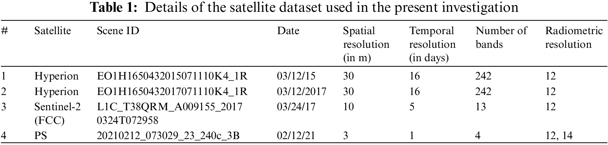
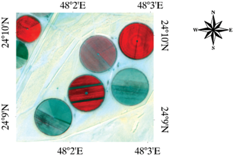
Figure 1: False-color composite of pivot fields using PS subset for Al-Kharj region on feb 02, 2021

For the assessment of super-resolution, Sentinel-2 L1-C data was used, specifically Band 4, 3, and 2, acquired in March 2017. The Sentinel-2 data underwent processing from Level-0 to Level-2. Level-0 includes preliminary quick-look and auxiliary data, while Level-1 processing consists of three steps to generate Level-1A, Level-1B, and Level-1C data. The Level-1C data, which is an orthorectified product corrected for elevation effects and provides reflectance for the top of the atmosphere, was utilized in the present investigation. It should be noted that the high spatial resolution of Sentinel VIS 10 (m) data was not available for March 2015. Therefore, the performance evaluation of the 3D-CNNHSR model was tested using the available data from March 2017, assuming it as the performance indicator.

3  Methodology

The methodology section is divided into two main sub-sections. In Section 3.1 we discussed the pre-processing of Hyperion data, Section 3.2 discussed the SR implementation using DL, and the vegetation assessment of Al Kharj based on SR images given in Section 3.3.

3.1 Hyperspectral Images Pre-Processing

Before the application of SR models, the Level-1 hyperspectral data requires preprocessing to address various conditions such as low illumination, sensor errors, noise, and atmospheric effects. The preprocessing steps involve the removal of bad bands, DN-to-radiance conversion, de-striping, and atmospheric correction. From the total of 242 continuous bands in the Hyperion dataset, 83 bands with quality issues were excluded, leaving 159 bands for further processing. Bands 1 to 7 and 225 to 242, which were not sufficiently illuminated, were removed. Additionally, bands 58 to 78 were excluded due to overlapping regions, while bands 120 to 132, 165 to 182, and 221 to 224 were eliminated due to water absorption effects.

3.1.1 De-Striping of the HSI

The calibration error of the detector array of this device causes vertical stripes in some bands. The detectors must be tuned properly to avoid stripping artifacts. Striping can produce ambiguous lines in images and variances in surrounding pixels. Strips in the images can degrade the quality of hyperspectral analysis. The local de-striping algorithm approach was used in the present investigation, it averages the striped pixel value. Local de-striping methods repaired problematic lines by averaging DN values from left and right neighbor pixels.

3.1.2 Atmospheric Correction

Hyperspectral remote sensing utilizes data from sun radiation, surface properties, and sensors. The Hyperion sensor captures the incoming solar radiation reflected from or emitted by the Earth’s surface. The interaction between the incoming radiation and atmospheric particles and gases leads to air absorption, reflectance, and scattering. In the range of 400–2500 nm, which corresponds to hyperspectral images, the atmosphere contains around thirty different gases, giving rise to atmospheric challenges. The visible region is particularly affected by molecular scattering. To address these issues, a correction technique called Fast Line-of-Sight (FLAASH) was employed. FLAASH correction involved calculating the scene-average visibility by considering various influencing factors such as sensor altitude (705 km), aerosol model (rural), K-T retrieval, beginning visibility (40.00 km), and water absorption feature (1135 nm) during the correction process.

3.1.3 MNF (Minimal Noise Fraction)

The MNF transformation was utilized to separate and equalize the noise in the data, as well as to minimize the dimensionality of data for the detection of the target. The MNF-converted data’s bands are then sorted based on the spatial coherence from higher to lower values. MNF is a PCA (principal component analysis) based on a two-step linear transformation. The first stage obtained the covariance matrix for noise to decorrelate and rescale the data noise. The equalized spectrum of the data was processed for PCA processed in the next step. To reduce noise during the data acquisition process, the inverse Minimum Noise Fraction (MNF) transformation was employed. A total of 40 MNF bands were generated based on an eigenvalue plot (Fig. 2a). The analysis of the MNF graph indicated that the first 10 MNF components provide the highest level of explanatory information.

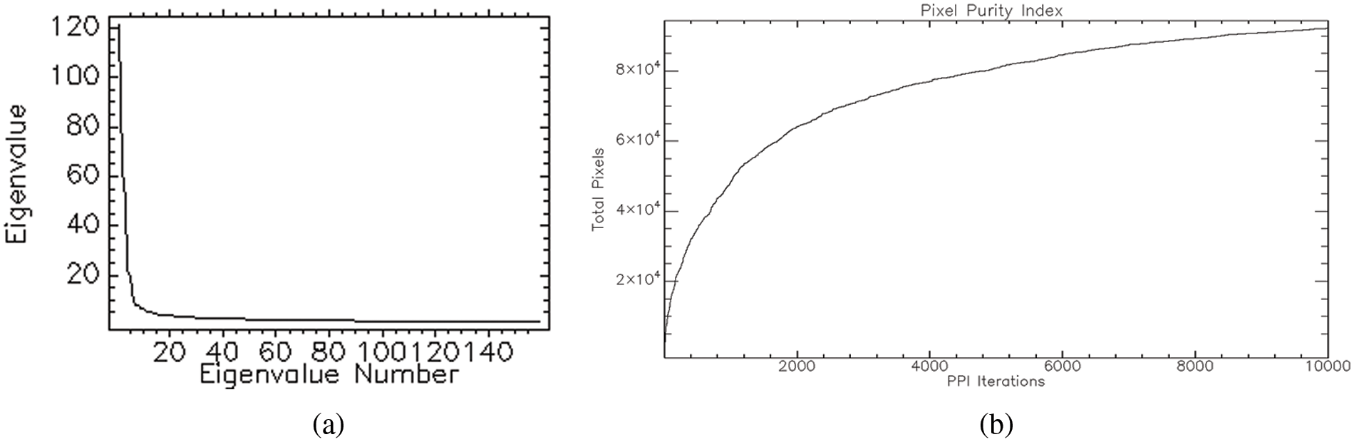
Figure 2: (a) Eigenvalue graph of MNF bands for Hyperion image of 12 march 2015; (b) shows a visualization of all pixels’ PPI iterations

3.1.4 Pixel Purity Index (PPI)

PPI is used to locate the purest pixels in a multispectral image based on the MNF images to obtain the end member spectra. The imaging spectrum is projected onto a random vector. The frequency of each pure pixel and outlier was calculated. The pixel values in the input image were transformed to threshold values, which are generally slightly higher than the noise level of the data. Finally, a PPI image is produced, with the value of each pixel showing how repeatedly a pixel has been used (Fig. 2b).

3.1.5 n-D Visualizer

The n-D Visualizer finds, identifies, and clusters the purest pixels and endmembers in an image. In n-dimensions, a PPI-based software calculation discovers and arranges the purest pixels. Finally, these pixels are used to create endmember spectra (Fig. 3a) that are input into image categorization algorithms. The 3D hypercube of the Hyperion 2015 image with the spectral profile of vegetation for a pivot field is shown in Fig. 3b.

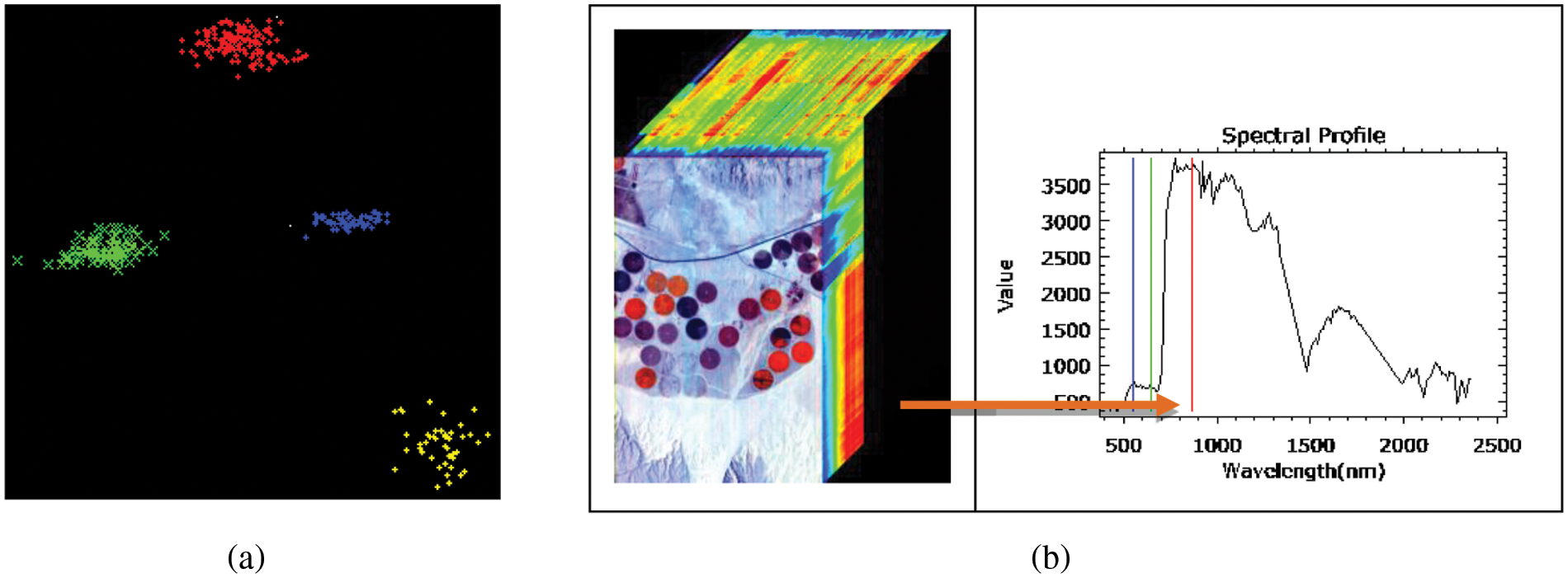
Figure 3: (a) n-D Visualizer showing endmember pixels, (Green for high vegetation, blue for less vegetation, yellow for the barren area, and red for sand); (b) 3D hypercube of Hyperion 2015 image with the spectral profile of vegetation for a pivot field indicated through the arrow

3.2 Proposed 3D-CNNHSR Model for Spatial SR

In hyperspectral applications, traditional 2D processing on HSIs can lead to spectral distortion due to the loss of spectral content encoded in compact bands. To address this, we propose using 3D convolution instead of 2D convolution, which considers both the spatial and spectral dimensions. By convolving a cube formed by clustering contiguous spectral content with a 3D kernel, we capture spatial-spectral features and mitigate spectral distortion. The 3D convolution is calculated as a weighted sum of pixels in the data cube, as described by Eq. (1).

Cabc=f(∑xyzwxyzi(a+x)(b+y)(c+z)+j)(1)

where Cabc represents the output feature at the position (a, b, c); i(a+x)(b+y)(c+z)+j) represents the input at the position (a+x)(b+y)(c+z)+j) in which (x,y,z) represents the corresponding offset of (a, b, c); wxyz represents weight. The flowchart of the methodology used in the present investigation is shown using Fig. 4.

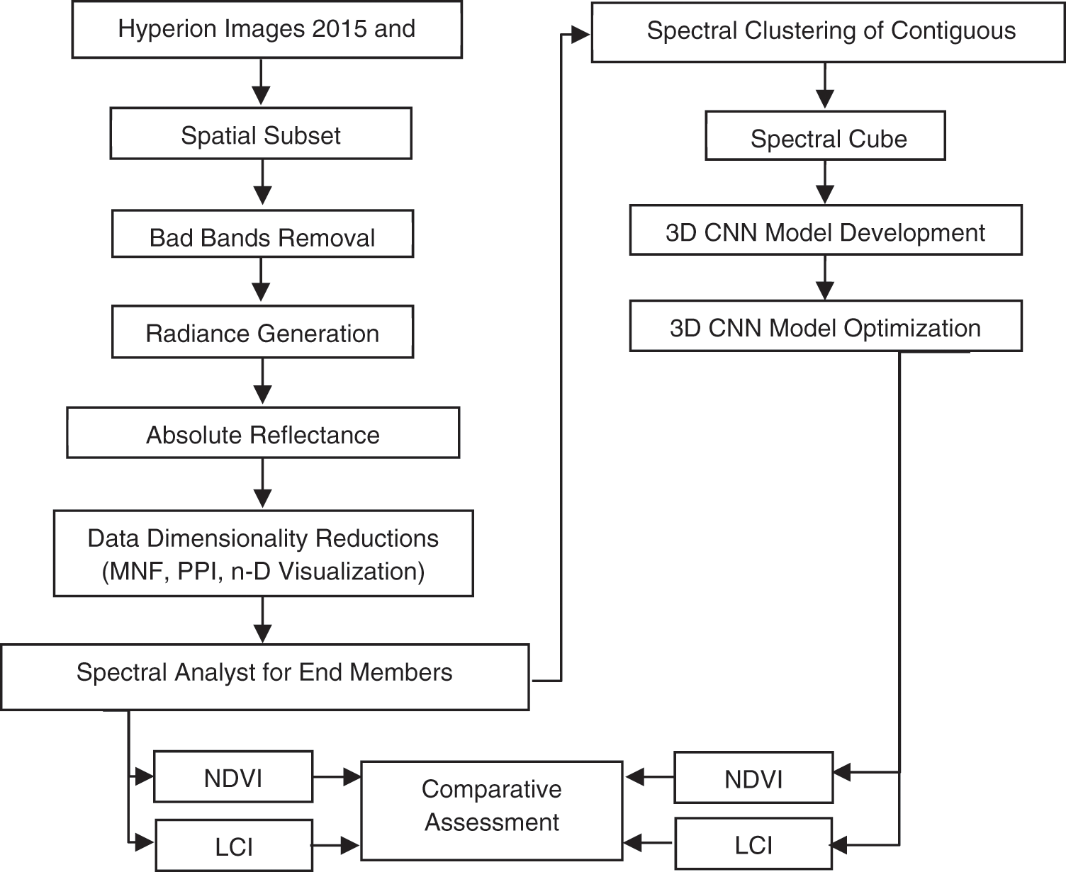
Figure 4: Flowchart of the methodology used in the present investigation

For SR of HSIs, we employed a 3D-CNNHSR, see Fig. 5. To begin, the Hyperion dataset was resampled to 15 (m) using bicubic interpolation. This resampled data was utilized to assess with 3D-CNNHSR. The interpolated images only had spatial values then the 3D convolution was utilized on the original resolution of Hyperion data to assess the unbiased performance of the developed 3D-CNNHSR model. To accomplish so, all 159 bands of pre-processed Hyperion data were fed into 3D-CNNHSR to generate a higher spatial resolution of 15 meters resulting in a Hyperion image, which also contains high spectral resolution.

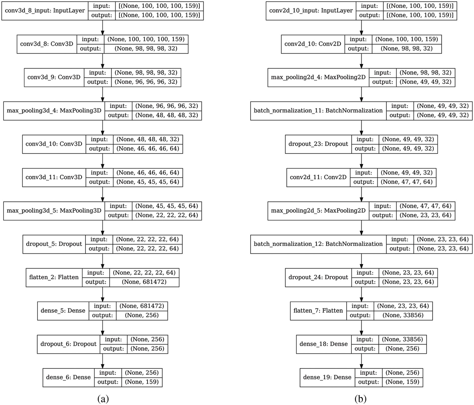
Figure 5: Architecture of the SR models (a): 3D-CNNHSR model; (b) 2D CNN model

The proposed 3D-CNNHSR has seven layers, with four convolutional layers, and three fully connected dense layers, the output of the entire network was obtained through the final layer with the softmax function. The number of neurons in a CNN depends on the parameters, however, in SR applications, the initial result has a large impact on the network’s scalability due to higher dimensionality. A subset of 100 × 100 pixels was fed to the 3D-CNNHSR model and a 3D kernel which is also known as a filter or feature detector was used. The term “feature map” refers to a feature that has been convolved. As a result, all the convolution layers’ filters are programmed to learn spectral information from contiguous spectral bands. We employ the ReLU activation function to control the linearity after the convolution layer since features in HSI images are nonlinear generally. Four convolution layers were added, resulting in the volume of information shrinking faster, therefore, to preserve as much information in the early layers of our network padding was utilized. The maxpool function was used to enable the sub-sampling or down-sampling by reducing the parameters, which makes feature detection insensitive to changes in scale or orientation [46]. Dropouts were also used to reduce the effect of overfitting by disconnecting neurons in the different layers. Finally, all activations from previous layers were connected to neurons in the fully connected layer. The 3D-CNNHSR model was compared and evaluated against the four layers of the 2D-CNN model (Fig. 5). The batch dimension is denoted by the none dimension in the shape tuple (Fig. 5), which indicates that the layer can accept input of any size. e.g., MNIST dataset might have the shape tuple (60000, 28, 28, 1), however, the shape of the input layer would be (None, 28, 28, 1). The dimensions of the input shape for the 3D-CNNHSR model were four i.e., (100, 100, 100, 159). A three-dimensional image is a four-dimensional data set, with the fourth dimension representing the number of channels. The input of the 2D-CNN model has three dimensions (100, 100, 159), and the third dimension represents color channels and 4 layers of 2D convolution with 4 dropout layers to control overfitting.

3.3 Vegetation Assessment for AL Kharj Area

3.3.1 NDVI

The NDVI index is an index of plant “greenness” or photosynthetic activity that is based on the photosynthetic process of vegetation [7,9,33]. The NDVI method was based on the idea that plants absorb the red light essential for photosynthesis but reflect the light in the NIR region.

The following equation can be used to calculate NDVI (2).

NDVI=λ(854)−λ(650)λ(854)+λ(650)(2)

The Normalized Difference Vegetation Index (NDVI) is influenced by various factors such as vegetation density, vegetation stress, and soil exposure. Being a ratio-based index, NDVI offers several benefits, including the ability to account for topographic lighting variations and facilitate multi-temporal image analysis for comparing images captured in different seasons.

3.3.2 LCI

The LCI was found to be a sensitive measure of chlorophyll content in leaves that were less impacted by scattering from the surface of the crop and interior structure variations [46]. LCI is defined as the proportion of relative chlorophyll absorption intensities in the NIR and red edge and red wavelengths, Eq. (3).

LCI=λ(854)−λ(711)λ(854)+λ(681)(3)

The value of LCI grows as the amount of leaf chlorophyll in the leaf increases. The LCI was developed using the pre-processed bands of HSI including 43, 29, and 26. The wavelengths of these bands are 854, 711, and 681 nm, respectively.

4  Performance Evaluation

To assess the quality of the SR results, various performance metrics were employed, including the mean peak signal-to-noise ratio (MPSNR), mean square error (MSE), and the mean structural similarity (MSSIM) index. These metrics were selected as they are well-suited for effectively evaluating image quality [21]. The SR images generated from the Hyperion dataset were compared against the Sentinel-2 data, which has a ground truth spatial resolution of 10 meters. The mean structural similarity index measure (MSSIM) was utilized as a technique to estimate the relative quality of digital images. It measures the similarity between two images, providing an assessment of image quality by comparing the SR results with a high-resolution ground truth image.

MSE and MPSNR, calculate absolute errors, whereas these MSSIM methods measure relative errors. The MPSNR can be given as Eq. (4).

MPSNR=1p∑i=0p10×log10(BV(max)x2MSEx)(4)

where BV(maxx) is the pixel with the highest value in the xth band, and MSEx represents the MSE of the xth band. MSE can be calculated as Eq. (5).

MSE=1t∑i=0t(1lbp ∑x=0l(∑y=0b∑z=0p(Bxyz−R(A)xyz)))(5)

where t, l, and b, represent training samples, the output length of R(A), and the breadth of the output respectively. The MSSIM between ground truth B of the reconstructed image R(A) can be defined as Eq. (6).

MSSIM=1p∑i=0p(2μR(A)iμYi+p1)(2σR(A)iBi+p2)(μR(A)i2+μBi2+p1)(σR(A)i2+σBi2+p2)(6)

where  R(A)i and Bi is the xth band of R(A) and B, notations with μ and σ represent the mean and variance values of associated bands.

5  Results and Discussion

Hyperion images for March 12, 2015, and March 12, 2017, before and after super-resolution (below) using 3D-CNNHSR were shown in Figs. 6–8. Based on visual inspection it was observed that the spatial quality of Hyperion data was improved using 3D-CNNHSR. The features such as some premises which were blurred in the original Hyperion data were improved and detectable after super-resolution. Furthermore, to verify the performance of the 3D-CNNHSR for spatial SR of HSIs rigorous experiments were performed. Due to the unavailability of higher resolution data for March 2015 in the public domain; it was assumed that the assessment of the developed model was consistent for both years i.e., 2015 and 2017. The developed model was tested on various land use/landcover classes including vegetation area. The parameters of the 3D-CNNHSR model were also assessed for various combinations of neurons and kernel filters. The outputs of the models were computed by fixing the number of layers as constant while changing the filters continuously and then comparing them to see which condition the model performed best in. An important observation was that LCI generate better results for vegetation classification assessed using Sentinel-2 data of 24 March 2017 for Hyperion 12 March 2017 image. It was observed based on vegetation indices analysis that LCI performs better than NDVI due to the saturation behavior of NDVI in scattered vegetation and exposed soil reflectance. In general, a higher mean peak signal-to-noise ratio (MPSNR) and mean structural similarity (MSSIM) value indicate better visual quality, while a lower Spectral Angle Mapper (SAM) value indicates reduced spectral distortion and higher quality of spectral reconstruction (refer to Table 2).

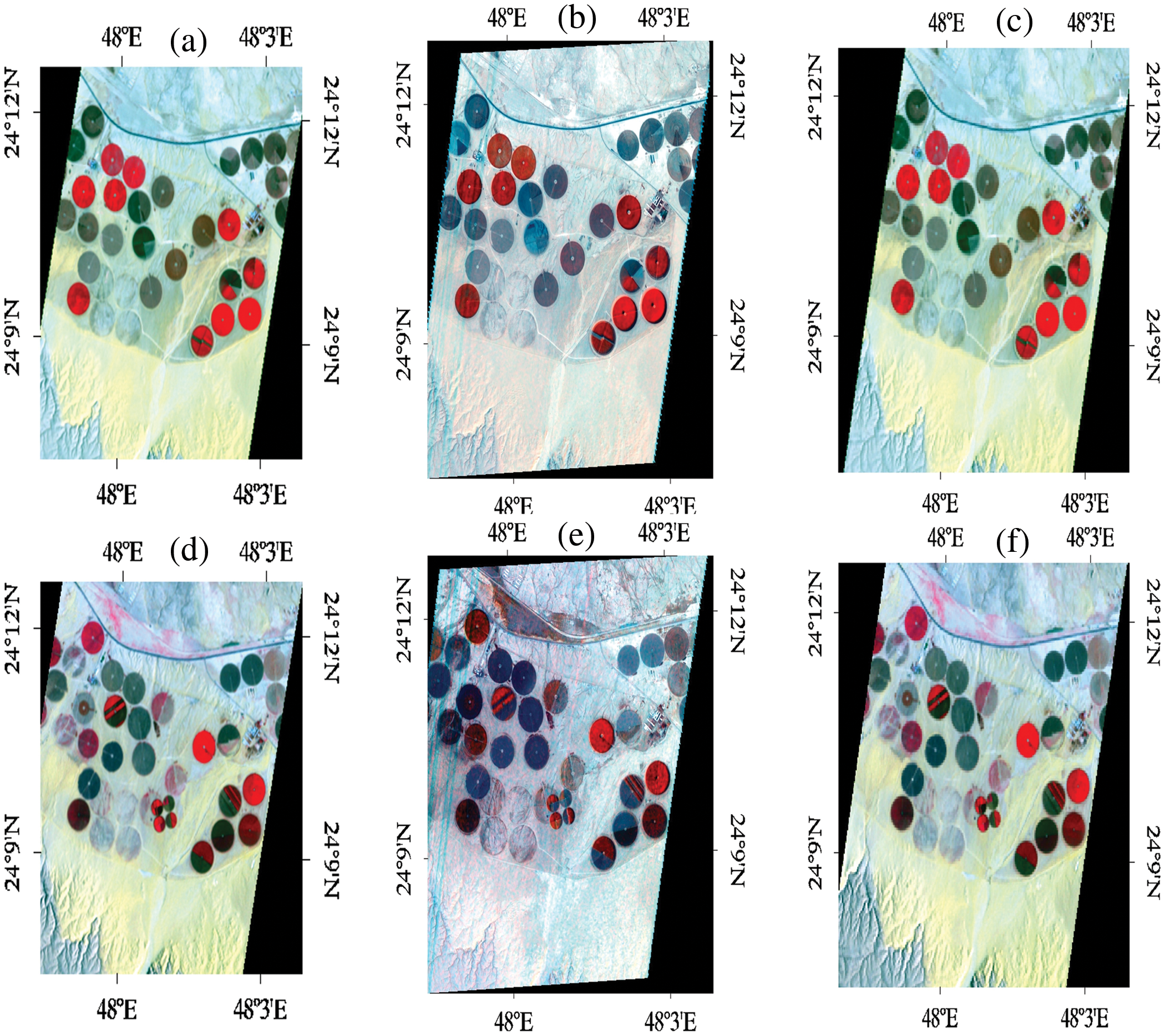
Figure 6: (a) Hyperion image of march 12, 2015; (b) output of 3DCNNHSR; (c) output of 2D CNN; (d) Hyperion image of march 12, 2017; (e) output of 3DCNNHSR; (f) output of 2D CNN

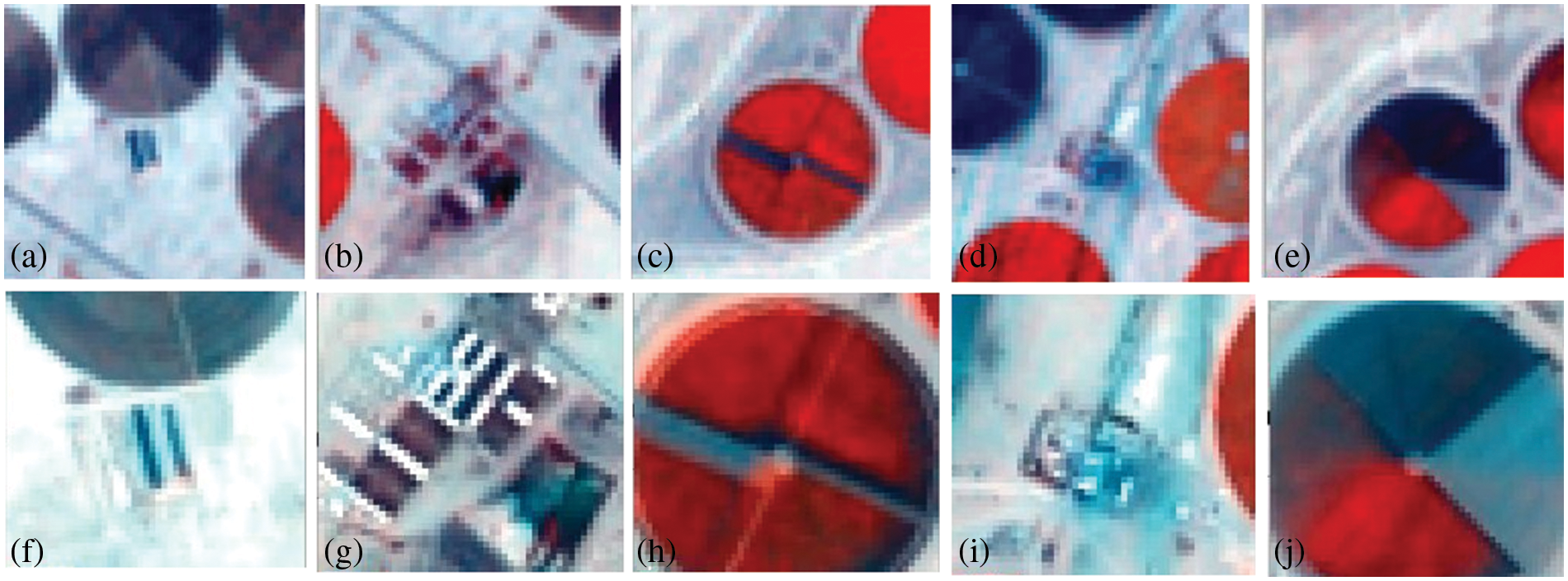
Figure 7: Hyperion image of march 12, 2015, pre (a–e) and after (f–j) applying the 3D-CNNHSR model

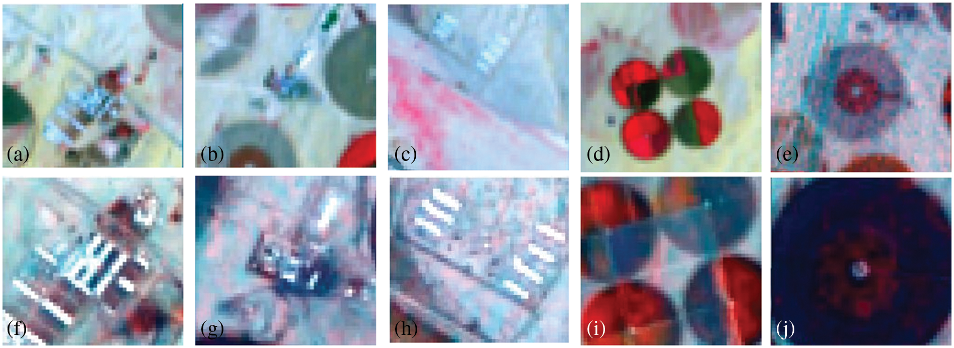
Figure 8: Hyperion image of march 12, 2017, pre (a–e) and after (f–j) applying the 3D-CNNHSR model

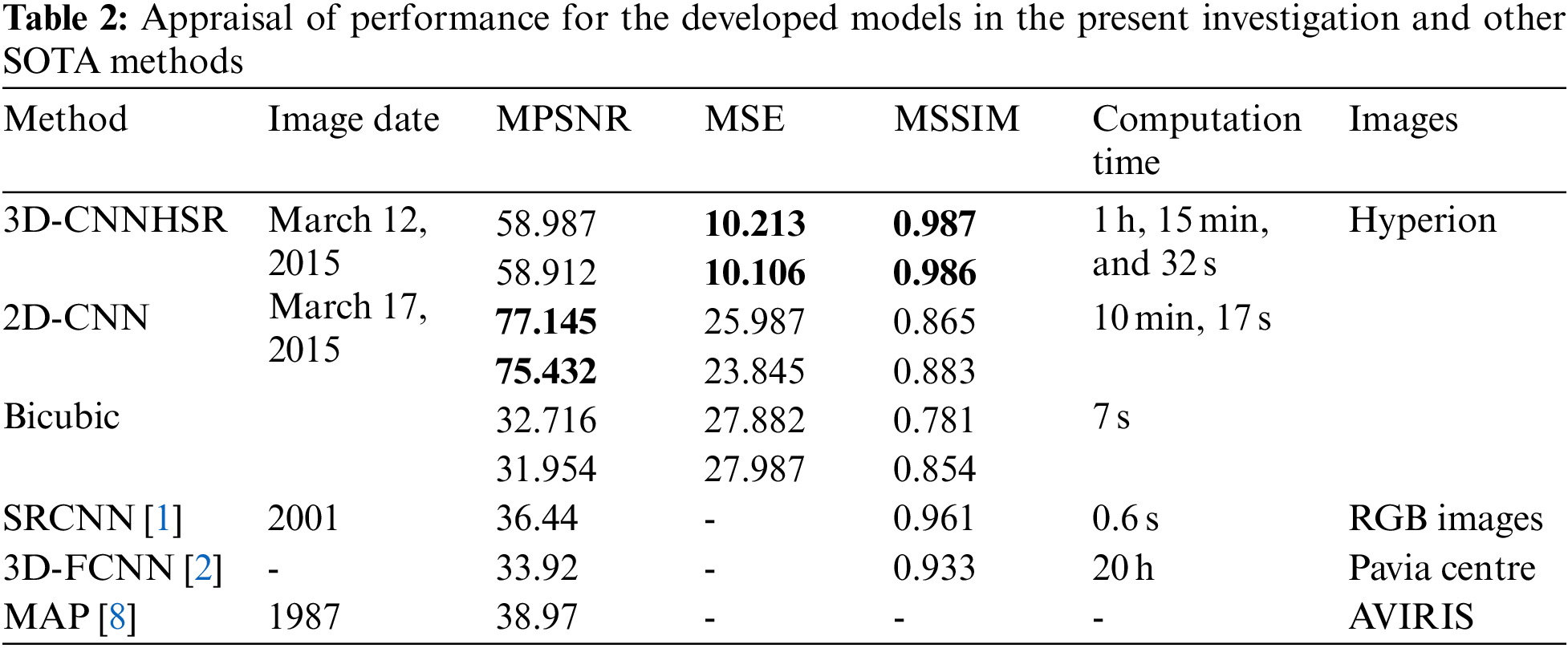
The performance of the 3D-CNNHSR was compared with the 2D-CNN model and bicubic interpolation. It was observed that the 3D-CNNHSR model outperformed the 2D-CNN model and bicubic based on MSE, and MSSIM values. Furthermore, because the 2D-CNN has fewer parameters of 8,838,751 which is 33 times lesser than the 293,554,979 parameters for 3D-CNNHSR, training is significantly faster for the 2D-CNN model. However, the 3D-CNNHSR model outperforms not only based on evaluation metrics but also because the visual quality of the images was higher, see Fig. 6. The 3D-CNNHSR model output seems better than the original image while the 2D-CNN output looks blurry compared to the 3D-CNNHSR model output. The results of the present study were also compared with earlier studies for assessment. It was observed that the present model outperformed the 3D-FCNN model developed by [2], based on MPSNR and MSSIM values. The highest value obtained by [2] for PSNR was 0.969 however present study achieved the PSNR values of 0.987 and 0.986 for the data of 2015 and 2017, respectively. The MPSNR value achieved by [2] was 33.92 using pre-processed Pavia dataset; however present investigation used raw data and converted it to a low-noise dataset after performing rigorous pre-processing steps before feeding to a 3D-CNNHSR model and achieving better PSNR values.

6  Computational Efficiency

The developed 3D-CNNHSR model converges faster using callback functions and an automated and optimal number of epochs. The 3D-CNNHSR model had 293,554,979 parameters, while the 2D-CNN model has fewer parameters 8,838,751 which is 33 times lesser than the 3D-CNNHSR. The training is significantly faster for the 2D-CNN model. However, the 3D-CNNHSR model outperforms not only based on evaluation metrics but also the visual quality of the images was higher. The computational complexity for 3D-CNNHSR and 2D-CNN were O (n6) and O (n4), respectively. The current study made use of TPUs (Tensor Processing Units) v2–8. These TPUs are application-specific circuits developed by Google. It speeds up the training operations for AI models using eight cores and 64 GB of memory. The TPU v2–8 that was used in this study with 68 epochs, 3D-CNNHSR took 1 h, 15 min, and 32 s for training (Fig. 9a), which is quite lesser compared to the 20 h taken by [2]. Additionally, [2] used very smaller image sizes including 33 × 33, 44 × 44, and 55 × 55; however present investigation took images 100 × 100 in size for training. The model developed by [2] has fewer parameters of 88907 based on the smaller image size used for training however the MPSNR value (34.03) was low compared to higher MPSNR values of 58.987 and 58.912 using 3D-CNNHSR for 2015 and 2017, respectively. Bicubic interpolation, on the other hand, took only 7 s and 32 milliseconds to perform the image resampling using the same system specifications, however, it yields a low MPSNR of 32 and a high MSE. The relationship between the 3D-CNNHSR model’s loss and the epoch number is shown in Fig. 9a. As the number of epochs increases, i.e., as learning develops, the loss values drop. The model’s loss patterns were different when the hyperparameters of the 3D-CNNHSR were changed. According to the analysis, some models lose weight swiftly, while others lose weight gradually. Before calculating the learning, rate and putting it to the test by modifying the layers for the Al-Kharj photos using 3D-CNNHSR, we tried 7 layers with different learning rates. Among the various combinations, the model with 7 layers and 0.05 lr performed best, as shown in Fig. 9b.

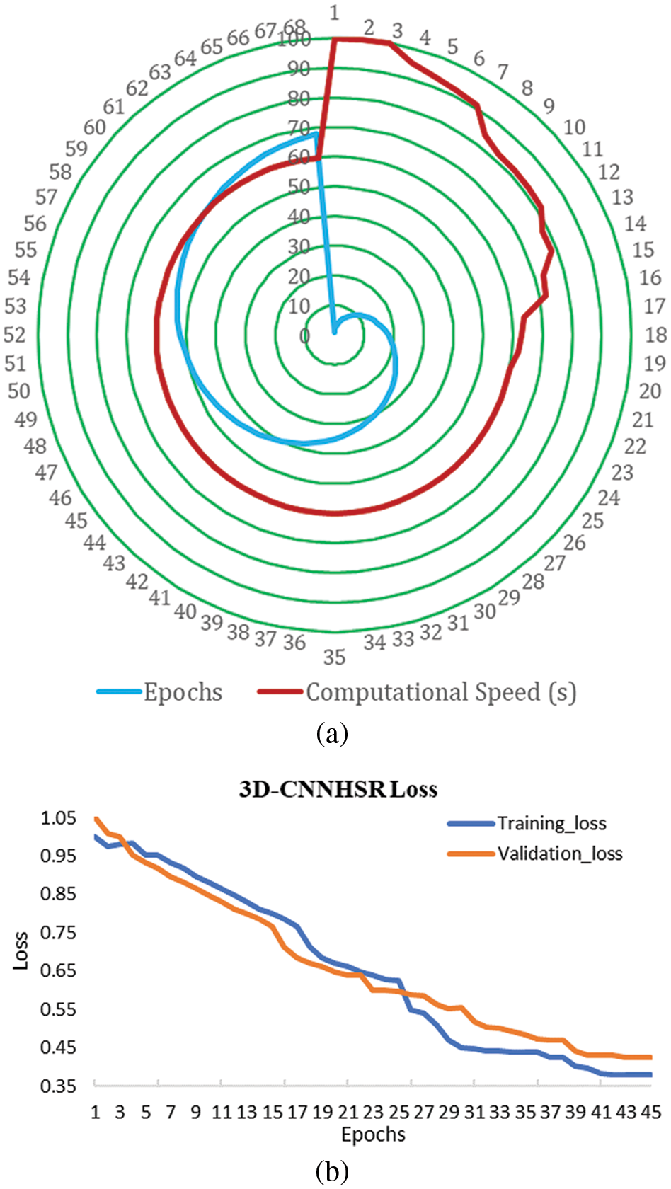
Figure 9: (a) Computational speed of the 3D-CNNHSR model; (b) loss with epochs for the 3D-CNNHSR model

7  Conclusion

In this paper, we have addressed the issue of low spatial resolution of a hyperspectral dataset based on the developed and optimized 3D-CNNHSR model for super-resolution. Hyperspectral pre-processing was performed systematically before applying the 3D-CNNHSR model so that the noise can be minimized, and the SNR can be improved. The bands of the Hyperion dataset were reduced to 159 from a total of 242 bands after pre-processing. The super-resolution was applied for all 159 bands. The performance of the 3D-CNNHSR was evaluated using MPSNR, MSE, and MSSIM metrics based on the Sentinel-2 dataset which contains a 10 m resolution. The developed model has shown a high MPSNR of 58.987 and 58.912 for Hyperion 2015 and Hyperion 2017 SR images, respectively. MSSIM suggested that the 3D-CNNHSR model achieved the value of 0.987 and 0.986 for the March 2015 and March 2017 SR images. The computational speed of the 3D-CNNHSR model was found promising using the TPU v2–8 with 68 epochs, 3D-CNNHSR took 1 h, 15 min, and 32 s for training, which is quite lesser compared to the previous studies. The SR images were utilized for assessing the vegetation of the Al-Kharj area based on NDVI and LCI. Additionally, it was observed that LCI performed better than NDVI in an arid area of Al-Kharj. The future scope of the present investigation is to assess and optimize the 3D-CNNHSR for other domains [47].

Acknowledgement: The authors extend their appreciation to the Deanship of Scientific Research at King Khalid University for funding this work through large group Research Project under Grant Number RGP2/80/44.

Funding Statement: The authors extend their appreciation to the Deanship of Scientific Research at King Khalid University for funding this work through large group Research Project under Grant Number RGP2/80/44.

Conflicts of Interest: The authors declare that they have no conflicts of interest to report regarding the present study.

References

1. C. Dong, C. C. Loy, K. He and Tang X., “Image super-resolution using deep convolutional networks,” IEEE Transactions on Pattern Analysis and Machine Intelligence, vol. 38, no. 2, pp. 295–307, 2016. [Google Scholar] [PubMed]

2. S. Mei, X. Yuan, J. Ji, Y. Zhang, S. Wan et al., “Hyperspectral image spatial super-resolution via 3D full convolutional neural network,” Remote Sensing, vol. 9, no. 11, pp. 1139, 2017. [Google Scholar]

3. J. Li, J. M. Bioucas-Dias and A. Plaza, “Spectral-spatial hyperspectral image segmentation using subspace multinomial logistic regression and Markov random fields,” IEEE Transactions on Geoscience and Remote Sensing, vol. 50, no. 3, pp. 809–823, 2012. [Google Scholar]

4. B. Du and L. Zhang, “A discriminative metric learning based anomaly detection method,” IEEE Transactions on Geoscience and Remote Sensing, vol. 52, no. 11, pp. 6844–6857, 2014. [Google Scholar]

5. K. Tan, X. Jin, A. Plaza, X. Wang, L. Xiao et al., “Automatic change detection in high-resolution remote sensing images by using a multiple classifier system and spectral-spatial features,” IEEE Journal of Selected Topics in Applied Earth Observations and Remote Sensing, vol. 9, no. 8, pp. 3439–3451, 2016. [Google Scholar]

6. S. Asadzadeh, C. Roberto and D. S. Filho, “A review on spectral processing methods for geological remote sensing,” International Journal of Applied Earth Observation and Geoinformation, vol. 47, pp. 69–90, 2016. [Google Scholar]

7. D. Zhang, H. Pu, F. Li, X. Ding and V. S. Sheng, “Few-shot object detection based on the transformer and high-resolution network,” Computers, Materials & Continua, vol. 74, no. 2, pp. 3439–3454, 2023. [Google Scholar]

8. R. C. Hardie, M. T. Eismann and G. L. Wilson, “Map estimation for hyperspectral image resolution enhancement using an auxiliary sensor,” IEEE Transactions on Image Processing, vol. 13, no. 9, pp. 1174–1184, 2004. [Google Scholar] [PubMed]

9. M. A. Haq, “Planetscope nanosatellites image classification using machine learning,” Computer Systems and Science Engineering, vol. 42, no. 3, pp. 1031–1046, 2022. [Google Scholar]

10. M. T. Eismann and R. C. Hardie, “Hyperspectral resolution enhancement using high-resolution multispectral imagery with arbitrary response functions,” IEEE Transactions on Geoscience and Remote Sensing, vol. 43, no. 3, pp. 455–465, 2005. [Google Scholar]

11. K. Nirmal and M. John, “Spectral unmixing. signal processing magazine,” IEEE Magzine, vol. 19, no. 1, pp. 44–57, 2002. [Google Scholar]

12. E. M. T. Hendrix, I. Garcia, J. Plaza, G. Martin and A. Plaza, “A new minimum-volume enclosing algorithm for endmember identification and abundance estimation in hyperspectral data,” IEEE Transactions on Geoscience and Remote Sensing, vol. 50, no. 7, pp. 2744–2757, 2012. [Google Scholar]

13. A. Huck, M. Guillaume and J. Blanc-Talon, “Minimum dispersion constrained nonnegative matrix factorization to unmix hyperspectral data,” IEEE Transactions on Geoscience and Remote Sensing, vol. 48, no. 6, pp. 2590–2602, 2010. [Google Scholar]

14. Y. Qian, S. Jia, J. Zhou and A. Robles-Kelly, “Hyperspectral unmixing via l1/2 sparsity-constrained nonnegative matrix factorization,” IEEE Transactions on Geoscience and Remote Sensing, vol. 49, no. 11, pp. 4282–4297, 2011. [Google Scholar]

15. S. Mei, M. He, Z. Wang and D. D. Feng, “Unsupervised spectral mixture analysis of highly mixed data with hopfield neural network,” IEEE Journal of Selected Topics in Applied Earth Observations and Remote Sensing, vol. 7, no. 6, pp. 1922–1935, 2014. [Google Scholar]

16. D. Manolakis, C. Siracusa and G. Shaw, “Hyperspectral subpixel target detection using the linear mixing model,” IEEE Transactions on Geoscience and Remote Sensing, vol. 39, no. 7, pp. 1392–1409, 2001. [Google Scholar]

17. L. Zhang, L. Zhang, D. Tao, X. Huang and B. Du, “Hyperspectral remote sensing image subpixel target detection based on supervised metric learning,” IEEE Transactions on Geoscience and Remote Sensing, vol. 52, no. 8, pp. 4955–4965, 2014. [Google Scholar]

18. Y. Tang, Z. Pan, W. Pedrycz, F. Ren and X. Song, “Viewpoint-based kernel fuzzy clustering with weight information granules,” IEEE Transactions on Emerging Topics in Computational Intelligence, vol. 7, pp. 1–15, 2022. [Google Scholar]

19. P. M. Atkinson, “Mapping subpixel boundaries from remotely sensed images,” in Innovations in GIS, vol. 4. London, UK: Taylor and Francis, pp. 166–180, 1997. [Google Scholar]

20. G. M. Foody, “Sharpening fuzzy classification output to refine the representation of sub-pixel land cover distribution,” International Journal of Remote Sensing, vol. 19, no. 13, pp. 2593–2599, 1998. [Google Scholar]

21. Z. Wang, A. C. Bovik, H. R. Sheikh and E. P. Simoncelli, “Image quality assessment: From error visibility to structural similarity,” IEEE Transactions on Image Processing, vol. 13, no. 4, pp. 600–612, 2004. [Google Scholar] [PubMed]

22. K. C. Mertens, D. B. Baets, L. Verbeke and D. R. Wulf, “A sub-pixel mapping algorithm based on sub-pixel/pixel spatial attraction models,” International Journal of Remote Sensing, vol. 27, pp. 3293–3310, 2006. [Google Scholar]

23. P. Atkinson, “Sub-pixel target mapping from soft-classified, remotely sensed imagery,” Photogrammetric Engineering and Remote Sensing, vol. 71, no. 7, pp. 839–846, 2005. [Google Scholar]

24. L. C. Pickup, D. P. Capel, S. J. Roberts and A. Zisserman, “Bayesian image super-resolution, continued,” Advance in Neural Information and Processing Systems, vol. 19, pp. 1089–1096, 2006. [Google Scholar]

25. X. Xu, Y. Zhong, L. Zhang and H. Zhang, “Sub-pixel mapping based on a map model with multiple shifted hyperspectral imagery,” IEEE Journal of Selected Topics in Applied Earth Observations and Remote Sensing, vol. 6, no. 2, pp. 580–593, 2013. [Google Scholar]

26. T. Kasetkasem, M. K. Arora and P. K. Varshney, “Super-resolution land cover mapping using a Markov random field based approach,” Remote Sensing of Environment, vol. 96, pp. 302–314, 2005. [Google Scholar]

27. L. Wang and Q. Wang, “Subpixel mapping using markov random field with multiple spectral constraints from subpixel shifted remote sensing images,” IEEE Geoscience and Remote Sensing Letters, vol. 10, no. 3, pp. 598–602, 2013. [Google Scholar]

28. F. Ling, Y. Du, F. Xiao, H. Xue and S. Wu, “Super-resolution land-cover mapping using multiple sub-pixel shifted remotely sensed images,” International Journal of Remote Sensing, vol. 31, pp. 5023–5040, 2010. [Google Scholar]

29. K. C. Mertens, L. P. C. Verbeke, T. Westra and D. R. Wulf, “Subpixel mapping and sub-pixel sharpening using neural network predicted wavelet coefficients,” Remote Sensing of Environment, vol. 91, pp. 225–236, 2004. [Google Scholar]

30. A. J. Tatem, H. G. Lewis, P. M. Atkinson and M. S. Nixon, “Super-resolution land cover pattern prediction using a Hopfield neural network,” Remote Sensing of Environment, vol. 79, pp. 1–14, 2002. [Google Scholar]

31. A. Villa, J. Chanussot, J. A. Benediktsson and C. Jutten, “Spectral unmixing for the classification of hyperspectral images at a finer spatial resolution,” IEEE Journal of Selected Topics in Signal Processing, vol. 5, no. 3, pp. 521–533, 2011. [Google Scholar]

32. R. Feng, Y. Zhong, X. Xu and L. Zhang, “Adaptive sparse subpixel mapping with a total variation model for remote sensing imagery,” IEEE Transactions on Geoscience and Remote Sensing, vol. 54, no. 5, pp. 2855–2872, 2016. [Google Scholar]

33. Y. Zhang, Y. Du, F. Ling, S. Fang and X. Li, “Example-based super-resolution land cover mapping using support vector regression,” IEEE Journal of Selected Topics in Applied Earth Observations and Remote Sensing, vol. 7, no. 4, pp. 1271–1283, 2014. [Google Scholar]

34. Y. C. Shekhar, M. K. Pradhan, S. M. P. Gangadharan, J. K. Chaudhary, J. Singh et al., “Multi-class pixel certainty active learning model for classification of land cover classes using hyperspectral imagery,” Electronics, vol. 11, no. 17, pp. 2799, 2022. [Google Scholar]

35. M. Anul Haq, A. Khadar Jilani and P. Prabu, “Deep learning based modeling of groundwater storage change,” Computers, Materials & Continua, vol. 70, no. 3, pp. 4599–4617, 2022. [Google Scholar]

36. M. Anul Haq, “Cnn based automated weed detection system using uav imagery,” Computer Systems Science and Engineering, vol. 42, no. 2, pp. 837–849, 2022. [Google Scholar]

37. L. Z. Pen, K. X. Xian, C. F. Yew, O. S. Hau, P. Sumari et al., “Artocarpus classification technique using deep learning based convolutional neural network,” in Classification Applications with Deep Learning and Machine Learning Technologies, vol. 1071. NY, USA, Cham: Springer International Publishing, pp. 1–21, 2023. [Google Scholar]

38. C. Ke, N. T. Weng, Y. Yang, Z. M. Yang, P. Sumari et al., “Mango varieties classification-based optimization with transfer learning and deep learning approaches,” in Classification Applications with Deep Learning and Machine Learning Technologies, vol. 1071. NY, USA, Cham: Springer International Publishing, pp. 45–65, 2023. [Google Scholar]

39. L. W. Theng, M. M. San, O. Z. Cheng, W. W. Shen, P. Sumari et al., “Salak image classification method based deep learning technique using two transfer learning models,” in Classification Applications with Deep Learning and Machine Learning Technologies, vol. 1071. NY, USA, Cham: Springer International Publishing, pp. 67–105, 2023. [Google Scholar]

40. A. Abdo, C. J. Hong, L. M. Kuan, M. M. Pauzi, P. Sumari et al., “Markisa/passion fruit image classification based improved deep learning approach using transfer learning,” in Classification Applications with Deep Learning and Machine Learning Technologies, vol. 1071. NY, USA, Cham: Springer International Publishing, pp. 143–189, 2023. [Google Scholar]

41. Y. Zhang, J. Chu, L. Leng and J. Miao, “Mask-Refined R-CNN: A network for refining object details in instance segmentation,” Sensors, vol. 20, no. 4, pp. 1010, 2020. [Google Scholar] [PubMed]

42. T. Wu, L. Leng and K. Khan, Artificial Intelligence Reviews, vol. 56, pp. 6169–6186, 2022. [Google Scholar]

43. T. Wu, L. Leng, M. K. Khan and F. A. Khan, “Palmprint-palmvein fusion recognition based on deep hashing network,” IEEE Access, vol. 9, pp. 135816–135827, 2021. [Google Scholar]

44. J. Chu, Z. Guo and L. Leng, “Object detection based on multi-layer convolution feature fusion and online hard example mining,” IEEE Access, vol. 6, pp. 19959–19967, 2018. [Google Scholar]

45. M. A. Haq, “CDLSTM: A novel model for climate change forecasting,” Computers, Materials & Continua, vol. 71, no. 2, pp. 2363–2381, 2022. [Google Scholar]

46. Q. Wei, J. Bioucas-Dias, N. Dobigeon and J. Y. Tourneret, “Hyperspectral and multispectral image fusion based on a sparse representation,” IEEE Transactions on Geoscience and Remote Sensing, vol. 53, no. 7, pp. 3658–3668, 2015. [Google Scholar]

47. M. A. Haq, “Smotednn: A novel model for air pollution forecasting and aqi classification,” Computers, Materials & Continua, vol. 71, no. 1, pp. 1403–1425, 2022. [Google Scholar]