Knee Osteoarthritis Classification Using X-Ray Images Based on Optimal Deep Neural Network

1  Introduction

For older adults, knee osteoarthritis (KOA) is the most severe cause of disability [1]. Knee joint disease is caused by the deterioration of ligament tissues among knee bones (Fibula, Tibia, and Femur). According to the World Health Organization (WHO) report, 28% of people over sixty suffer from KOA. Of those, 80% have severe issues, while 25% cannot perform daily tasks [2]. According to recent studies, KOA will impact at least 130 million individuals by 2050 as the world’s population ages [3]. However, diagnosis of KOA is not easy as multiple factors affect the causes of the disease, such as age, gender, hormones, genetics, and Body Mass Index (BMI). In the worst case, scenario patient with KOA may have to go through a whole knee replacement [4]. However, early detection of knee joint disease may help older people regain mobility.

Interrogating the radiographs such as X-Ray images is a common method to diagnose the disease [5]. Radiographs (X-rays) remain the gold standard for KOA screening due to their expense, protection, wide availability, and timeliness. According to radiologists, joint space narrowing (JSN) and osteophyte development, as seen in Fig. 1, are the most conspicuous pathological characteristics of KOA. Using the Kellgren-Lawrence (KL) grading system, these two characteristics can also be utilized to assess the severity of KOA [6]. Using this method, KOA severity is graded into five categories, ranging from grade 0 to grade 4, based on the agreed ground truth categorization [7].

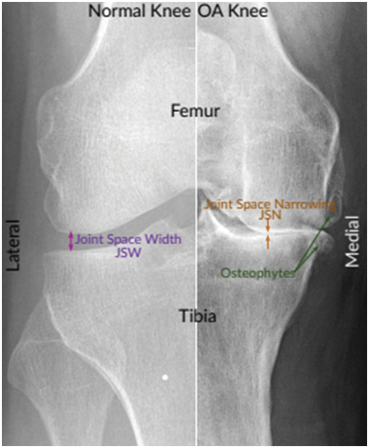
Figure 1: Normal and severe osteoarthritic knee [8]

Grade 0 indicates healthy joints where the radiological characteristics of knee osteoarthritis are absent. Grade 1 KOA indicates the likelihood of osteophytic lip and dubious JSN. Grade 2 OA is characterized by the existence of osteophytes and the potential of JSN [9]. The presence of JSN, numerous osteophytes, and sclerosis characterizes grade 3 OA. Finally, grade 4 indicates severe OA due to massive osteophytes within the joints, as shown by JSN and extensive sclerosis. Fig. 2 depicts knee joint specimens from each KL grade.

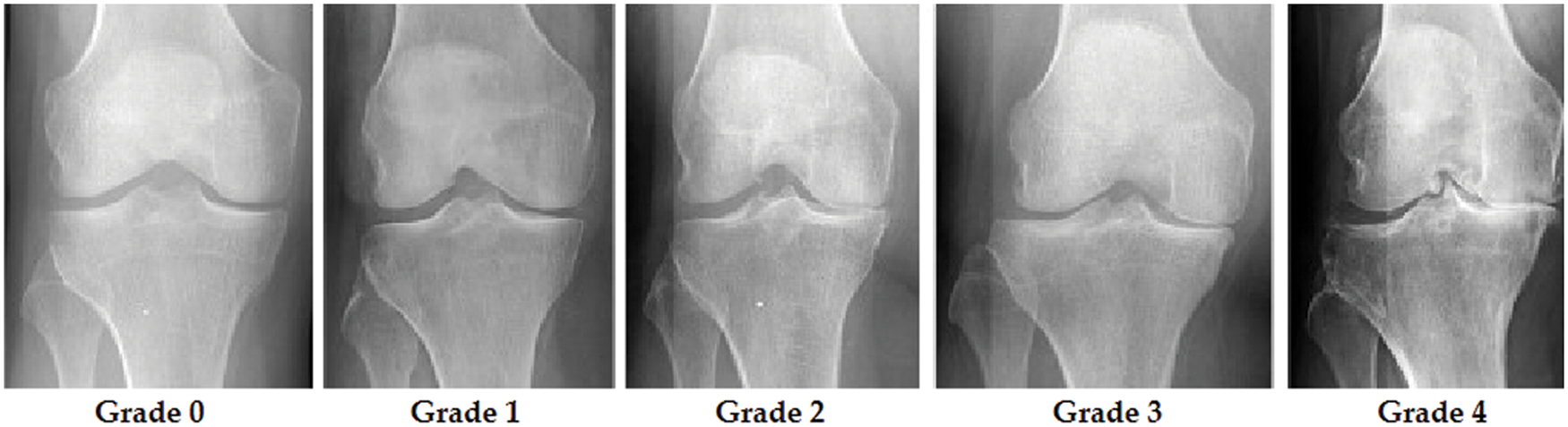
Figure 2: KOA levels according to KL grades

Due to the scarcity of radiologists, particularly in remote locations, and the duration of time necessary to examine knee X-ray images, entirely automated categorization of knee stiffness is in high demand as it expedites the diagnostic method and improves the rate of earlier recognition [10]. To identify and assess KOA, several computer-aided diagnostics (CAD) based clinical imaging systems have been presented in the scientific literature [11].

To quantify the severity of knee joint osteoarthritis, some detection methods based on deep learning have been developed and effectively used [12]. In addition, the authors provide astounding effectiveness in assessing X-rays images in the biomedical field without requiring human feature extraction, which occurs implicitly during the training stage by adjusting its hyperparameters to match the relevant data. On the other hand, all typical Machine Learning (ML) techniques demand that the provided data be changed using a specific feature engineering or training methodology before producing the intended results [13]. As a result, deep Learning (DL) methods often need a disproportionate amount of processing capacity and resources compared to normal ML techniques [14]. In addition, it leads to overfitting if limited data are provided. Moreover, some types of DL, such as Resnet, Inception, Xception, and CNN-based on Transfer Learning (TL) [15], achieve exceptional efficiency in computer vision, surpassing that of humans [16].

Deep feature extraction is crucial because it enables the automated learning and extraction of useful, high-level features from raw data [17]. This is beneficial in many cases where hand-crafted features are difficult to build or insufficiently expressive to represent the underlying data patterns. Deep feature extraction can also increase the performance of downstream models and eliminate the need for human feature engineering, resulting in more scalable and efficient solutions. Feature fusion is a process in machine learning where multiple sources of information or features are combined to form a new, more informative representation of the data. The curse of dimensionality pertains to the complications that occur while interacting with high-dimensional data. Dimensionality reduction or feature selection can be utilized to overcome the curse of dimensionality. Feature selection aids in enhancing model precision, minimizing overfitting, reducing training time, and enhancing interpretability [18]. It also assists in identifying the most significant attributes by eliminating excessive or redundant features that may enhance throughput and a more accurate generalization of new data.

Major Contributions: This article proposed a new framework for classifying knee osteoarthritis using deep learning and optimal feature selection. Our major contributions consist of the following:

•   The dataset is preprocessed using Brightness Preserving Histogram Equalization (BPHE).

•   Proposed a deep skipping network based on Efficietnetb0 and Densenet201 in which several layers are skipped and trained on the selected dataset using deep transfer learning with fixed hyperparameters.

•   Features of the extracted model are fused using Correlation Extended Serial Approach.

•   Several features in the fusion process are analyzed as redundant and irrelevant; therefore, we proposed a feature selection technique named improved whale optimization.

•   Selected features are further sliced into different size vectors to check the effects of gradual feature downsizing.

•   Furthermore, Artificial Neural Networks and fine-tuned Linear Support Vector machines are used for classification purposes.

2  Literature Review

This section reviews knee osteoarthritis classification and explores various studies and articles published on the subject. The literature review would aim to provide a comprehensive overview of the various classifications used for knee osteoarthritis and the strengths and weaknesses of each approach. Demographic studies demonstrate that the healthcare system is overburdened because of the exponential increase in OA, necessitating a delayed and repeated procedure for illness diagnosis and tracking its progression [19]. However, throughout time and depending on the severity of the condition, different assessment techniques, e.g., shear wave elastography (SWE), have been developed. SWE is a non-invasive, radiation-free technology whose purpose is to assess the extensibility of articular cartilage. In OA, the atrophied activity of the quadriceps femoris muscle exacerbates knee discomfort and progressively impairs the muscle’s biomechanical performance [20].

In [21], authors presented a cost-efficient and extremely impactful hybrid SFNet. The hybrid version of SFNet is a two-scale DL framework with reduced neurons due to the decreased computing cost and great efficiency of training the model at both scales. Utilizing an enhanced canny edge detection technology, the fragmented bone is initially located. Then, the grey and canny images are loaded into a composite SFNet for deep feature extraction. This procedure improves the assessment of broken bones considerably. A new methodology for automatic segmentation of such meniscus premised on magnetic resonance imaging is suggested by the researchers in [22]. Mean intersection over union (MIoU) and Dice similarity coefficient are utilized to evaluate segmentation accuracy (DSC). The relative mean scores for the present approach are 89.70% and 94.22%.

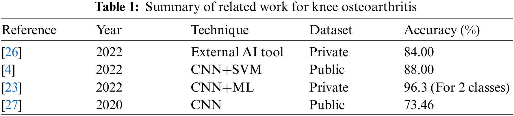
A method was created by combining the Xception model, ImageNet, and a dataset containing X-ray images from TKA patients. An ML model was then created based on this information. Another ML model was also developed using a random forest classifier built on a different system and used a dataset containing TKA patient clinical parameters. To understand the model’s predictions, class activation maps were employed. The ML model for the image-based loosening achieved a precision of 0.92 while having a recall of 0.96, with a 96.3% accuracy for classification. However, incorporating a clinical information-based framework did not enhance accuracy, as it obtained a precision of 0.71 and a recall of 0.20 [23]. Finally, Chan et al. in [24] developed an efficient DL model for evaluating malignancies in knee bones. A mix of unsupervised and supervised algorithms was utilized to recognize important patterns in recognition of common and atypical bones and bone cancers. The results demonstrated that the model’s efficiency surpasses that of other notable models.

In [25], the authors examined and compared the acoustic emissions (AE) and kinematic instability (KI) of osteoarthritic (OA) knee joints to radiography findings. Sixty-six women and 43 men between the ages of 44 and 67 were recruited. On radiographs, the narrowing of the joint space was inspected. Moreover, osteophytes, as well as Kellgren–Lawrence (KL) grade, were also examined. Fifty-four participants in the group were identified with radiographic OA-based radiography, whereas 55 subjects comprised the control group. AE and KI were measured using a custom prototype framework and compared to radiography results using area-under-curve (AUC) and independent T-test. Leave-one-out cross-validation was utilized to develop predictive logistic regression models. In females, KI, BMI, and age, representing the constancy of AE patterns throughout certain tasks, differed significantly between the OA and control groups (p = 0.001–0.036). The chosen AE signals, KI, age, and BMI were used to develop a prediction model for radiographic OA with an AUC of 90.3%, statistically superior to the reference model based on age and BMI, which had an AUC of 84.2%. The predictive model did not enhance the reference model for guys. AE and KI give complementary information for the radiographic diagnosis of knee osteoarthritis in females. A summary is given in Table 1.

3  Proposed Methodology

The framework to achieve the results starts by implementing the preprocessing technique. Images histograms are equalized, and the resultant dataset is fed to two pre-trained networks that are Efficientnetb0 and Densenet201. Using a transfer learning strategy, models are trained to modified networks. Moreover, deep features are extracted by applying both trained networks to obtain feature vectors from Efficientnetb0 and Densenet201 named Veff and Vden. Furthermore, extracted features are combined using the feature fusion technique. Also, the best features are selected by implementing the whale optimization technique. Selected features are further sliced and given as input to classifiers to obtain results. Fig. 3 shows the steps taken in the proposed methodology.

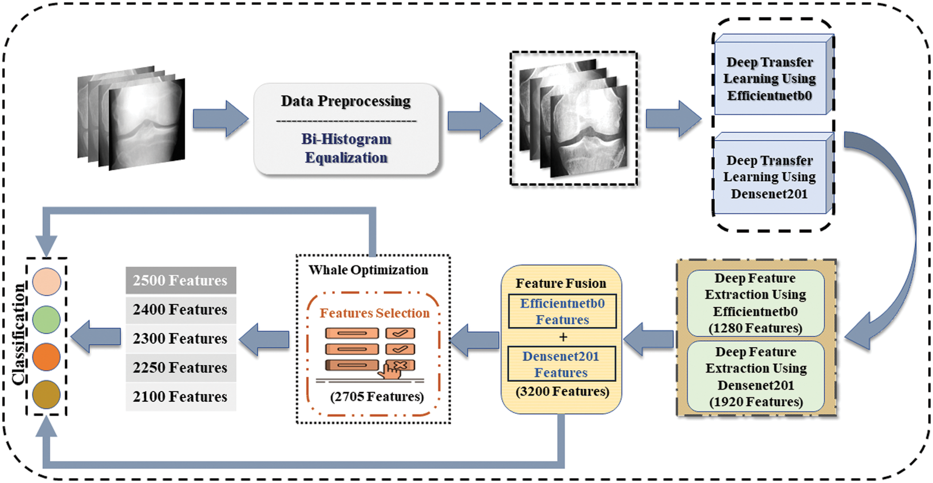
Figure 3: Proposed methodology for osteoarthritis classification using deep learning

3.1 Dataset

In this study, the used knee joints dataset is available to the public [28], which comprises 7828 images. Furthermore, the dataset is divided into two sets, i.e., training and testing set that includes seventy percent for training, whereas thirty percent is segregated for testing purposes. The dataset is in two channels; thus, it is changed to three channels since deep learning models only accept images with three channels. The dataset contains four classes named 0, 1, 2, and 3. Class 0 represents healthy knee X-ray images, class 1 shows Doubtful knee joint narrowing, class 2 depicts moderate disorder, and class 3 shows severe knee joint disorder. Class 0 contains 3085 images, class 1 contains 1416 images, and class 2 have 2062 image, whereas the last class, i.e., class 3, includes 1265 images of knee joints.

3.2 Preprocessing

Preprocessing is an important step to enhance the dataset, which may impact highly on required results. Brightness Preserving Histogram Equalization (BPHE) technique is used to improve the quality of images.

Brightness-preserving histogram equalization is a contrast enhancement method in image processing [29]. It aims to improve the visual quality of an image by adjusting the distribution of intensity levels so that the image has a more uniform histogram. Unlike traditional histogram equalization methods, preserving bi-histogram equalization considers an input image’s bright and dark regions. It adjusts the histograms of each independently to preserve details in both bright and dark regions while enhancing overall contrast. This technique is particularly useful in medical imaging and other applications where preserving the detail in both bright and dark regions is important. To achieve brightness preservation, the input image is divided into two parts. Lower bound set (Slower) consists of images with low-contrast pixels while the upper bound set (Shigher) consists of high-contrast pixels. i.e.,:

SInp=(Slower)⋃(Shigher)(1)

(Slower)={S(j,k)|S(j,k)≤Smean,∀S(j,k)∈S(2)

(Shigher)={S(j,k)|S(j,k)>Smean,∀S(j,k)∈S(3)

The probabilistic density function for both (Slower) and (Shigher) parts are as follows:

(Qprob)l(Sp)=OlpOl,wherep=0,1,2,…,N(4)

(Qprob)h(Sp)=OhpOh,wherep=N+1,N+2,…,N−K(5)

Here, Olp and Ohp are the number of Sp in (Slower) and (Shigher) respectively. Similarly, cumulative density functions for both parts are given below:

Dl(Sp)=∑k=0p⁡(Qprob)l(Sk)(6)

Dh(Sp)=∑k=N+1p⁡(Qprob)h(Sk)(7)

The transform function for the lower and upper parts are as follows:

FunL(Sp)=S0(SN−S0)Dl(Sp)(8)

Funh(Sp)=S0(SN−S0)Dh(Sp)(9)

The final image having equalized histogram with preserved brightness can be obtained by combining both equations, that is:

SBPHE=FunL(Sp)∪Funh(Sp)(10)

Here, SBPHE is the Brightness Preserved Histogram Equalized image. Sample images from the preprocessed dataset are shown in Fig. 4.

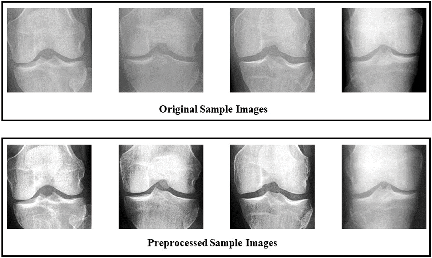
Figure 4: Comparison between original and preprocessed dataset using sample images

3.3 Convolutional Neural Network

CNNs are widely used in the medical image processing domain. A network is called CNN if a minimum of one layer performs a convolution operation. In a convolution operation, a filter of a specific size having multiple parameters is run through an input image in the sliding windows method. The resultant image is passed to the next layer for further operations. Mathematically it is represented as:

Imgout{rout×cout}=(imginp∗kop)(11)

where, Imgout is the output matrix having rout and cout rows and columns, respectively. Moreover, kop is the kernel used for convolution operation. Furthermore, the rectified linear unit function is applied to obtain the negative feature’s value as zero, which can be represented in the equation below:

ReLu=Max(0,a),a∈Imgout(12)

Also, the pooling operation is performed to minimize the data to improve the time cost. Then, two different functions are performed either maximum or average values of the specific area are extracted and replaced with the central input value. Finally, a fully connected layer flattens the features and extracts a one-dimensional vector. Mathematically it is denoted as:

(Vecfeat)0out=Imgout{rout×cout}(13)

(Vecfeat)iin=(Vecfeat)i−1out∗Imgi+ci(14)

(Vecfeat)iout=Δi((Vecfeat)iin)(15)

Here, (Vecfeat)iout is flattened vector, Δ is activation function, and i is layer number. The softMax layer is inserted to obtain the probability of the feature for the class that is shown as:

SOFTMAX((Vecfeat)iout)=exp((Vecfeat)iout)∑k(Vecfeat)kout(16)

3.4 Feature Extraction

Features extraction is the most important step in DL. Two pre-trained models, i.e., Efficientnetb0 [30] and Densenet201 [31], are trained using the transfer learning technique. The dataset is divided into training and testing parts, with 70% training and 30% testing images. Transfer learning (TL) principles were selected for the training of refined models. Since the pre-trained neural networks are trained on a subset of classes (i.e., the ImageNet dataset), while the medical image classification task is the objective in our situation, the pre-trained neural networks are not applicable. Therefore, we must train the network using a carefully selected knee orthosis dataset. In the case of the Efficientnetb0 model, the layers classification, ‘softmax,’ and ‘efficientnet-b0|model|head|dense|MatMul’ are replaced with ‘new_ classification,’ ‘new_softmax,’ and ‘new_efficientnet-b0|model|head|dense|MatMul’ layers. The size of the vector obtained through ‘new_softmax,’ and ‘new classification’ layers is [1 × 1 × 4], as the dataset used in this study contains four classes while the model is pretrained with one thousand classes. In the instance of Densenet201, the layers ‘fc1000,’ fc1000_softmax,’ and ClassificationLayer_fc1000’ are changed with ‘new_ classification,’ '“new_softmax” and ‘new_ ClassificationLayer_fc1000’ layers. The vector obtained from the new layers have the size of [1 × 1 × 4], as the number of classes in the dataset is 4. while the pretrained network is trained using thousand number of classes. The hyperparameters are initialized with the following values: the mini-batch size of 8, the initial learning rate of 0.01, epochs of 150, the dropout factor of 0.4 and the optimizer used is Adam. TL is then used to train the newly refined models. Moreover, features are extracted from both networks. Veff and Vden are the feature vectors having 1280 features and 1920 features respectively. Veff is obtained from Efficientnetb0 through the global average pooling layer named “efficientnetb0|model|head|global_average_pooling2d|GlobAvgPool” whereas Vden is extracted through Densenet201 from the average pooling layer named “avg_pool”.

3.5 Feature Fusion

As mentioned above, two feature vectors Veff and Vden are extracted from both networks used in this methodology, it is necessary to combine both vectors to enlarge the feature vector having more information. Correlation extended serial approach is used to fuse both of the vectors, which can mathematically be shown as:

Crelation=∑(Ri−R¯)(Xj−X¯)∑(Ri−R¯)2∑(Xj−X¯2)(17)

In above equation, Ri and Xj are the features from Veff and Vden whereas R¯ and X¯ are mean value of Veff and Vden. Based on this method, the features with a +ve correlation (+1) are selected into a new vector labeled Vc3 and the features with a correlation value of 0 or −1 are added to Vc4. Then, the mean value of Vc4 is determined by:

CrelationT={Vecupd,Vc4≥0Ignore_feat,Vc4<0(18)

By using the mathematical formulation below, both vectors are fused.

VecFinal=(VecupdVc3)(19)

The final fused vector VecFinal has 3200 features.

3.6 Feature Optimization

Whale optimization (WOA) is used in this work to reduce the dimension of feature vectors, which helps avoid the curse of dimensionality. Fused vector VecFinal is then fed to WOA to extract the selected feature vector.

The whale feature selection technique, which is a nature-based metaheuristic algorithm designed by Mirjalili, is used to acquire the most important features from a large set of features [32]. Whales search and prey on food in a unique manner which researchers adopt to achieve the best feature selection. In the first step, it generates k humpback whales and disperses them at random across the search space. After assessing each whale’s position, the best humpback whales are chosen. The other whales will try to get closer to the top whale. Humpback whales begin to adopt a bubble-net tactic in the second phase of the attack. There are two strategies: spiral positioning for bubble-net attacks and shrinking encircling. This step is actually identical to the exploitation phase, in which each whale suggests a subset of features. The classifier’s accuracy on the testing set is then utilised to evaluate these feature subsets. In the third stage, known as the exploration phase, humpback whales hunt for prey at random based on their position in relation to one another.

Firstly, the whales randomly search for their prey. Then, when the prey is located, it is encircled by adopting the spiral position updating technique. Mathematically these steps are denoted by:

D=|EZ∗(j)−Z(j)|(20)

Z(j+1)=Z∗(i)−CD(21)

Here, j is explained as the most recent iteration number while Z∗(j) is the whale which is in the best position with respect to the food source. Furthermore, Z(j) is current whale position. C and E are the coefficients that are described as:

C=2ct1−c(22)

E=2t2(23)

where, t1 and t2 are two casual parameters having values of zero and one respectively. Moreover, c is the convergent factor calculated as:

c=2−2JJMax(24)

where, JMax is the total number of iterations, while J is the current iteration. As mentioned above, whales use encircled positional updating method to achieve minimization of distance to the food source; hence, the mathematical formulation for the method is given as:

Z(j+1)=Z∗(j)−Fqeclcos⁡(2πl)(25)

Above, Fq is the distance between the source of food and the current whale. l is the unintended number ranging from zero to one. As the whale uses the spiral updating method, it must contract the circle around the food source to minimize the distance. The probability for this method is calculated as:

Z(j+1)={Z∗(i)−CDprob<PbZ∗(j)−Fqeclcos⁡(2πl)prob≥Pb(26)

In the initial stage, whales have to go randomly searching for food sources. Hence, each whale must update its position within the area yet at some random point to detect the food source. Therefore, the fitness is checked for each iteration, and Fine- K Nearest Neighbor (F-KNN) classifier is employed as a fitness function. Mathematically, the random point is denoted by equations as follows:

F=EZrand−Z(j)(27)

Z(j+1)=Zrand−CF(28)

Here, Z(j) is the position vector for a whale that is chosen causally. An agent called a seeking agent is used to force the whales for position updating according to the current whale, which may help in finding a new source.

4  Results and Analysis

This study is implemented on MATLAB-2021A—a windows-based machine with a GTX 950M GPU.

4.1 Numerical Results

This section covers the results achieved using the proposed methodology. Results are given in the tabular form, confusion matrix, and graphical form. Table 2 represents the results achieved using different classifiers, according to the table below fine-tuned Linear Support Vector Machine (LSVM) obtained the highest accuracy of 90.1 percent. In LSVM, one vs. all strategy is adopted to fine-tune the algorithm. Also, fine-tuned LSVM obtained a Precision value of 0.88, a Recall value of 0.89, and an F1 Score of 0.88. Fig. 5 illustrates the confusion matrix of fine-tuned LSVM classification. LSVM without tuning achieved better time cost than all other classifiers and attained 89.9 percent accuracy. Different Neural Networks are also used to classify, and results are accessed in the table below.

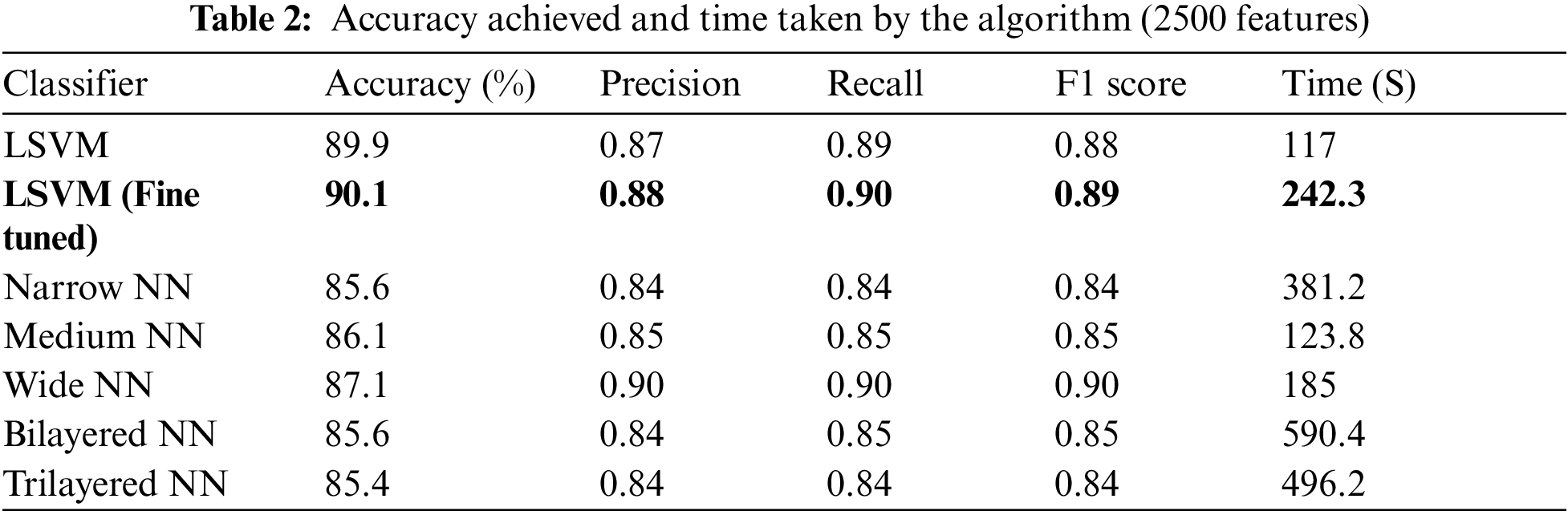
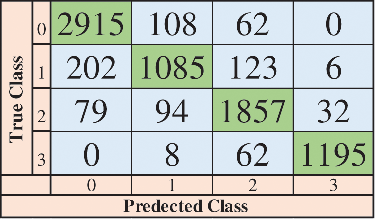
Figure 5: Confusion matrix of LSVM (fine-tuned)

Fig. 6 shows the time cost of classifiers used in the proposed methodology, while Fig. 7 represents the comparison of accuracy obtained by different classifiers. Fig. 8 compares time cost and accuracy obtained by different classifiers. Features are selected using the whale optimization technique and accessed the results. Also, selected features are further sliced into minimal feature sets. Furthermore, each sliced feature set is fed to the classification algorithm and achieves accuracy. Table 3 represents the accuracy and time cost attained by each classifier.

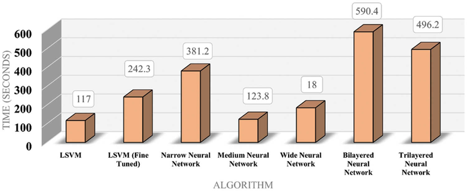
Figure 6: Time bar chart for classifiers

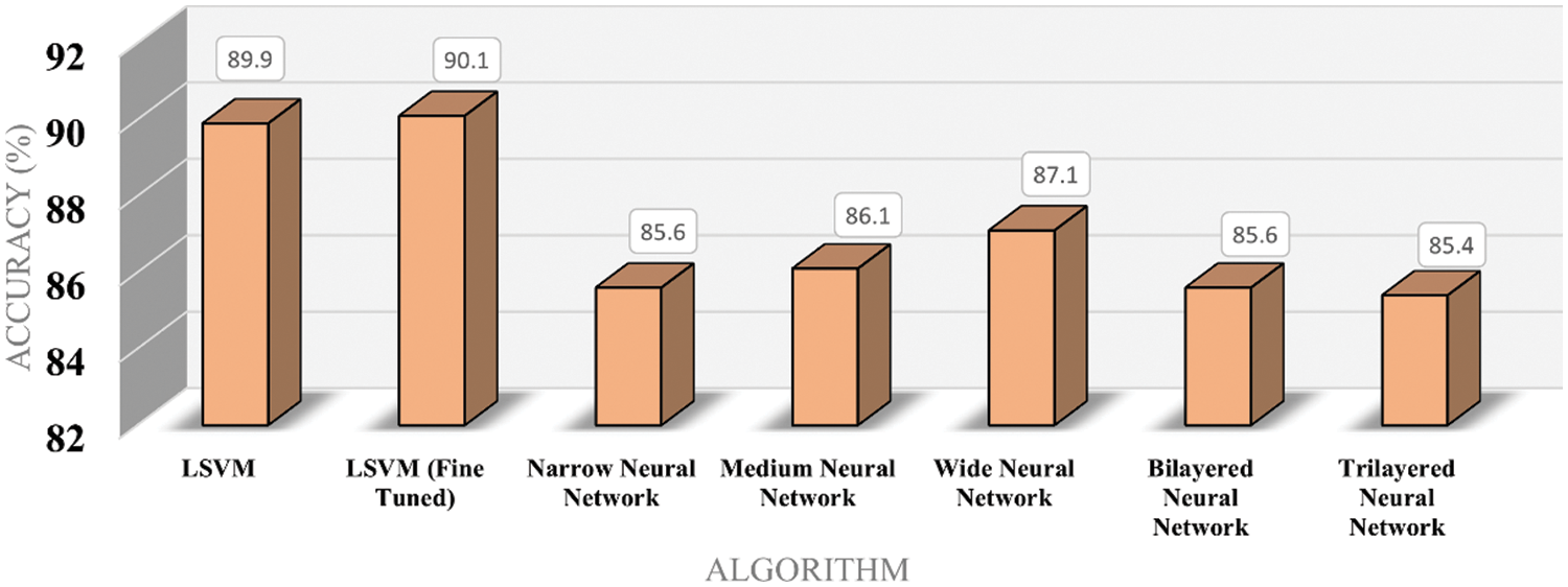
Figure 7: Accuracy bar chart for classifiers

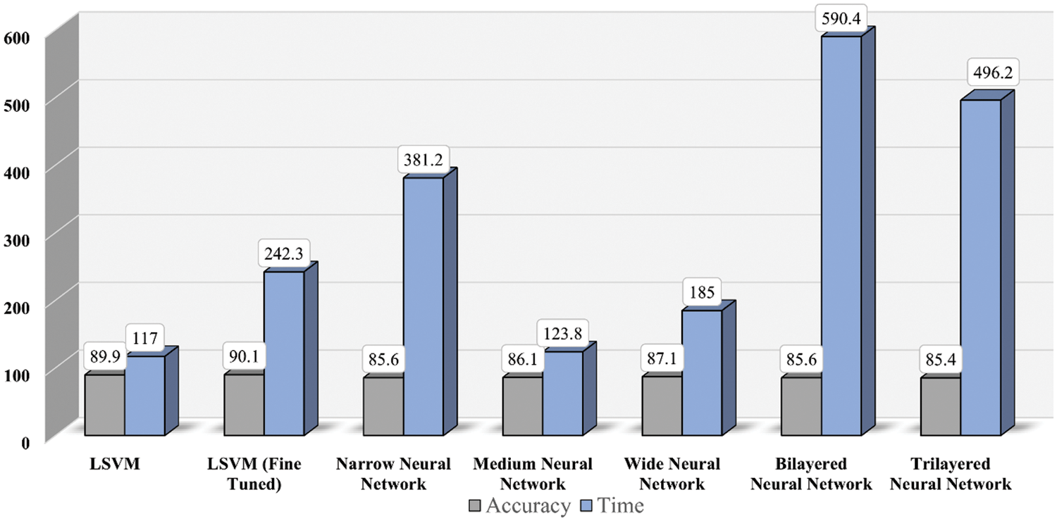
Figure 8: Time and accuracy comparison for classifiers

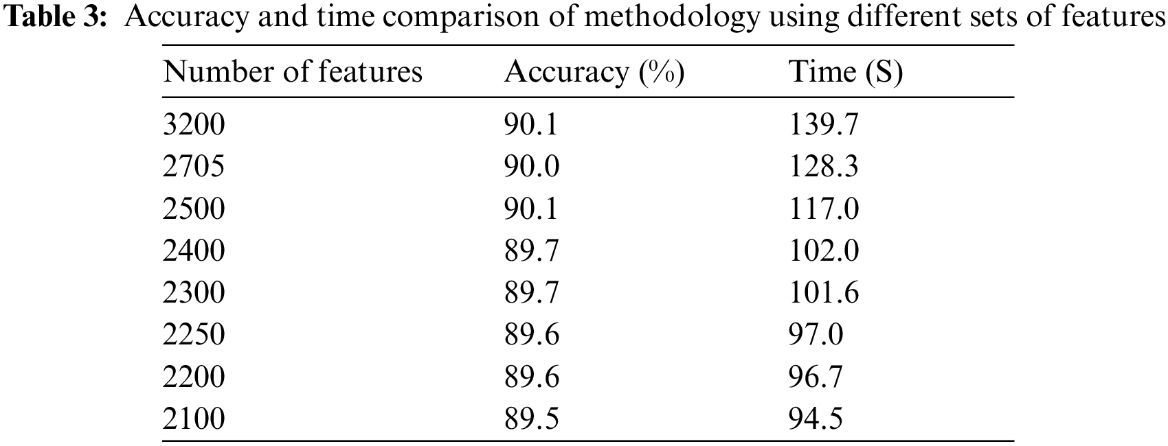
It is accessed in the graph shown in Fig. 9 that accuracy is enhanced as the number of features is increased. Trendline depicts the gradual increase in the accuracy on each step of the features increment. Similarly, the graph in Fig. 10 shows that the time cost also expands as the number of features increases. Analytics of both graphs represents that any increment in features after 2500 features does not affect accuracy while time cost increases rapidly. Fig. 11 combines the graphs and shows accuracy vs. time concerning the number of features.

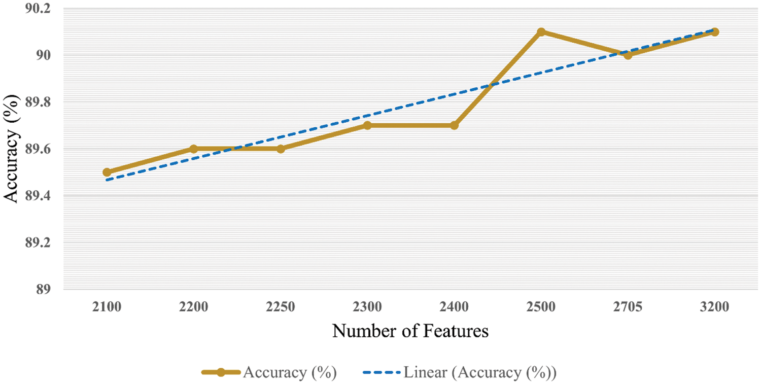
Figure 9: Accuracy with respect to number of features

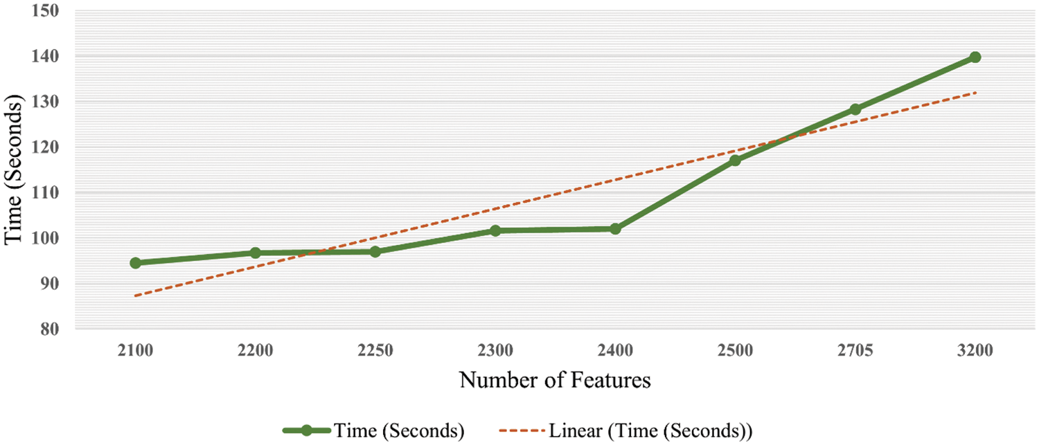
Figure 10: Time graph with respect to number of features

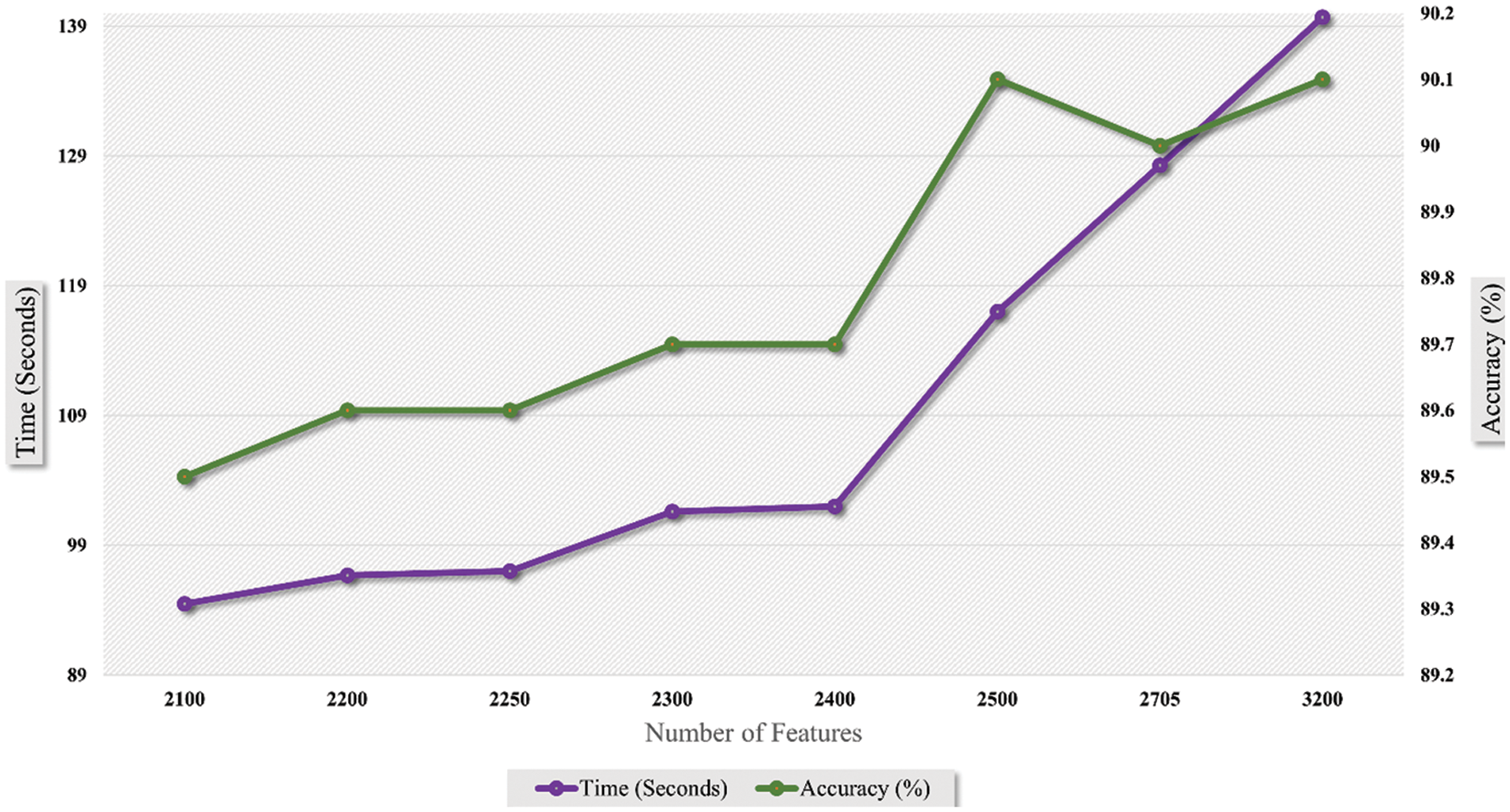
Figure 11: Time vs. accuracy graph with respect to number of features

4.2 Explainable Artificial Intelligence

Explainable artificial intelligence (XAI) [33] refers to intelligent systems that can give researchers clear and trustworthy descriptions of their decision-making process. XAI is crucial because it enables humans to comprehend why an AI system makes particular predictions, judgments, or suggestions and to spot any biases or flaws in its thinking. This can boost confidence in AI systems and guarantee that they are employed following human values and ethical standards.

Explainable artificial intelligence (XAI) uses occlusion [34] to determine each individual’s contribution to a model’s forecast. The method includes masking or obstructing portions of an input and evaluating how the model’s output varies. By reiterating this procedure for various input sections, it is feasible to determine which elements are most crucial for the model’s prediction and which are driving the model’s behavior. Frequently, occlusion is used to construct saliency maps or heat maps, as represented in Fig. 12, which are visual representations of the importance of each feature to the model’s prediction for each class sample of the dataset. This can help comprehend a model’s decisions and identify any biases or errors in its predictions.

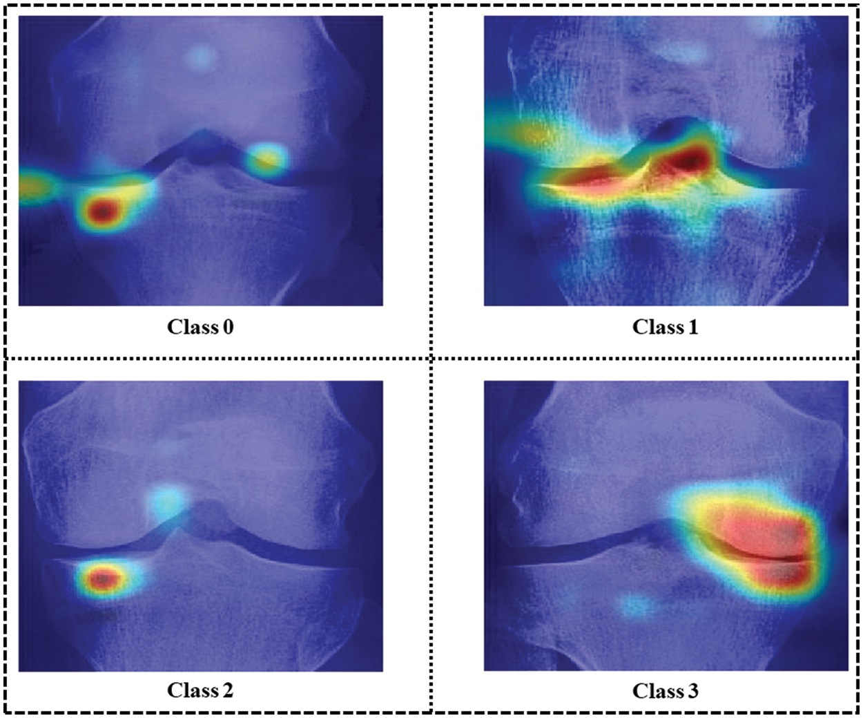
Figure 12: Occlusion for all four classes of sample images

Mesh plots in Fig. 13 depict the density of important features inside the input image area. Test images are taken from each dataset class and predicted by the trained network. A heatmap for the area with dense important features is extracted by applying the occlusion technique. As shown in Fig. 13 it is clear that class 0 and class 2 sample images are not classified correctly, while class 1 and class 3 sample images are classified correctly. This is because the dense area for the class 0 sample image is classified as class 2 whereas the class 0 sample image belongs to the normal class. Similarly, class 2 sample image features are extracted from the image area where knee disorder is not impacted. On the other hand, class 1 and class 3 are correctly classified, and the dense feature area is correctly highlighted.

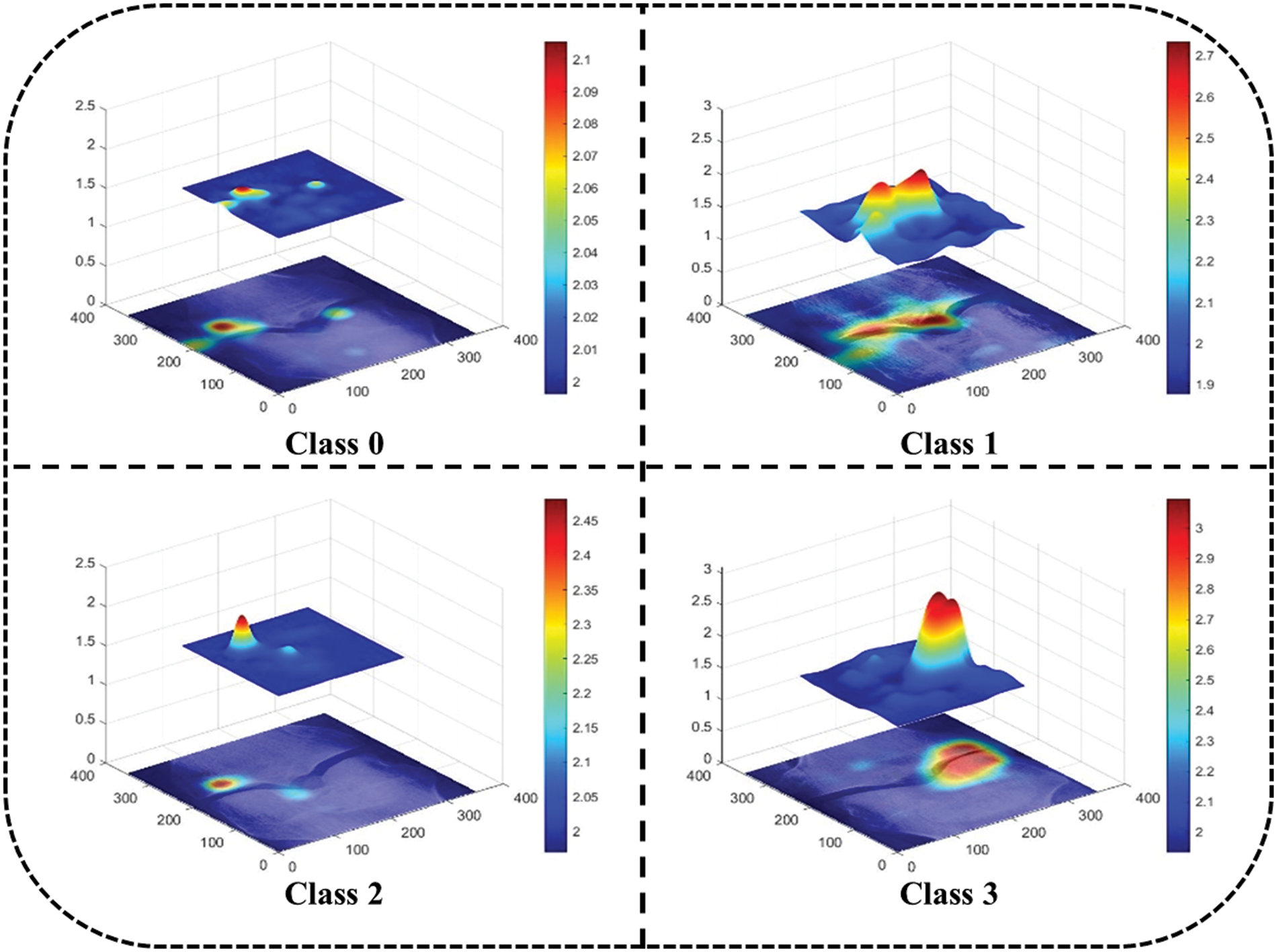
Figure 13: Map plot for occlusion for all classes

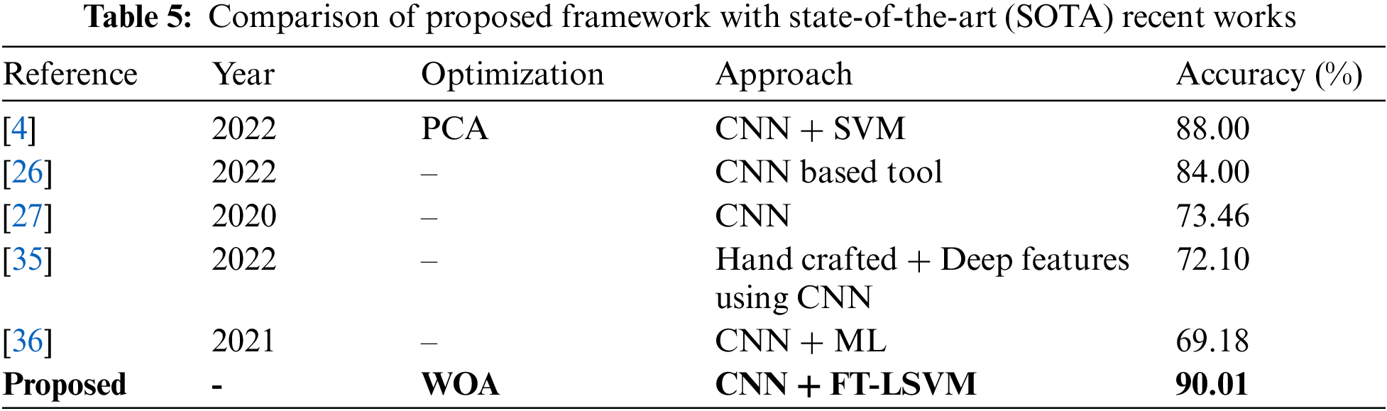
In the last, we compare the proposed method’s accuracy with several other neural nets, as given in Table 4. All models are tested on the selected datasets as used for the proposed framework. This table shows that the defined model’s accuracy is 90.1%, 85.3%, 82.9%, 84.76%, 86.22%, and 87.32%, respectively. After the proposed model, the accuracy of the ResNet101 deep model is better. In addition, a confidence interval-based analysis is also given in Fig. 14. This figure shows that the margin of error after 100 times iterations is 88.95 ± 1.594 (±1.79%). This means that the 1.79% error is noted. Hence, based on this, it can be concluded that the proposed framework’s accuracy remains consistent. A comparison with the recent state-of-the-art methods is also performed, as noted in Table 5. This table shows that the proposed method accuracy is compared with several state-of-the-art (SOTA) techniques. In this table, an efficient deep mixture approach is introduced by Ahmed et al. [4] and obtained a classification accuracy of 88%. In [26], the authors presented an artificial intelligence based technique and obtained 84% accuracy for the classification. The other methods, such as [27,35] and [36], the authors obtained accuracies of 73.46%, 72.10%, and 69.18%. Therefore, the proposed approach achieves an accuracy of 90.1%, which is 2% improved than the recent methods.

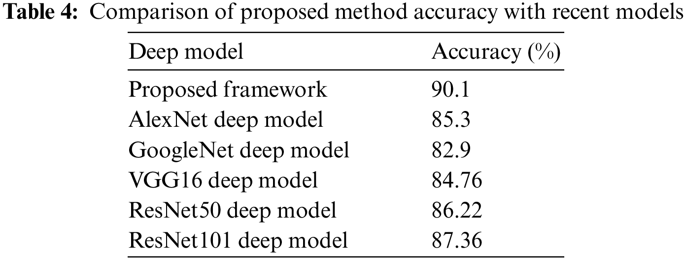
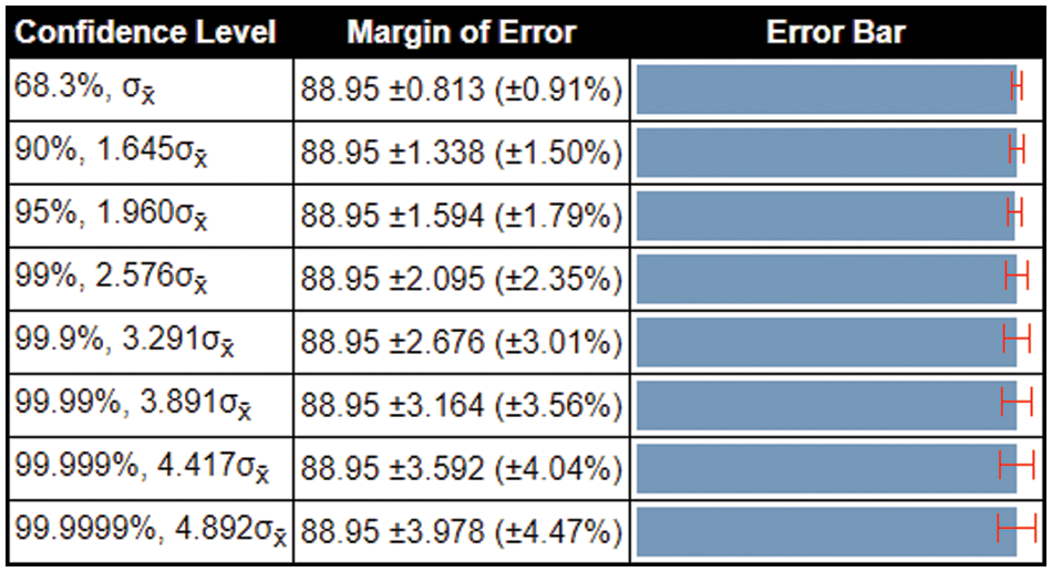
Figure 14: Margin of error-based analysis of the proposed framework accuracy

5  Conclusion

A new framework is proposed in this work for the classification of knee osteoarthritis. Two pre-trained deep learning models have been utilized for deep feature extraction, and later, fusion is performed using a canonical correlation approach. By employing this approach, information from both sources has been combined for better accuracy performance. Moreover, the dimensionality reduction technique is applied to acquire the best features that are finally classified using machine learning classifiers. In conclusion, the proposed approach obtained better multi-class classification accuracy of 90.1% compared to previous research. Also, it is accessed through this study that features slicing may positively impact increasing accuracy while keeping time cost as low as possible. The work also elaborates that Efficientnetb0 and Densenet201 obtained better results if the extracted features were combined using a correlation extended serial approach. Multiple sets of features are given as input to the system and accessed that time and accuracy have inversely proportional relation for the number of features. Furthermore, the prediction of the system is explained by occlusions which highlight the dense feature areas of images. The key limitation of this work is the extraction of some redundant information that misleads the classification performance and increases the computational time. In the future, this issue can be resolved by employing the customized CNN model with residual block and Bayesian optimization.

Funding Statement: This work was supported by “Human Resources Program in Energy Technology” of the Korea Institute of Energy Technology Evaluation and Planning (KETEP), granted financial resources from the Ministry of Trade, Industry & Energy, Republic of Korea. (No. 20204010600090).

Conflicts of Interest: The authors declare that they have no conflicts of interest to report regarding the present study.

References

1. W. Laupattarakasem, M. Laopaiboon, P. Laupattarakasem and C. Sumananont, “Arthroscopic debridement for knee osteoarthritis,” Cochrane Database of Systematic Reviews, vol. 6, no. 1, pp. 1–16, 2008. [Google Scholar]

2. J. C. Mora, R. Przkora and Y. Cruz-Almeida, “Knee osteoarthritis: Pathophysiology and current treatment modalities,” Journal of Pain Research, vol. 6, no. 2, pp. 2189–2196, 2018. [Google Scholar]

3. K. Maiese, “Picking a bone with WISP1 (CCN4New strategies against degenerative joint disease,” Journal of Translational Science, vol. 1, no. 3, pp. 83, 2016. [Google Scholar] [PubMed]

4. S. M. Ahmed and R. J. Mstafa, “Identifying severity grading of knee osteoarthritis from x-ray images using an efficient mixture of deep learning and machine learning models,” Diagnostics, vol. 12, no. 12, pp. 2939, 2022. [Google Scholar] [PubMed]

5. F. K. Ciliberti, L. Guerrini, A. E. Gunnarsson and M. Recenti, “CT-and MRI-based 3D reconstruction of knee joint to assess cartilage and bone,” Diagnostics, vol. 12, no. 5, pp. 279, 2022. [Google Scholar] [PubMed]

6. R. Smith, P. Egger, D. Coggon, M. Cawley and C. Cooper, “Radiological assessment of osteoarthritis of the hip joint and acetabular dysplasia in osteoarthritis,” Annals of the Rheumatic Diseases, vol. 16, no. 4, pp. 494–502, 1957. [Google Scholar]

7. M. D. Kohn, A. A. Sassoon and N. D. Fernando, “Classifications in brief: Kellgren-lawrence classification of osteoarthritis,” Clinical Orthopaedics and Related Research®, vol. 474, no. 5, pp. 1886–1893, 2016. [Google Scholar] [PubMed]

8. N. Bayramoglu, M. T. Nieminen and S. Saarakkala, “A lightweight cnn and joint shape-joint space () descriptor for radiological osteoarthritis detection,” in Medical Image Understanding and Analysis: 24th Annual Conf., MIUA 2020, Oxford, UK, pp. 331–345, 2020. [Google Scholar]

9. D. H. Kim, S. C. Kim, J. S. Yoon and Y. S. Lee, “Are there harmful effects of preoperative mild lateral or patellofemoral degeneration on the outcomes of open wedge high tibial osteotomy for medial compartmental osteoarthritis?,” Orthopaedic Journal of Sports Medicine, vol. 8, no. 6, pp. 2325967120927481, 2020. [Google Scholar] [PubMed]

10. L. Anifah, I. K. E. Purnama, M. Hariadi and M. H. Purnomo, “Osteoarthritis classification using self organizing map based on gabor kernel and contrast-limited adaptive histogram equalization,” The Open Biomedical Engineering Journal, vol. 7, no. 12, pp. 18, 2013. [Google Scholar] [PubMed]

11. R. T. Wahyuningrum, L. Anifah, I. K. E. Purnama and M. H. Purnomo, “A novel hybrid of S2DPCA and SVM for knee osteoarthritis classification,” in 2016 IEEE Int. Conf. on Computational Intelligence and Virtual Environments for Measurement Systems and Applications (CIVEMSA), NY, USA, pp. 1–5, 2016. [Google Scholar]

12. M. Varma, “Automated abnormality detection in lower extremity radiographs using deep learning,” Nature Machine Intelligence, vol. 1, no. 12, pp. 578–583, 2019. [Google Scholar]

13. S. Malik, T. Akram, M. Awais, M. Hadjouni and H. Elmannai, “An improved skin lesion boundary estimation for enhanced-intensity images using hybrid metaheuristics,” Diagnostics, vol. 13, no. 5, pp. 1285, 2023. [Google Scholar] [PubMed]

14. K. Jabeen, J. Balili, M. Alhaisoni, N. A. Almujally and H. Alrashidi, “BC2NetRF: Breast cancer classification from mammogram images using enhanced deep learning features and equilibrium-jaya controlled regula falsi-based features selection,” Diagnostics, vol. 13, no. 2, pp. 1238, 2023. [Google Scholar] [PubMed]

15. A. Hamza, A. Al Hejaili, K. A. Shaban and S. Alsubai, “D2BOF-COVIDNet: A framework of deep bayesian optimization and fusion-assisted optimal deep features for COVID-19 classification using chest x-ray and MRI scans,” Diagnostics, vol. 13, no. 11, pp. 101, 2023. [Google Scholar]

16. F. Jahangir, A. Alqahtani, S. Alsubai and M. Sha, “A fusion-assisted multi-stream deep learning and ESO-controlled newton-raphson-based feature selection approach for human gait recognition,” Sensors, vol. 23, no. 6, pp. 2754, 2023. [Google Scholar] [PubMed]

17. M. Ajmal, T. Akram, A. Alqahtani, M. Alhaisoni and A. Armghan, “BF2SkNet: Best deep learning features fusion-assisted framework for multiclass skin lesion classification,” Neural Computing and Applications, vol. 4, no. 7, pp. 1–17, 2022. [Google Scholar]

18. M. A. Khan, A. Khan, M. Alhaisoni, A. Alqahtani and S. Alsubai, “Multimodal brain tumor detection and classification using deep saliency map and improved dragonfly optimization algorithm,” International Journal of Imaging Systems and Technology, vol. 33, no. 12, pp. 572–587, 2023. [Google Scholar]

19. J. H. Kellgren and J. Lawrence, “Radiological assessment of osteo-arthrosis,” Annals of the Rheumatic Diseases, vol. 16, no. 4, pp. 494–502, 1957. [Google Scholar] [PubMed]

20. X. Zhang, D. Lin, J. Jiang and Z. Guo, “Preliminary study on grading diagnosis of early knee osteoarthritis by shear wave elastography,” Contrast Media & Molecular Imaging, vol. 2022, no. 5, pp. 5–6, 2022. [Google Scholar]

21. D. P. Yadav, A. Sharma, S. Athithan, A. Bhola, B. Sharma et al., “Hybrid SFNet model for bone fracture detection and classification using ML/DL,” Sensors, vol. 22, no. 15, pp. 5823, 2022. [Google Scholar] [PubMed]

22. Q. Zhang, J. Wang, H. Zhou and C. Xia, “Automatic segmentation of knee meniscus based on magnetic resonance images,” in Proc. of 2021 Chinese Intelligent Systems Conf., Bejing, China, pp. 153–162, 2021. [Google Scholar]

23. L. C. M. Lau, “A novel image-based machine learning model with superior accuracy and predictability for knee arthroplasty loosening detection and clinical decision making,” Journal of Orthopaedic Translation, vol. 36, no. 4, pp. 177–183, 2022. [Google Scholar] [PubMed]

24. L. Chan, H. Li, P. Chan and C. Wen, “A machine learning-based approach to decipher multi-etiology of knee osteoarthritis onset and deterioration,” Osteoarthritis and Cartilage Open, vol. 3, no. 1, pp. 100135, 2021. [Google Scholar] [PubMed]

25. M. T. Nevalainen, “Acoustic emissions and kinematic instability of the osteoarthritic knee joint: Comparison with radiographic findings,” Scientific Reports, vol. 11, no. 1, pp. 19558, 2021. [Google Scholar] [PubMed]

26. M. W. Brejnebøl, P. Hansen, J. U. Nybing and R. Bachmann, “External validation of an artificial intelligence tool for radiographic knee osteoarthritis severity classification,” European Journal of Radiology, vol. 150, no. 6, pp. 110249, 2022. [Google Scholar]

27. A. Tiulpin and S. Saarakkala, “Automatic grading of individual knee osteoarthritis features in plain radiographs using deep convolutional neural networks,” Diagnostics, vol. 10, no. 5, pp. 932, 2020. [Google Scholar] [PubMed]

28. Kaggel, “Kaggle dataset,” 2023. [Online]. Available: https://www.kaggle.com/datasets/maangelikaferrer/knee-osteoarthritis-dataset [Google Scholar]

29. Y. T. Kim, “Contrast enhancement using brightness preserving bi-histogram equalization,” IEEE Transactions on Consumer Electronics, vol. 43, no. 6, pp. 1–8, 1997. [Google Scholar]

30. M. Tan and Q. Le, “Efficientnet: Rethinking model scaling for convolutional neural networks,” in Int. Conf. on Machine Learning, NY, USA, pp. 6105–6114, 2019. [Google Scholar]

31. Y. Zhu and S. Newsam, “Densenet for dense flow,” in 2017 IEEE Int. Conf. on Image Processing (ICIP), NY, USA, pp. 790–794, 2017. [Google Scholar]

32. S. Mirjalili and A. Lewis, “The whale optimization algorithm,” Advances in Engineering Software, vol. 95, no. 12, pp. 51–67, 2016. [Google Scholar]

33. D. Gunning, M. Stefik, J. Choi, T. Miller and S. Stumpf, “XAI—Explainable artificial intelligence,” Science Robotics, vol. 4, no. 7, pp. eaay7120, 2019. [Google Scholar] [PubMed]

34. R. Machlev, M. Perl, J. Belikov, K. Y. Levy and Y. Levron, “Measuring explainability and trustworthiness of power quality disturbances classifiers using XAI—explainable artificial intelligence,” IEEE Transactions on Industrial Informatics, vol. 18, no. 2, pp. 5127–5137, 2021. [Google Scholar]

35. M. Y. Sikkandar, S. S. Begum, A. A. Alkathiry and M. D. Manzar, “Automatic detection and classification of human knee osteoarthritis using convolutional neural networks,” Computers, Materials & Continua, vol. 70, no. 2, pp. 4279–4291, 2022. [Google Scholar]

36. Y. Wang, X. Wang, T. Gao, L. Du and W. Liu, “An automatic knee osteoarthritis diagnosis method based on deep learning: Data from the osteoarthritis initiative,” Journal of Healthcare Engineering, vol. 2021, no. 2, pp. 1–10, 2021. [Google Scholar]