A Graph Neural Network Recommendation Based on Long- and Short-Term Preference

1  Introduction

Internet technology has increased the information available to users, resulting in an information overload problem. It is essential to recommend the content that users are interested in from the vast amount of information available. In this context, the concept of recommendation systems (RS) was proposed [1]. RS model users’ interest preferences based on their personal information and browsing history and then make personalized recommendations for users based on their interest preferences. RS is currently attracting extensive research in academia and industry [2,3].

In real-world scenarios, the interaction data in RS is essentially a large graph structure where most objects are connected explicitly or implicitly. This inherent data characteristic makes it necessary to consider complex inter-object relationships when making recommendations. Therefore, with the research and development of Graph Neural Network (GNN), more and more researchers are using GNN for RS to extract node information about the associations between users and items. Berg et al. [4] used a GNN to fill in the missing rating information in the interaction graph. Ying et al. [5] combined a random walk and a GNN to generate node embeddings that contain the nodes’ graph structure and feature information. Zhang et al. [6] proposed using multi-connected graph convolutional encoders to learn node representations. Wang et al. [7] introduced the idea of residuals into a GNN to multiple aggregate layers of neighbor representations into the final node representation.

Although GNN-based RS excels in feature extraction, current GNN-based RS usually constructs a user-item interaction graph using all items that users have interacted with in the past [8,9], and then generates long-term preference representations by performing neighborhood aggregation on the graph. In addition to relatively stable long-term preferences, user preferences are inherently dynamic, and over time and with some trend guidance, they may also generate some short-term preferences. Further, short-term preferences are more likely to lead to user-item interactions. Therefore, on top of the long-term preference representation captured by the user-item interaction graph, combining the long-term preference representation with the short-term preference representation will yield better recommendation results. At the same time, due to the data sparsity caused by the huge amount of data, the item features obtained by constructing the user-item interaction graph using IDs alone may not be sufficient. Therefore, based on the features of item nodes captured by GNN, combining other attribute information of items can further capture more adequate item features.

In summary, we propose a GNN recommendation model based on long- and short-term preference (LSGNN), with the following main contributions:

1)   Design a new methodological framework. This recommendation framework fuses long-term preference features and short-term preference features. It combines item title and description information to achieve predictive recommendations based on the fused features.

2)   Design a new short-term preference feature extraction model. First, semantic information is extracted using Bidirectional Encoder Representation from Transformers (BERT). Then, the information of recent interaction data is captured by Bi-directional Gated Recurrent Unit (Bi-GRU) to empower the model to analyze recent preference features. Finally, the recent interaction features are given different attention weights by the attention mechanism, which allows the model to extract more helpful preference features.

3)   Design a new item text feature extraction model. First, semantic information is extracted using BERT. Then, the hidden word representations in the item words are captured by a Convolutional Neural Network (CNN). Finally, the final text representation is obtained by the attention mechanism.

4)   Conducted experiments with the model on five publicly available Amazon datasets. The proposed method proved better than the existing recommendation methods with improved results.

2  Proposed Frameworks

In this section, we describe the proposed LSGNN, which is structured as shown in Fig. 1. LSGNN consists of four modules: (1) long-term preference and item node feature extraction module, which uses GNN combined with the attention mechanism to extract long-term user preference representation and item node feature representation; (2) short-term preference extraction module, which uses Bi-directional Gated Recurrent Unit (Bi-GRU) combined with the attention mechanism to extract short-term user preference representation; (3) item text feature extraction module, which uses a CNN combined with the attention mechanism to extract item text feature representation; (4) prediction module, which cascades users’ final representation and items’ final representation to predict recommendation scores.

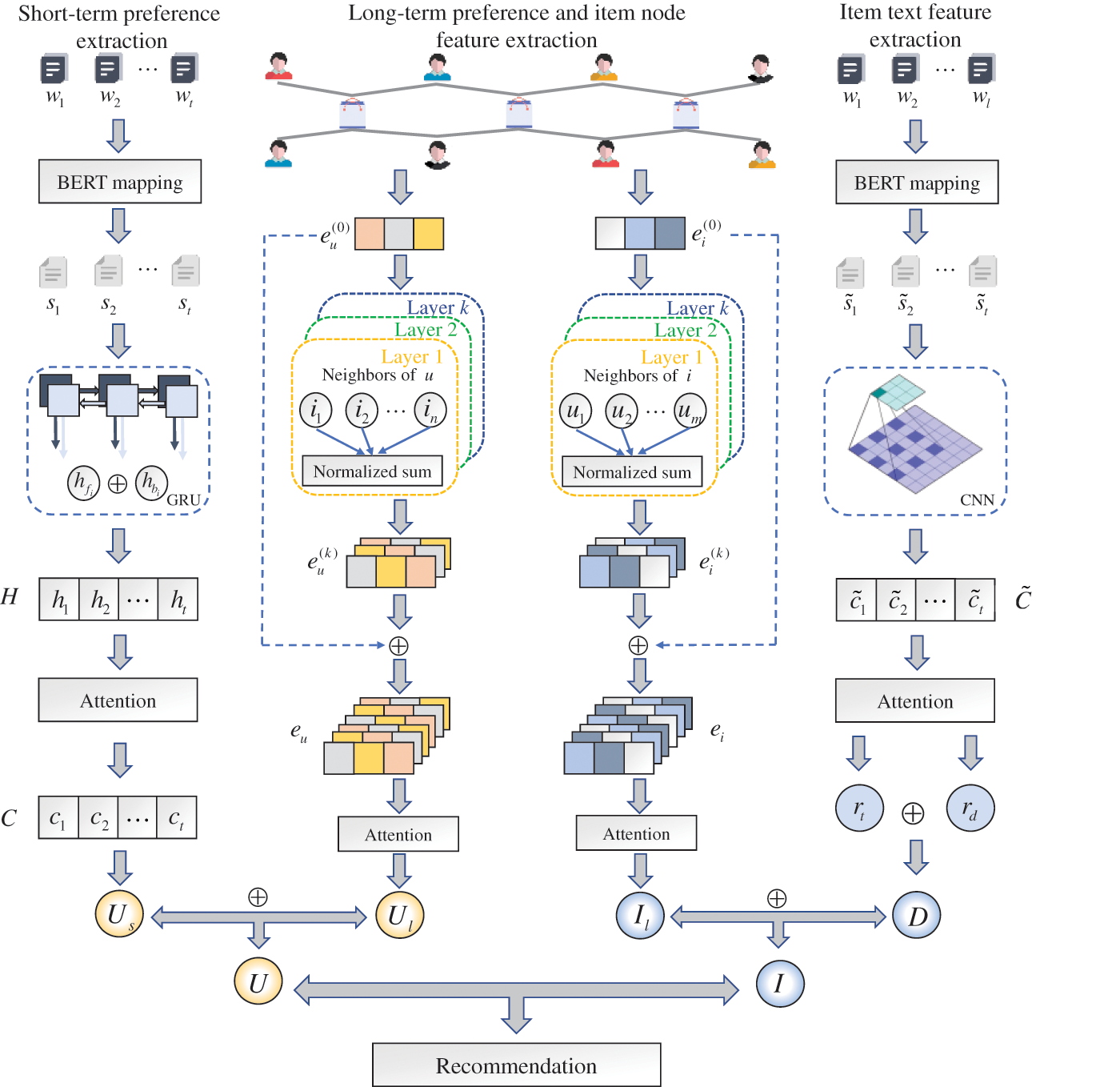
Figure 1: The overall framework of the proposed model

2.1 Long-Term Preference and Item Node Feature Extraction Module

The long-term preference and item node feature extraction module includes the long-term preference extraction of users and the node feature extraction of items. Since the extraction methods are the same, we only describe the users’ long-term preference extraction method.

2.1.1 ID Feature Embedding Layer

This layer illustrates the feature embedding representation of users and items. We construct user-item interaction graphs using the complete historical interaction data, embedding each user and item into a dense vector by their respective IDs.

If there are m users and n items, we denote the initial embedding vector of users as the set eu(0)=[eu1(0), eu2(0), …, eum(0)] and the initial embedding vector of items as the set ei(0)=[ei1(0), ei2(0), …, ein(0)] . The ID embedding vectors of users and items are in their initial state. We further refine the embedding by propagating them in the forward propagation layer so that the ID embedding vectors can better express their connoted association relationships.

2.1.2 Forward Propagation Layer

This layer computes the node representations of all users and items. We aggregate the neighboring nodes in the interaction graph by a Graph Convolutional Network (GCN) [10] and perform forward propagation to obtain the embedding representations of long-term preference and item nodes.

First, we aggregate the initial ID embeddings of the item nodes in all neighboring nodes of user u . Thus, we obtain the first layer embedding expression of user u in the GCN, as shown in Eq. (1).

eu(1)=∑i∈Nu1|Nu||Ni|ei(0) (1)

where, eu(1) denotes the first-order feature of user u on the first GCN layer, ei(0) denotes the first-order feature of item i on the first GCN layer, 1/(NuNi) denotes the aggregation operation in the original GCN design, Nu denotes the set of neighboring nodes of user u, and Ni denotes the set of neighboring nodes of item i. In short, Eq. (3) aggregates the initial item node ID embedding of all neighboring nodes of user u to obtain the first level embedding representation of user u in the interaction graph.

Then, according to the computation of first-order propagation, we can stack multilayer graph convolution in a GCN to model the higher-order association relationship features between users and items, as shown in Eq. (2).

eu(k)=∑i∈Nu1|Nu||Ni|ei(k−1) (2)

where, eu(k) denotes the features of user u on the kth GCN layer and eu(k−1) denotes the features of user u on the k−1th GCN layer.

Finally, we stitch the user node representation by layer forward propagation to obtain the final representation eu=eu(0)⊕eu(1)⊕⋯⊕eu(k) of the user node.

2.1.3 Attention Layer

This layer assigns attention weights to the different layer embeddings to determine the importance of each layer embedding.

We calculate the attention distribution α for each embedding layer, as shown in Eq. (3).

αu=Softmax(ωq×tanh⁡(ωk×euT)) (3)

where, αu contains the weights of the embedding representations from layer 0 to layer k, ωq is the weight matrix of query in the attention mechanism, ωk is the weight matrix of key in the attention mechanism, and Softmax() function is used to normalize the weights of the kth layer embedding.

We use the attention distribution to weigh and sum the embedding vectors of each layer to obtain the long-term preference representation Ul of users in the total interaction data, as shown in Eq. (4).

Ul=∑Z=0kαu(z)eu(z) (4)

Similarly, we use the methods in Sections 2.1.2 and 2.1.3 to obtain the node feature representation Il of the items in the total interaction data.

2.2 Short-Term Preference Feature Extraction Module

The short-term preference feature extraction module extracts the short-term preferences of users through their recent interaction history.

2.2.1 Item Sequence Embedding Layer

This layer transforms the sequence of the items into a low-dimensional vector output. We use Bidirectional Encoder Representation from Transformers (BERT) because BERT is composed of multiple transformer overlays, which can solve the problem of multiple meanings of a word; also, BERT can selectively utilize information from all layers, allowing the multilayer properties of words to be exploited [11].

First, given a sequence of t items with which user u has recently interacted, we obtain a textual representation W=[w1, w2, …,wt] of the corresponding items in the item sequence.

Then, to get the vector of the sequence low-dimensional, we input the item text into the BERT model, get the low-dimensional vector through the encoder, and denote the obtained vector as S=[s1, s2, …,st] .

Finally, since each item sequence has different lengths, the obtained vectors have different sizes, and too much difference in the vectors will affect the overall effect of the model. Therefore, we adopt the fixed-length strategy and select only a fixed number of low-dimensional vectors. Among them, the vectors that exceed the fixed length are truncated, and zero vectors complement the vectors that do not reach the fixed length.

2.2.2 Vector Encoding Layer

This layer captures the order information in the low-dimensional vectors. When the encoding layer encodes the word vectors, it needs to include contextual information. The standard encoders only keep the data content of the current moment and ignore the data content of the last moments, which can significantly increase the prediction error. To overcome this problem, we use Bi-directional Gated Recurrent Unit (Bi-GRU) [12] to encode the word vectors.

First, we use Bi-GRU to forward and backward encoding of the low-dimensional vectors of item information, as shown in Eqs. (5) and (6). The forward encoding performs feature extraction in the order from vector s1 to vector st . The backward encoding performs feature extraction in the order from vector st to vector st .

hfi=GRUforward(si), i∈[1, 2, …, t] (5)

hbi=GRUbackward(si), i∈[1, 2, …, t] (6)

Then, we cascade the forward features hf and backward features hb to obtain the order information features h of each item vector as a whole, as shown in Eq. (7).

hi=hfi⊕hbi, i∈[1, 2, …, t] (7)

Finally, we integrate and output the order information of each item vector as a whole, denoted as H=[h1, h2, …,ht] .

2.2.3 Attention Layer

This layer assigns different attention weights to each item vector [13], which determines the importance of the user’s recently interacted items and empowers the model to extract short-term preference features.

We calculate the attention distribution β for the importance of each interaction item, as shown in Eq. (8).

β=Softmax(ωq~×tanh⁡(ωk~×HT)) (8)

where, to distinguish from the attention mechanism of the long-term preference extraction module, we denote the weight matrix of query as ωq~ , the weight matrix of key as ωk~ , β contains the embedding representation weights of the 1st to the tth item vector, and Softmax() function is used to normalize the weights of the kth layer embedding.

We add the weight of the order information provided by the vector coding layer based on attention distribution and represent the overall feature of items’ order information as C=[c1, c2, …, ct] , which is calculated as shown in Eq. (9).

C=βH (9)

2.2.4 Feature Mapping Layer

This layer multiplies the sequential features after adding attention weights with the learnable weight matrix to get the short-term preference representation of the user, as shown in Eq. (10).

Us=ω1×C+b1 (10)

where, ω1 is the weight parameter of the feature mapping layer and b1 is the bias parameter of the feature mapping layer.

2.3 Item Text Feature Extraction Module

The item text feature extraction module extracts the textual representation of the item from the item title and description information. Due to the sparsity of the data in the RS, capturing the features of the items using IDs alone may not be sufficient, so we use this module to extract additional textual representations of the items.

2.3.1 Item Sequence Embedding Layer

This layer embeds the title and description information of the items. We obtain the vector sequence S~=[s~1, s~2, …,s~t] of item title and description information by the method shown in Section 2.1.1.

2.3.2 Convolutional Neural Network Layer

This layer captures the hidden contextual word representations in the item words. The local context of words in the input text is essential for learning their representations. Therefore, we design a Convolutional Neural Network (CNN) to learn contextual word learning by capturing its local context.

We denote the contextual word sequence of items as C~=[c~1, c~2, …,c~t] , and its convolution is calculated as shown in Eq. (11).

c~i=Relu(ω2×S~i±k+b2) (11)

where, s~i±k is the vector sequence stitching from position i−k to i+k , ω2 is the convolutional kernel weight of the CNN filter, b2 is the bias parameter of the CNN filter, and Relu() is the activation function.

After the convolutional computation, we design the attention mechanism to assign different attention weights to contextual words to select the essential words in the context.

We calculate the attention weight χ for each word in the sequence, as shown in Eq. (12).

χ=exp⁡(tanh⁡(ω3×C~)+b3) (12)

where, ω3 is the weight parameter of word attention and b3 is the bias parameter of word attention.

We assign impact to each input text according to the attention weights and obtain the feature representation r of the word context, as shown in Eq. (13).

r=χC~ (13)

We input the title and description information of the item into this module to obtain the title representation rt of the item and the description representation rd of the item. Then, we cascade the two representations to obtain the textual feature representation D of the item as a whole, as shown in Eq. (14).

D=rt⊕rd (14)

2.4 Prediction Module

The prediction module cascades long- and short-term preference features and item text features for the final prediction of the matching score.

We cascade the long-term preference representation of the user with the short-term preference representation to obtain the final representation of the user, as shown in Eq. (15).

U=Ul⊕Us (15)

Similarly, we cascade the item’s long-term preference representation with the item’s text feature representation to obtain the final representation of the item, as shown in Eq. (16).

I=Il⊕D (16)

Finally, we inner-product the user’s final representation with the item’s final representation to predict the matching score of their interaction, as shown in Eq. (17).

r⌢ui=UT⊗I (17)

2.5 Model Objective Function

We train and optimize the model using the BPR loss function to predict the interactions between users and items. In the BPR loss function, observed interactions are assumed to represent the user’s preferences better, so higher prediction values are produced than unobserved interactions [14]. This objective function is defined as shown in Eq. (18).

Loss=∑(u,i,j)∈o−ln⁡σ(r^ui−r^uj)+λ‖θ‖22 (18)

where, o={(u, i, j)|(u, i)∈R+, (u, j)∈R−} is the pairwise training data, R+ is the observed interaction, R− is the unobserved interaction, σ() is the activation function, we choose the sigmoid function, θ={ωq, ωk, ωq~, ωk~, ω1, b1, ω2, b2, ω3, b3} is the set of all trainable parameters of the model and λ controls the L2 regularization strength to prevent overfitting.

3  Experiment and Analysis

In this section, we perform experiments on the Amazon public dataset, which consists of parameter optimization experiments, performance analysis experiments, ablation experiments, and case analysis to confirm the effectiveness of LSGNN from various aspects.

3.1 Datasets

The Amazon dataset, one of RS’s most widely used datasets [15], has a large dataset to support our experiments. Therefore, we choose five datasets with review text in the Amazon dataset as the datasets for our experiments, namely Automotive (Auto), Baby, Sports & Outdoors (SO), Video_Games (VG), and Toys_and_Games (TG). The number of users, number of items, number of interactions, and data sparsity are shown in Table 1. To ensure feasibility and fairness, we randomly divide each dataset into a training set, a test set, and a validation set in the ratio of 7:2:1. On the validation set, we debug the optimal parameters. On the test set, we evaluate the model’s performance.

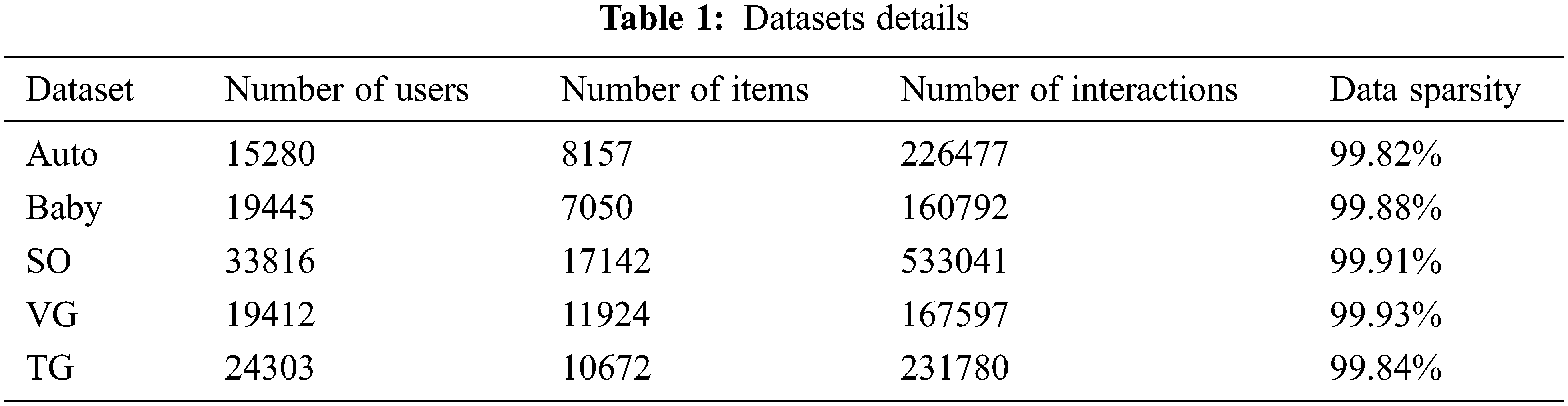
As seen in Table 1, although the data for each sample differed considerably, these datasets are sufficient to train and validate the proposed model because the data is large enough. In addition, the sparsity of each dataset is above 99%, which illustrates the significance of our adding item text features to alleviate sparsity.

3.2 Experimental Setup

3.2.1 Evaluation Metrics

Since the recommendation rating prediction is essentially a regression problem, we use the Root Mean Square Error (RMSE) and the Mean Square Error (MSE) [16], the most common evaluation metrics for regression problems, as shown in Eqs. (19) and (20), respectively.

RMSE=1|Z|∑u∈Z,i∈Z(r^ui−rui)2 (19)

MSE=1|Z|∑u∈Z,i∈Z(r^ui−rui) (20)

where, Z is the number of interactions, r^ui is the predicted rating of item i by user u, and rui is the actual rating of item i by user u. The smaller the RMSE and MSE, the lower the model’s prediction error and the higher the prediction accuracy.

3.2.2 Baselines

We classify the baselines into three categories: traditional recommendation method (BPRMF), long- and short-term preference-based recommendation methods (CLSR, LSMA, and SLSTNN), and GNN-based recommendation methods (LightGCN, HA-GNN, and LDGC-SR).

BPRMF [17]: The Bayesian Personalized Ranking (BPR) matrix factorization method allows the interaction information to be used directly as the final target value.

CLSR [18]: The short-term interest representation of users is learned using the self-attention mechanism, the long-term features of users are extracted using Bi-GRU, and finally, the long- and short-term features are fused.

LSMA [19]: Combines multilayer attention mechanisms and spatiotemporal information to model users’ long- and short-term preferences and studies users’ preferences at a coarse-grained semantic level.

SLSTNN [20]: Improves the representation of spatiotemporal data by combining a two-layer attention mechanism and a long and short-term neural network.

LightGCN [21]: Uses a GCN to model user-items higher-order connectivity and simplifies the GCN’s redundant parts.

HA-GNNN [22]: Dependencies between items are captured using a self-attentive GNN, the higher-order relationships in the graph are learned using a soft-attention mechanism, and finally, the embeddings of items are updated using a fully connected layer.

LDGC-SR [23]: Global contextual information of nodes is integrated using normalization and adaptive weight fusion mechanisms, and the current interest of users is captured more accurately by a global context-enhanced short-term memory module.

3.2.3 Parameter Setting

To better improve the recommendation effect of the model, we debug the essential parameters of the model.

We choose the appropriate GNN embedding dimension in {16, 32, 64}, and the results are shown in Fig. 2. The best result is achieved when the embedding dimension of the GNN is 32. However, the model performance is worse when the embedding dimension is larger, which may be because the overfitting of the model is caused by too large embedding dimension. Therefore, we set the GNN embedding dimension to 32.

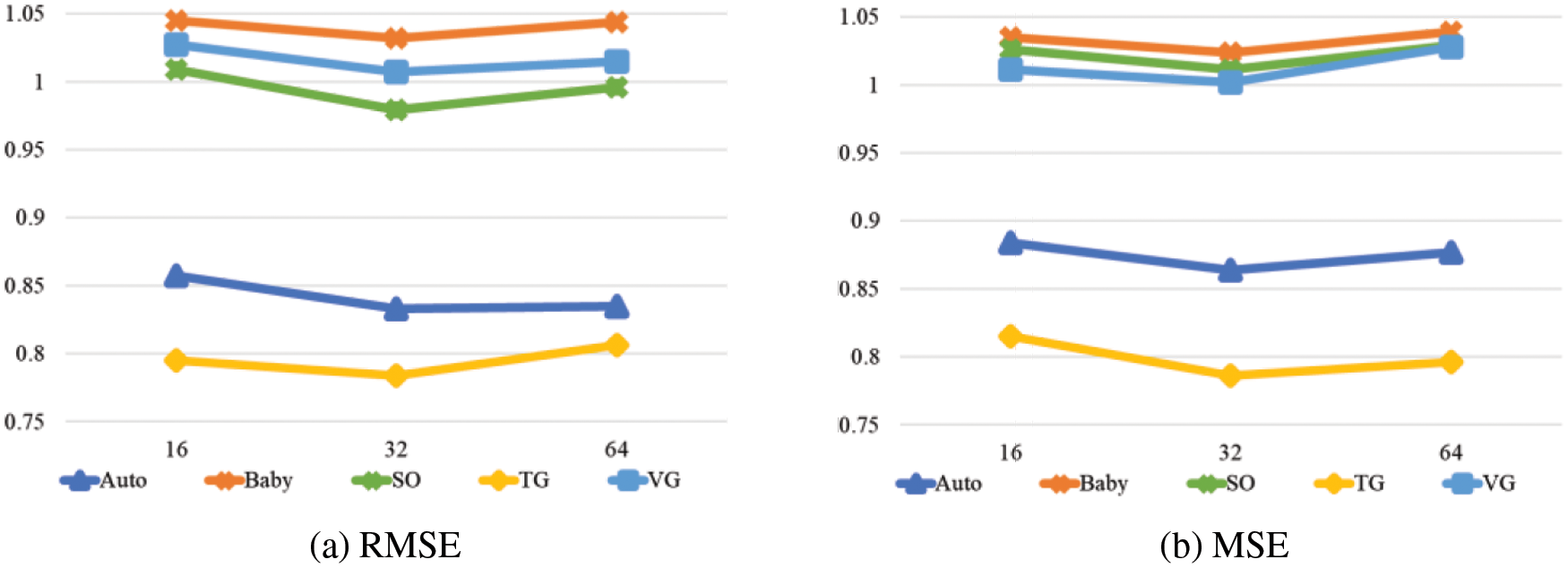
Figure 2: The effect of GNN embedding dimension on the model

We choose the appropriate GNN layers in {1, 2, 3, 4}, and the results are shown in Fig. 3. The number of GNN layers achieves the best result at layer 3. At the same time, deeper GNN layers do not improve the model’s performance much, which may be because of the model smoothing, as the representation between nodes is too similar after multilayer neighborhood aggregation. Therefore, we set the GNN layers to 3.

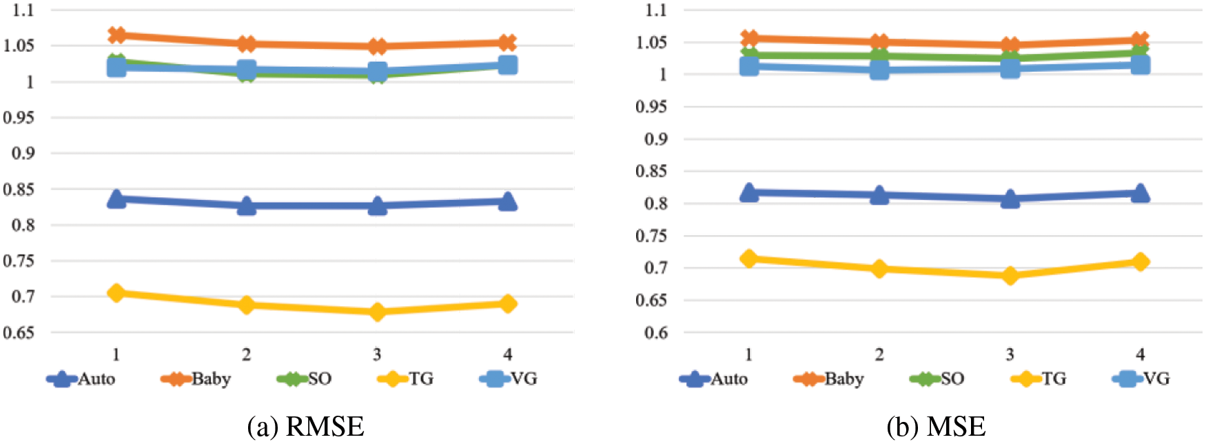
Figure 3: The effect of GNN layers on the model

We choose the appropriate word embedding dimension for item text in {50, 100, 200, 300}, and the results are shown in Fig. 4. There is no significant improvement in model performance as the word embedding dimension increases, which may be because the smaller word embedding dimension captures enough implicit information. Therefore, to speed up the model’s training, we set the word embedding dimension to 50.

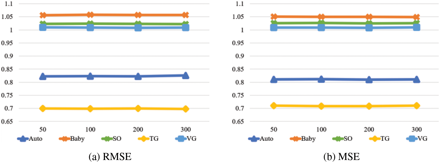
Figure 4: The effect of word embedding dimension on the model

We choose the appropriate number of recent interaction items in {1, 3, 5, 7, 9, 11} and use these items as the sequence of items used in the user’s short-term preference extraction. The results are shown in Fig. 5. As the number of recent interactions increases, the best model performance is achieved when the number is 7, which proves that combining user short-term preference features can improve the recommendations’ performance. However, when the number of recent interactions is higher, the model’s performance starts to decrease, which may be because too many interactions make the short-term preference representation similar to the long-term preference representation, and combining similar feature representations reduces the model’s expressiveness. Therefore, we set the number of recent interaction items to 7.

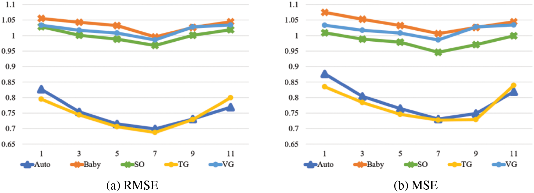
Figure 5: The effect of the number of recent interaction items on the model

3.3 Experimental Results and Comparison

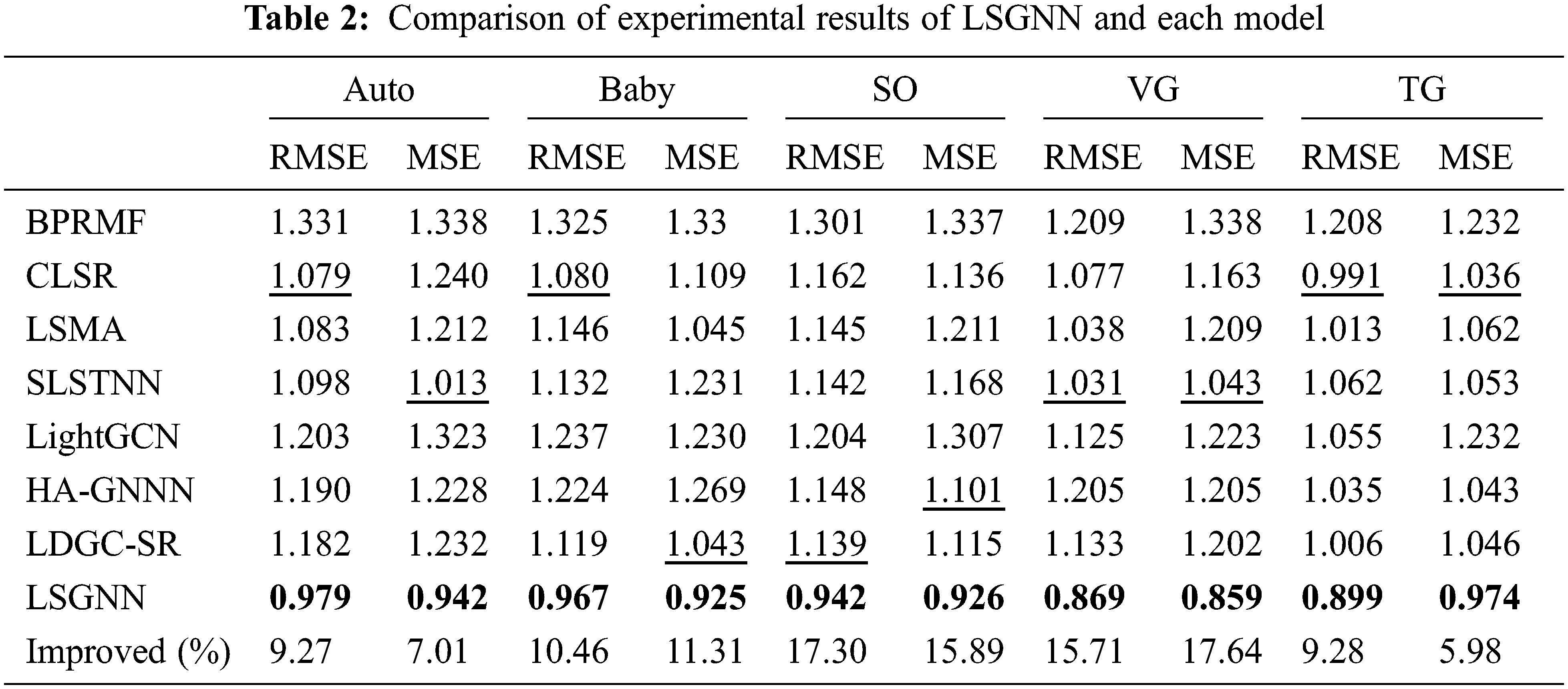
We conducted experiments with optimal parameters, set the optimal parameters for each model by corresponding literature, and compared each model’s RMSE and MSE metrics under the optimal parameters. The results are shown in Table 2. Among them, the bolded data are the best results in the same group of comparison experiments, the underlined data are the second-best results in the same group of comparison experiments, and the Improved value is the growth ratio of the best effect compared with the second-best effect. As seen from Table 2, the LSGNN model proposed in this paper has the best overall performance, as expected.

To visually analyze the effectiveness of the fusion of long- and short-term preferences and the effectiveness of the proposed model, we show histograms for each model on five datasets, as shown in Fig. 6.

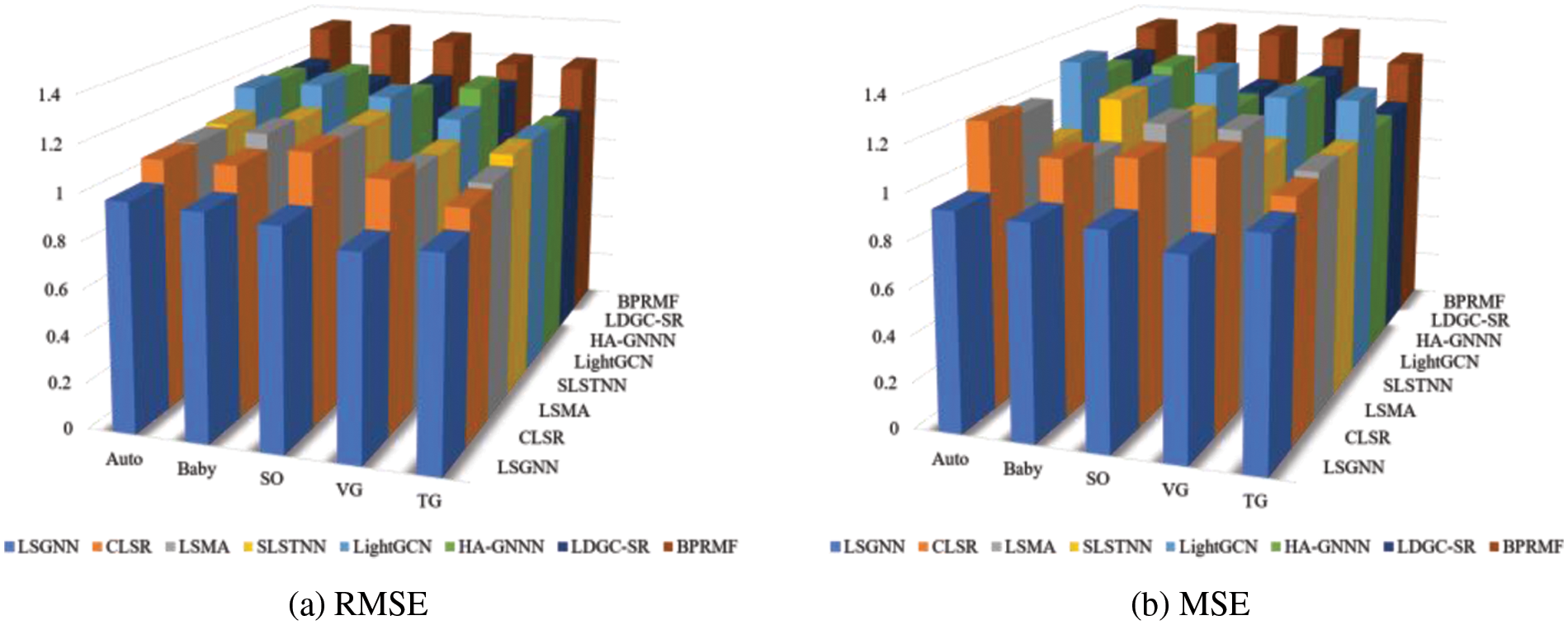
Figure 6: The effect comparison histogram

First, the traditional recommendation method (BPRMF) has the worst results for both metrics, which indicates that a simple interaction multiplication of user-item interaction information cannot capture the hidden higher-order relationships between users and items. Thus, its recommendation performance does not perform well in datasets with large amounts of data.

Second, the GNN-based recommendation methods (LightGCN, HA-GNN, and LDGC-SR) achieve better results than the traditional recommendation method, which demonstrates the superior performance of GNN in capturing higher-order relationships. Specifically, LightGCN simplifies the embedding process by removing nonlinear activation and feature transformations but does not consider the importance of each node embedding. HA-GNN utilizes an attention mechanism to learn hidden features and a fully connected layer to learn the representation of multimodal features, which has achieved good results in extracting node features using GNN. LDGC-SR uses a normalization and adaptive weight fusion mechanism with a global context-enhanced short-term memory module to capture more latent information from recent interactions and neighboring sessions, thus achieving the best experimental results among the GNN-based methods.

Third, the long- and short-term preference-based recommendation methods (CLSR, LSMA, and SLSTNN) achieve in most cases due to the traditional recommendation method and GNN-based recommendation methods. Specifically, CLSR models users’ recent behaviors, uses a self-attentive mechanism for long-term preference mining and combines long- and short-term to solve the sequential recommendation problem. Although CLSR works well for the extraction of user-item interactions, it does not consider data other than the interactions and thus needs to be improved. LSMA constructs long-term preference modeling through LSTM, achieves short-term preference modeling through RNN and attention mechanism, and can mine users’ motion behavior models through a multilayer attention mechanism. Although LSMA models long- and short-term preferences through temporal sequences well, it only models interaction data without considering other attributes, so it needs to be improved. SLSTNN represents user long- and short-term sequences through a hierarchical attention mechanism and uses a feature crossover network to achieve feature representation to recommend more beneficial orders for online taxi drivers. Although the recommendation effect of SLSTNN makes the order completion rate much higher, it is too single in its modeling objectives and does not integrate more objectives into the model, so it needs improvement.

Finally, our proposed LSGNN works better than the other baselines in every dataset. In particular, in two datasets with high sparsity, SO and VG, the improvement of LSGNN is higher than several in other datasets, which proves that LSGNN plays a role in alleviating data sparsity. Meanwhile, by fusing long and short-term preference features and item text features, LSGNN can extract deeper hidden features in interaction information and obtain more acceptable user preferences, thus achieving better recommendation results.

3.4 Analysis of Ablation Experiments

To further verify the effectiveness of the LSGNN model, we do ablation experiments for the critical parts of the model, long-term preference and item node feature extraction module, short-term preference feature extraction module, and item text feature extraction module, and select the experimental results on SO and VG datasets with high sparsity to demonstrate the results as shown in Table 3, where LSGNN-LP is the model with only long-term preference and item node feature extraction module, LSGNN-SP is the model with only short-term preference extraction module, and LSGNN-IT is the model with item text feature extraction module removed.

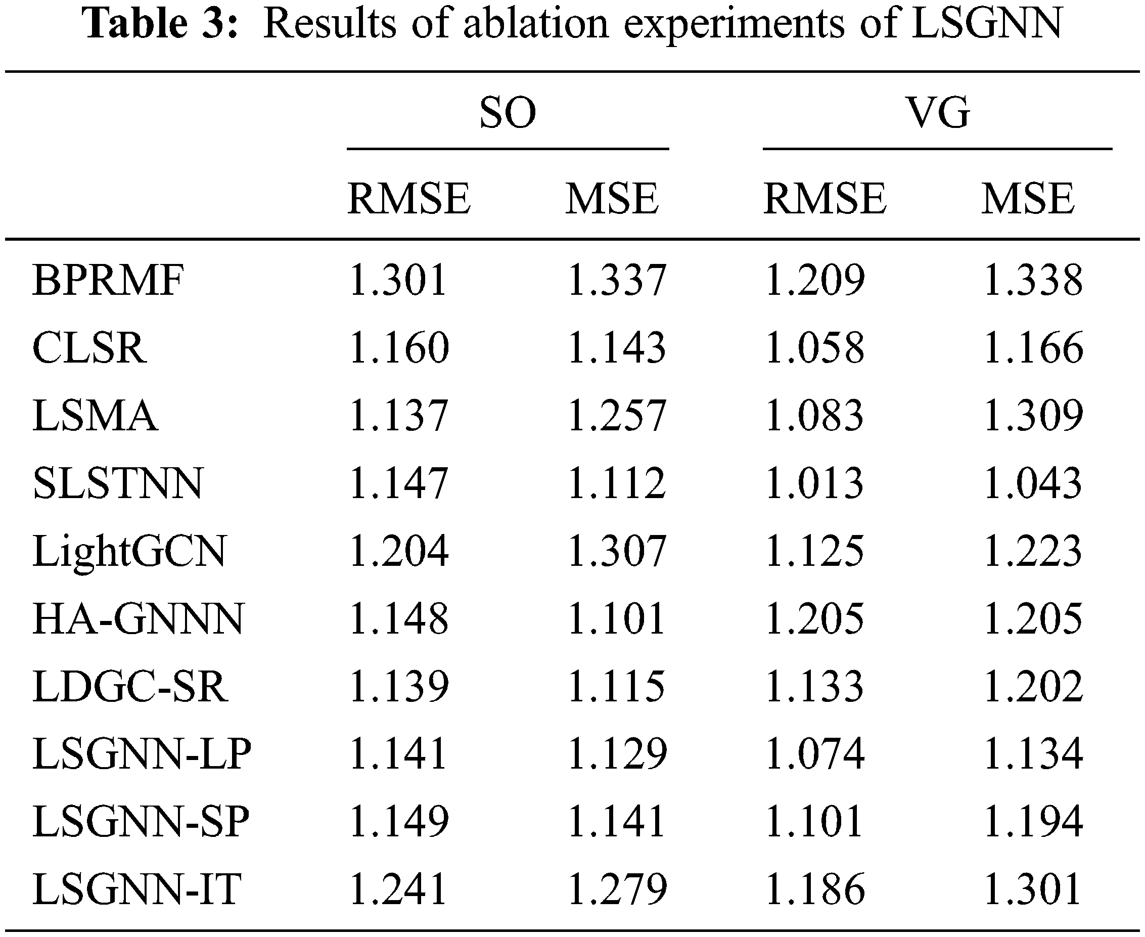
First, the model with only a long-term preference and item node feature extraction module outperforms the absolute majority of models in the baselines, which is because LSGNN-LP uses an attention mechanism on top of GNN to obtain feature representations on all interaction graphs, which further optimizes the performance of GNN in learning long-term preferences by targeting node embeddings based on the attention weights.

Then, the model with only a short-term preference feature extraction module achieves good recommendation results because LSGNN-SP introduces the BERT as an embedding layer that can effectively extract semantic information from interaction data. Meanwhile, the Bi-GRU combined with the attention mechanism can capture the contextual information of words from both directions, enabling the model to more accurately capture the meanings expressed in the recent interaction data and focus on more relevant recent preferences.

Finally, the effect of the model after removing the item text feature extraction module is lower than most of the models in the baselines, because when no data or attributes other than the interaction graph are added, it will cause data sparsity on the one hand. On the other hand, it will lead to over-fusion of data leading to repeated interactions, which reduces the recommendation effect after fusion.

In summary, the roles and effects in each module of LSGNN achieve good results.

3.5 Case Analysis

To better understand the recommendation process, we take the user with ID 232 in dataset Auto as an example and use 3-hop propagation with Top10 recommendations for the case study. The specific process is shown in Fig. 7. First, user 232 constitutes the first embedding, i.e., embedding_0 . Second, the first-order neighbors of user 232, i.e., their direct purchases, are items 16, 375, 7296, etc., which generate the first-order embedding of user 232, i.e., embedding_1 . We take the next hop of item 16 as an example. Item 16 has been purchased by users 40, 211, 4696, i.e., it is part of the second-order neighbors of user 232. All second-order neighbors are aggregated to get the second-order embedding of user 232, i.e., embedding_2 . Similarly, all third-order neighbors are aggregated to get the third-order embedding of user 232, i.e., embedding_3 .

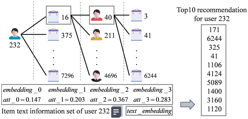
Figure 7: Case analysis

The attention mechanism assigns attention weights of 0.147, 0.203, 0.367, and 0.283 to each order of embedding. From the weights, we can see that the second-order embedding has the largest weight, followed by the third-order embedding. This indicates that the second-order embedding plays an essential role in the end-user representation and verifies the validity of choosing 3 layers for the GNN layers. After adding the attention weights, long- and short-term preferences for interactions are generated.

The item text information set of user 232 is generated by the BERT and a CNN to generate the item text feature embedding text_embedding . This feature embedding is co-guided with the interactive long- and short-term preference embedding to give the item recommendation sequences of user 232, i.e., item 171, 6244, 325, etc. The presence of item 6244 and item 41 in the item recommendation sequence is observed. The recommendations of these two items are consistent with the embedding generation process in the previous graphs, demonstrating the interpretability of our proposed model LSGNN.

4  Conclusion

In this paper, we propose a GNN recommendation model based on long- and short-term preference, called LSGNN. This model extracts long-term preferences by a GNN combined with the attention mechanism, short-term preferences by the Bi-GRU combined with the attention mechanism and item text features by a CNN combined with the attention mechanism, and fuses these features to achieve recommendations. LSGNN showed better performance than the baselines on five publicly available datasets from Amazon.

In future research work, we will extend our work in two directions: first, the complexity of the model leads to the low speed of recommendations, especially for machines with insufficient arithmetic power, so we intend to simplify the structure of the model to speed up the recommendations without affecting the results. Second, since the interaction data is too large to be simply randomly sampled, we intend to design a sampling strategy that improves the performance of the recommendation while speeding it up.

Acknowledgement: We would like to sincerely thank all those who have provided support and assistance in this research. We are grateful to our advisors and laboratory colleagues for their guidance and collaboration, which have made this study possible. We also want to express our gratitude to our families and friends for their continuous encouragement and support.

Funding Statement: This research was supported by the National Natural Science Foundation of China under Grant 61762031, the Science and Technology Major Project of Guangxi Province under Grant AA19046004, the Natural Science Foundation of Guangxi under Grant 2021JJA170130, the Innovation Project of Guangxi Graduate Education under Grant YCSW2022326, and the Research Project of Guangxi Philosophy and Social Science Planning under Grant 21FGL040.

Author Contributions: The authors confirm contribution to the paper as follows: study conception and design: Bohuai Xiao, Xiaolan Xie; data collection: Chengyong Yang; analysis and interpretation of result: Bohuai Xiao; draft manuscript preparation: Bohuai Xiao, Xiaolan Xie. All authors reviewed the results and approved the final version of the manuscript.

Availability of Data and Materials: Due to the nature of this research, participants of this study did not agree for their data to be shared publicly, so supporting data is not available.

Conflicts of Interest: The authors declare that they have no conflicts of interest to report regarding the present study.

References

1. J. Bobadilla, F. Ortega, A. Hernando and A. Gutierrez, “Recommender systems survey,” Knowledge-Based Systems, vol. 46, pp. 109–132, 2013. [Google Scholar]

2. M. An, F. Wu, C. Wu, K. Zhang, Z. Liu et al., “Neural news recommendation with long-and short-term user representations,” in 57th Annual Meeting of the Association for Computational Linguistics, Florence, Italy, pp. 336–345, 2019. [Google Scholar]

3. Q. Chen, H. Zhao, W. Li, P. Huang and W. Ou, “Behavior sequence transformer for e-commerce recommendation in alibaba,” in 1st Int. Workshop on Deep Learning Practice for High-Dimensional Sparse Data, New York, NY, USA, pp. 1–4, 2019. [Google Scholar]

4. R. Berg, T. N. Kipf and M. Welling, “Graph convolutional matrix completion,” arXiv preprint arXiv:1706.02263, 2017. [Google Scholar]

5. R. Ying, R. He, K. Chen, E. Pong and H. William, “Graph convolutional neural networks for web-scale recommender systems,” in 24th ACM SIGKDD Int. Conf. on Knowledge Discovery & Data Mining, London, UK, pp. 974–983, 2018. [Google Scholar]

6. J. Zhang, X. Shi, S. Zhao and I. King, “Star-gcn: Stacked and reconstructed graph convolutional networks for recommender systems,” arXiv preprint arXiv:1905.13129, 2019. [Google Scholar]

7. B. Wang, X. Lyu, J. Qu, H. Sun, Z. Pan et al., “GNDD: A graph neural network-based method for drug-disease association prediction,” in 2019 IEEE Int. Conf. on Bioinformatics and Biomedicine (BIBM), San Diego, USA, IEEE, pp. 1253–1255, 2019. [Google Scholar]

8. A. Sanchez-Gonzalez, N. Heess, J. T. Springenbergs, J. Merel, M. Riedmiller et al., “Graph networks as learnable physics engines for inference and control,” in 35th Int. Conf. on Machine Learning, Stockholm, Sweden, vol. 80, pp. 4470–4479, 2018. [Google Scholar]

9. W. Chiang, X. Liu, S. Si, Y. Li, S. Bengio et al., “Cluster-gcn: An efficient algorithm for training deep and large graph convolutional networks,” in 25th ACM SIGKDD Int. Conf. on Knowledge Discovery & Data Mining, New York, NY, USA, pp. 257–266, 2019. [Google Scholar]

10. T. N. Kipf and M. Welling, “Semi-supervised classification with graph convolutional networks,” arXiv preprint arXiv:1609.02907, 2016. [Google Scholar]

11. G. Penha and C. Hauff, “What does bert know about books, movies and music? Probing bert for conversational recommendation,” in 14th ACM Conf. on Recommender Systems, New York, NY, USA, pp. 388–397, 2020. [Google Scholar]

12. Y. Zhang, P. Zhao, Y. Guan, L. Chen, K. Bian et al., “Preference-aware mask for session-based recommendation with bidirectional transformer,” in 2020–2020 IEEE Int. Conf. on Acoustics, Speech and Signal Processing (ICASSP), Barcelona, Spain, pp. 3412–3416, 2020. [Google Scholar]

13. A. Vaswani, N. Shazeer, N. Parmar, J. Uszkoreit, L. Jones et al., “Attention is all you need,” Advances in Neural Information Processing Systems, vol. 30, pp. 6000–6010, 2017. [Google Scholar]

14. S. Guo, C. Chen, J. Wang, Y. Liu, K. Xu et al., “Rod-revenue: Seeking strategies analysis and revenue prediction in ride-on-demand service using multi-source urban data,” IEEE Transactions on Mobile Computing, vol. 19, no. 9, pp. 2202–2220, 2019. [Google Scholar]

15. T. D. Noia, V. C. Ostuni, P. Tomeo and E. D. Sciascio, “Sprank: Semantic path-based ranking for top-n recommendations using linked open data,” ACM Transactions on Intelligent Systems and Technology, vol. 8, no. 1, pp. 1–34, 2016. [Google Scholar]

16. X. Huang, Y. Ye, C. Wang and L. Xiong, “A multi-mode traffic flow prediction method with clustering based attention convolution LSTM,” Applied Intelligence, pp. 1579–7497, 2021. [Online]. Available: https://link.springer.com/article/10.1007/s10489-021-02770-z [Google Scholar]

17. S. Rendle, C. Freudenthaler, Z. Gantner and L. Schmidt-Thieme, “BPR: Bayesian personalized ranking from implicit feedback,” arXiv preprint arXiv:1205.2618, 2012. [Google Scholar]

18. L. Niu, Y. Peng and Y. Liu, “Deep recommendation model combining long-and short-term interest preferences,” IEEE Access, vol. 9, pp. 166455–166464, 2021. [Google Scholar]

19. X. Wang, Y. Liu, X. Zhou, Z. Leng and X. Wang, “Long-and short-term preference modeling based on multi-level attention for next POI recommendation,” ISPRS International Journal of Geo-Information, vol. 11, pp. 323–340, 2022. [Google Scholar]

20. X. Sheng, F. Wang, Y. Zhu, T. Liu and H. Chen, “Personalized recommendation of location-based services using spatio-temporal-aware long and short term neural network,” IEEE Access, vol. 10, pp. 39864–39874, 2022. [Google Scholar]

21. X. He, K. Deng, X. Wang, Y. Li, Y. Zhang et al., “LightGCN: Simplifying and powering graph convolution network for recommendation,” in 43rd Int. ACM SIGIR Conf. on Research and Development in Information Retrieval, New York, NY, USA, pp. 639–648, 2020. [Google Scholar]

22. S. Sang, N. Liu, W. Li, Z. Zhang, Q. Qin et al., “High-order attentive graph neural network for session-based recommendation,” Applied Intelligence, pp. 1573–7497, 2022. [Online]. Available: https://link.springer.com/article/10.1007/s10489-022-03170-7 [Google Scholar]

23. N. Qiu, B. Gao, H. Tu, F. Huang, Q. Guan et al., “LDGC-SR: Integrating long-range dependencies and global context information for session-based recommendation,” Knowledge-Based Systems, vol. 248, pp. 108894, 2022. [Google Scholar]