Micro-Locational Fine Dust Prediction Utilizing Machine Learning and Deep Learning Models

1  Introduction

Owing to rapid urbanization, both social and economic issues related to environmental pollution have been consistently highlighted. Among the several aspects of environmental pollution, air pollution is one of the notable threats to human health. The infamous ‘the London smog event’, which occurred in December 1952 in London, England, reportedly resulted in the tragic loss of approximately 12,000 residents’ lives [1]. Recently, air pollution has become a major problem, threatening human health and causing deaths [2]. Air pollution is typically described as the presence of detrimental substances in the air at levels that can endanger one’s health [3]. It is primarily caused by well-known noxious substances known as air pollutants. Air pollutants are substances that can harm humans, animals, vegetation, or materials, with particulate matter (PM) and gaseous species (NO2, CO, O2, and SO2) being major components [4]. These pollutants have detrimental effects on human health and the economy [5], leading to significant environmental and societal problems [6]. Specifically, PM2.5 and PM10 particles, which have diameters less than 2.5 and 10 micrometers, respectively, have diverse adverse effects on human health. They are a major contributor to health crises [7], and human exposure to PM can result in various critical and chronic diseases, including cardiovascular and respiratory issues such as asthma [8,9].

The adverse impacts of fine dust have been widely addressed. Prior research has demonstrated the notable negative effects of fine dust on the national economy [10,11]. Fine dust can significantly affect the entire production and delivery processes of high-tech industries that require an environment related and dust-free workspace (e.g., semiconductor industry [10]). Moreover, because fine dust causes avoidance of outdoor activities, the local economy and industries significantly related to outdoor activities (e.g., tourism industry) are negatively affected [10,12]. With regard to the macro aspects of fine dust effects, prior research has reported that fine dust concentrations might have caused approximately 700 deaths in January 2013, Beijing, China, while health-related economic loss is estimated at 253.8 million USD [13]. In addition, reference [11] argued that the total socioeconomic cost of yellow dust, which is one of the comprehensive terms used for fine dust, was estimated annually to range between 3,900 and 7,300 million USD [14].

Therefore, it is crucial to effectively inform and manage the levels of fine dust to prevent negative social and economic outcomes. Predicting air quality impacted by fine dust has been a focus in guiding citizens’ activities and reducing industrial and economic costs [10]. To achieve this, accurate prediction of fine dust levels for all locations is essential to provide necessary information to the entire population of a country. However, this need is often unmet due to the lack of observatories. One of the main challenges is the imbalance in the distribution of fine dust observatories, resulting in a significant number of areas lacking accurate observations on fine dust. For example, in Nowy Targ, a tourist town in Poland, the nearest air quality monitoring station is approximately 30 km away due to the absence of observation stations in residential and mountainous areas [15]. Considering several difficulties in establishing air pollution monitoring stations in urban areas, it is required to explore data-centric approaches for predicting fine dust levels at micro-locations.

In the case of South Korea, micro-observations on fine dust are one of the most challenging academic and practical problems as well because of the characteristics of residential environments and topographic issues. The shortage of observation stations in cities and provinces, except for metropolitan areas, has also been highlighted in South Korea. This is because stations are typically installed based on the principle of population density restriction [16], which means a limited number of accurate and minute air quality observations in small towns and areas. For instance, the average coverage of observation stations in a rural area is seven times lower than that of the South Korean capital city (Seoul [17]).

According to the Ministry of Environment in South Korea [16], several prerequisites are required to establish observation stations. For instance, urban atmosphere observation stations should be located in cities with populations greater than 100 thousand. Moreover, the observation stations should have no external regional influences. In addition to the above conditions, geographical factors are also important for establishing atmospheric observation stations, indicating that installing additional observation stations is difficult. Therefore, a few studies have examined the problems in the existing systems and proposed alternative observation equipment.

Reference [18] highlighted the limitations of the National Ambient Air Monitoring Information System (NAMIS) in South Korea. It highlighted the shortage of air observation stations as a significant factor contributing to the low reliability of fine dust observations. In situations where a specific location lacks an observatory, the air quality at that point is estimated by averaging the observation values from nearby observatories. Consequently, for users located outside the service area, the provided information can be inaccurate depending on their real-time location. Furthermore, it suggested the need to introduce a greater number of cost-effective atmospheric environment monitoring systems due to various limitations in the current NAMIS in South Korea [19]. To provide a better and effective understanding of air quality topics including fine dust predictions, data-driven approaches to air quality have recently been highlighted.

Several scholars have used meteorological features and spatiotemporal information, as well as air pollutants, to examine fine dust predictions. Reference [20] examined a correlation analysis between meteorological factors and PM2.5 using a back propagation neural network (BPNN). In addition, the authors applied an autoregressive integrated moving average (ARIMA) model for short-term prediction of PM2.5 in Beijing, China by collecting a series of meteorological, air pollutant, and social media datasets from several regions. A notable correlation between the average wind speed and PM2.5 (Rn = − 0.436, p < 0.001) was indicated by the results of the correlation analysis. The following five variables were specifically considered; meteorological factors, pollutant concentrations, daily number of particular miniblog posts, all meteorological and pollutant and microblog elements, and employed elements (e.g., average wind speed, concentration of carbon monoxide (CO), nitrogen dioxide (NO2)). With this approach, they achieved root mean squared error (RMSE) scores of 24.06 (BPNN) and 6.76 (ARIMA).

Reference [21] predicted the urban air quality in India employing linear and nonlinear models including partial least squares regression, multivariate polynomial regression, and artificial neural network (ANN) models. Three different ANN models were employed: multilayer perceptron, radial-basis function network, and generalized regression neural network. They also used air and meteorological datasets for a five-year period, collected by the Central Pollution Control Board and the Indian Institute of Sugar Cane Research. The results of the models demonstrated an RMSE of 13.32 in predicting SO2 and NO2.

Reference [22] suggested a long-short term memory (LSTM)-oriented approach for computing PM10 and PM2.5 in Seoul, Korea. The air quality dataset of Seoul was used and 25 stations in separate districts of Seoul were selected. Then, 25 different LSTM-based models were trained to predict the PM10 and PM2.5 levels at each station. The resulting mean squared errors (MSE) for the 25 different models were below 0.00045. Their prediction models considered locational differences, with only a small number of stations considered in their analysis. Reference [23] predicted the grades of fine dust PM10. Based on the air quality data from 2010 to 2015 in six major metropolitan areas of Korea, they performed two classification tasks: four-grade (“Good, Moderate, Bad, Very Bad”) and two-grade (“Good or Moderate” and “Bad or Very Bad”). A deep neural network (DNN) model was used and the results of the neural network (NN), support vector machine (SVM), multinomial logistic regression (MLR), and random forest (RF) were compared. The best performance in four-grade classification (77.93%) was demonstrated by the DNN model, whereas the best accuracy in two-grade classification (97.05%) was presented by SVM, RF, and DNN models. However, their analysis had notable data imbalances and low-sensitivity issues (lower than 50%). Moreover, they did not consider continuous and time-series values in the analysis.

With this viewpoint, several scholars have attempted to address potential features with notable impacts on fine dust predictions. Reference [24] analyzed washout effects of precipitation on PM10 and NO2 in Seoul, Korea. The inter-event time definition, which is the minimum dry days between two rainfall days, was utilized to analyze the relationship between precipitation and PM10. The average PM10 was reported as noticeably different under different rainfall conditions, with lower values under rainfall conditions than under non-precipitation conditions. The following log equation for the precipitation-induced reduction effect in PM10 was proposed:

y=−4.83ln(x)−3.385(1)

The effects of air monitoring sites were also analyzed. The rainfall-induced reduction in PM10 was lower at roadside sites than urban sites because of continuous pollutant emissions from traffic at the former locations. Reference [25] presented diffusion effects of wind velocity levels on PM10. A multiple regression analysis was applied on a three-year air quality data of Seoul, Korea. A strong effect of wind speed on PM10 was indicated by the result that a higher wind speed led to lower PM10 levels.

Thus, our study aims to apply data-driven approaches to predict fine dust concentration (PM10) in specific micro-locations implementing South Korean continuous location features. For time series consideration, LSTM networks along with other regression machine learning models such as XGBoost, Adaboost, and Random Forest were leveraged. Leveraging LSTM networks, the authors tried to capture complex temporal dependencies, enhancing forecasting accuracy. This work addresses gaps in the literature, particularly the utilization of micro-geographical information and diverse time-series data sources to better observe fine dust levels in areas lacking observatories.

2  Method

2.1 Data Collection and Description

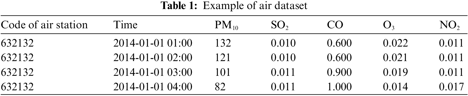
South Korean air quality and meteorological datasets were used in this study. Since 1995, the Korean government has been obligated to install an automatic air pollution measurement network to automatically measure harmful substances in the air and identify air pollution. The Ministry of Environment Korea has specified by statute the measurement and collection of the concentration levels of specific substances, such as sulfur dioxide (SO2), carbon monoxide (CO), ozone (O3), nitrogen dioxide (NO2), and fine dust (PM10, PM2.5) at one-hour intervals. The pollutant data utilized in this study were obtained from the Korean Ministry of Environment, and a variety of air datasets were made available through AirKorea [26]. Datasets spanning from January 2014 to December 2020 were collected, encompassing air-related information for each measurement station in Korea. In total, the dataset consisted of approximately 23 million samples, with an average of 11 features from 957 stations. It is worth noting that the collected datasets were limited to a period where there were no missing or unobserved hourly measurements of PM10, which was the target variable in this study. An example of a collected air dataset is presented in Table 1.

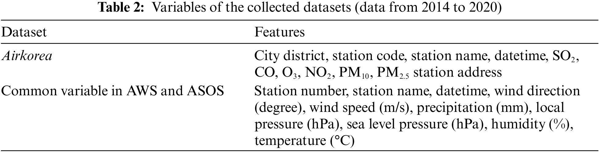
The meteorological dataset comprises information measured at two types of meteorological observatories: automated synoptic observation system (ASOS) and automatic weather system (AWS). Although the number of meteorological information measurements differed between the two observatories, data were used from both because they collected the same types of meteorological information required for this study. These two observatory systems are automated surface observation systems managed by the Meteorological Administration (KMA) in Korea. They mainly provide observations and predictions for a range of meteorological information, including wind [27], temperature, relative humidity, pressure, and precipitation at each site every minute [28]. Total 37 M samples from 630 stations (both from AWS and ASOS) from January 01, 2014, to December 31, 2020 were collected (Table 2).

In the Airkorea dataset, PM2.5, an hourly ultra fine dust concentration was recorded in 2015, and with higher level of accuracy from 2019. The observations were not stable until 2018, where the average missing ratio of the collected information from 2014 to 2018 was higher than 50%. Thus, PM10, an hourly fine dust concentration that was stably observed throughout the period, was set as the target variable instead of PM2.5.

Fig. 1 shows the distribution of observatories. The distribution of air pollutant observatories provided by AirKorea and observatories observing meteorological datasets differed as follows. Contrary to the meteorological stations, it can be confirmed that air pollutant observatories in South Korea are more concentrated in metropolitan and megalopolis areas (e.g., Seoul and Busan).

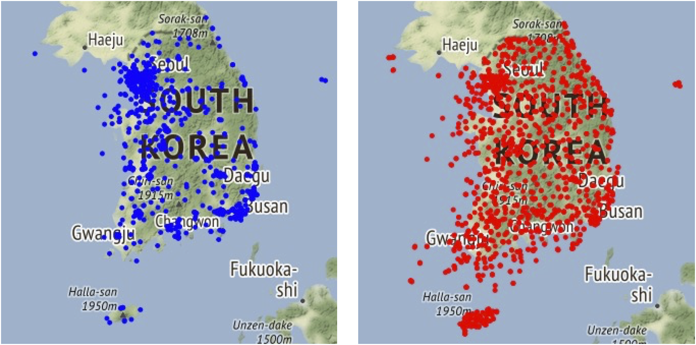
Figure 1: (Left) Air quality observatory locations, (Right) the locations of the weather observatories

2.2 Preprocessing

2.2.1 Acquisition of Location Variable

To utilize the location information, the authors first collected and added the latitude and longitude information of stations in each dataset. For the Airkorea dataset, the latitude and longitude corresponding to each station address were obtained using the Google Maps application programming interface [29]. To obtain weather information, this paper integrated the ASOS and AWS datasets into a single meteorological dataset. Additionally, the latitude and longitude information of the stations were collected and paired by utilizing the metadata provided from the KMA website. This allowed for the association of location coordinates with the corresponding air observation stations.

2.2.2 Data Merging

After pairing the latitude and longitude values of all stations in each dataset, this paper mapped the AirKorea dataset and meteorological dataset based on the shortest distance between the latitude and longitude values of each station. Specifically, the information from a meteorological station was mapped to the nearest AirKorea station based on its locational and seasonal information. A library called haversine [30] in Python was used to calculate the distance between the two stations. This method is utilized to compute the distance between two points along a great circle, which represents the shortest path over the Earth’s surface. The calculation was done using the following formulas [30]:

θ=dr(2)

hav(θ)=sin2(θ2)=h(3)

d=2r × arcsin(h)(4)

Notably, in formula (4), d signifies the distance between two points along the great circle of a sphere, with r representing the sphere’s radius [30]. This article can obtain the value d through the haversine function 3. In the context of a sphere, θ represents the central angle formed between any two points [30], while formula (2) shows how to calculate it. Finally, the locationally proximate meteorological stations were mapped based on the hourly date and time with the Airkorea dataset.

2.2.3 Handling Missing Value

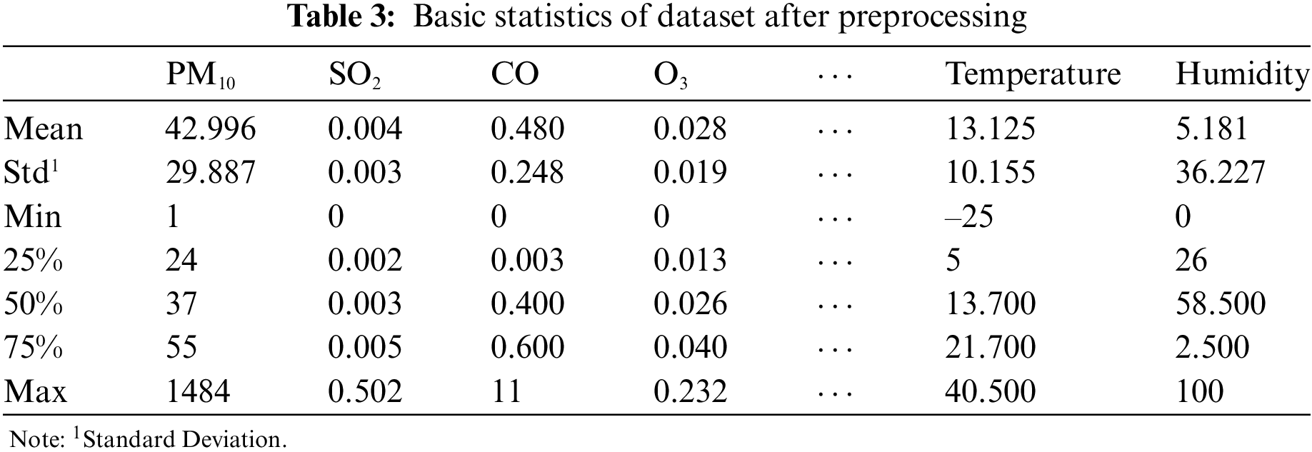
To handle missing values, any features that had more than 50% missing values were removed from the analysis. For the remaining features, a linear interpolation method was implemented using the interpolate function from the pandas library. This approach was chosen because filling null values with a single value, such as mean or median, may not be appropriate for the dataset, which consists of hourly information and exhibits clear time series characteristics. Linear interpolation, on the other hand, is more suitable for time series data as it imputes missing values based on a linear computation, taking into account the hourly fluctuations in the data. Several studies have utilized the linear interpolation method and have validated its effectiveness compared to other methods, such as single interpolation [31,32]. Moreover, this paper eliminated samples with zero PM10. Table 3 shows the basic statistics after the overall preprocessing.

2.3 Feature Selections

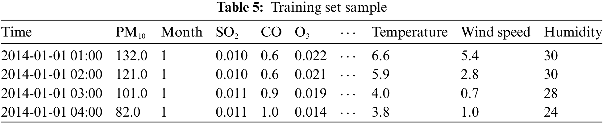
For feature selection, this paper calculated the correlation coefficients, and features with an absolute correlation coefficient greater than 0.1 were selected as the final variables. Even if the correlation was lower than the standard, variables found to be important in previous studies were also considered [33,34]. Finally, the month was separated from datetime and added as a variable. The final selected variables are presented in Table 4. Fig. 2 and Table 5 show their correlation coefficient with PM10 and an example of our training dataset, respectively.

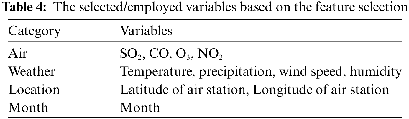
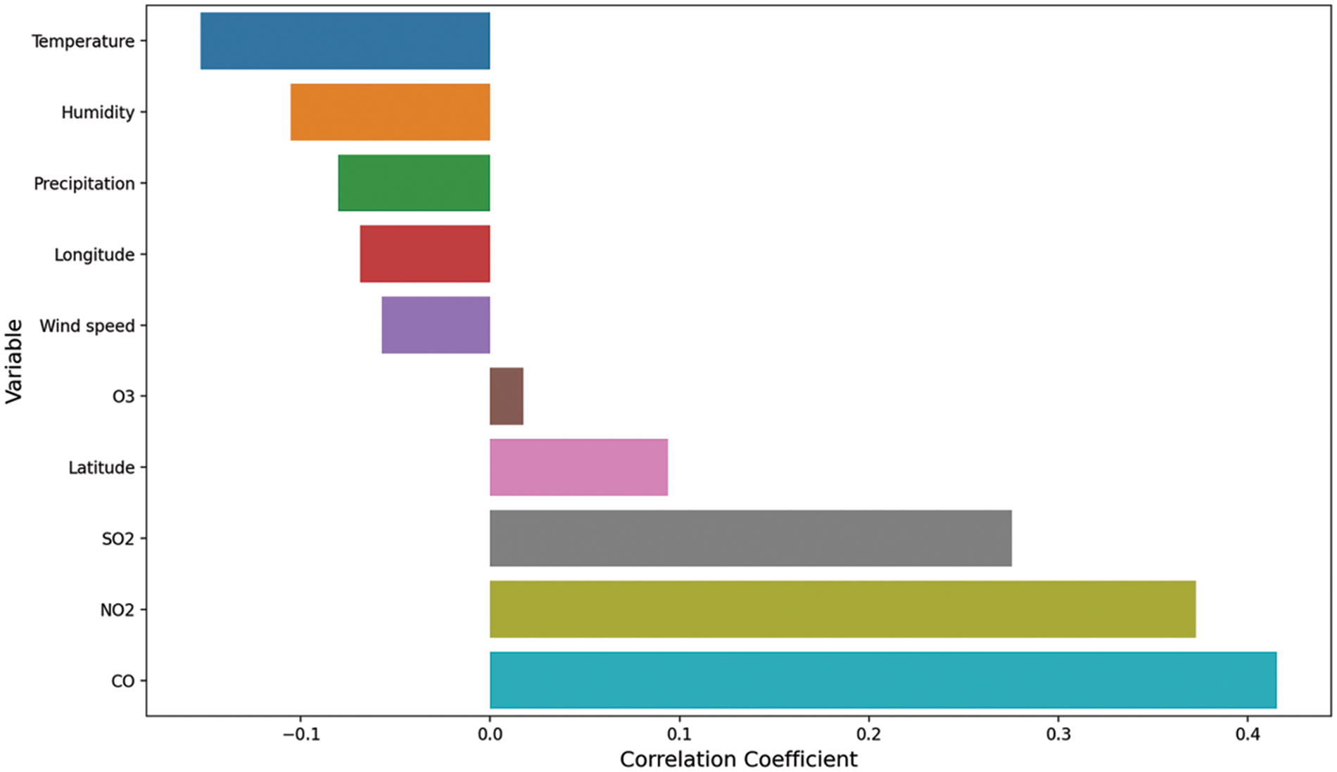
Figure 2: Correlation coefficient with PM10

2.4 Predictive Algorithms

RF regression (RFR), XGBoost regression (XGB), AdaBoost regression (Ada), and LSTM models were used to predict PM10 levels. RFR is a supervised machine learning algorithm for numeric variable prediction. It is an ensemble algorithm that combines multiple models for higher accuracy of prediction results. Results of multiple decision trees are joined, and the mean of each decision tree is the output.

The RFR model used in this study is robust against overfitting due to its implementation of a bootstrapping method during the construction of individual trees. This technique helps to reduce the risk of overfitting by randomly sampling the training data for each tree. However, note that the RFR model can be memory intensive due to the aggregation process of the individual trees. The process of combining the predictions from multiple trees requires additional memory resources.

XBG is a boosting method for an ensemble algorithm. This method sequentially applies a decision tree and the error of the previous model is considered as the weight of the next model. A calculated value reflecting the weights of all steps is the final result of the boosting. XGB is a representative model of the boosting method and XGB regression is used for numeric value prediction. XGB would be computationally intensive because it is an ensemble algorithm, while feature importance could be obtained through this model. Ada is an adaptive boosting method. Although the basic Ada algorithm is the same as XGB, it applies different weights to individual weak classifiers. Ada is vulnerable to biased dataset, while it is robust to imbalanced dataset and could deal with it easily. Last, LSTM is the recurrent neural network (RNN) model used for dealing with sequential data and its core is a memory cell that remembers the results from the previous hidden layer. RNN model performs the task through a recursive use of information, which means in each time step (t), output of the previous time step (t−1) memory cell is used as input. The problem of RNN model is long term dependency, a phenomenon where the values of the distant past hidden layers are not transmitted to the end. The concept of LSTM was introduced to ameliorate the problem of long-term dependency [35]. To solve the above problem, LSTM utilized forget (ft), input (it), and output (ot) gates. The structure of the LSTM cell is presented in Fig. 3. The forget gate decides the type of information to be abandoned from the previous cell. The input gate decides what to store in the current cell among the new information input. In the update process, the old cell state (Ct−1) is computed and reflected to the new cell state (Ct). The output gate determines the output value. LSTM is an appropriate method to sequential dataset, but it is such a ‘black-box’ model. This point indicates that the influence of features and results cannot be interpreted. In this research, two different variable sets were used. First, “Air + Weather” set is composed of pollutant and meteorological information. Second, “ALL” set is composed of all pollutant, meteorological and location information.

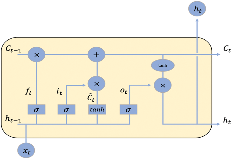
Figure 3: LSTM cell structure

2.5 Evaluation Metrics

Each model was evaluated using five metrics: Mean Squared Error (MSE), Root Mean Squared Error (RMSE), Mean Absolute Error (MAE), Mean Absolute Percentage Error (MAPE), and Pearson Correlation. MSE (formula (5)) represents the average difference between the actual and predicted values. A lower MSE indicates higher accuracy of the regression model. RMSE (formula (6)) is the square root of mean squared error (MSE) which mitigates the distortion resulting from MSE [36]. MAE (formula (7)) is the mean of the absolute variances between the observed and estimated values [36]. A lower MAE indicates better model performance. This metric is intuitive but can be influenced by the scale of the data. MAPE (formula (8)) improves the scale-dependency issue of MAE by expressing it as a percentage. It provides an assessment of the mean percentage deviation between the observed and estimated values [37]. Pearson Correlation (formula (9)) is used as a metric for evaluating the level of similarity between the observed and estimated values [38]. It measures the linear relationship between two variables and indicates how well the predicted values align with the actual values.

MSE=1n∑i=1n[Yi−Yi^]2(5)

RMSE=1n∑i=1n[Yi−Yi^]2(6)

MAE=1n∑i=1n|Yi−Yi^|(7)

MAPE=100n∑i=1n|Yi−Yi^Yi|(8)

R=∑i=1n(Yi−Y)×(Y^i−Y^)∑i=1n(Yi−Y)2×∑i=1n(Y^i−Y^)2(9)

2.6 Modeling Approach

For the input features of RFR, XGB, and Ada, the integrated and validated datasets of 574 stations were split into training (394 stations, 70%), validation (50 stations, 10%), and testing (94 stations, 20%) datasets, respectively. Training set is composed of 15,434,716 rows and 11 columns. Validation set is composed of 1,975,360 rows and 11 columns. Lastly, the test set is composed of 3,572,464 rows and 11 columns. For the input features of LSTM, which utilizes the sequential characteristics of input features, this paper shifted the variables 5 h before the time of the targeted PM10. Fig. 4 presents an overview of the shifted procedures. Training set is composed of 15,433,140 rows and 51 columns. Validation set is composed of 1,975,160 rows and 51 columns. Lastly, the test set is composed of 3,572,088 rows and 51 columns.

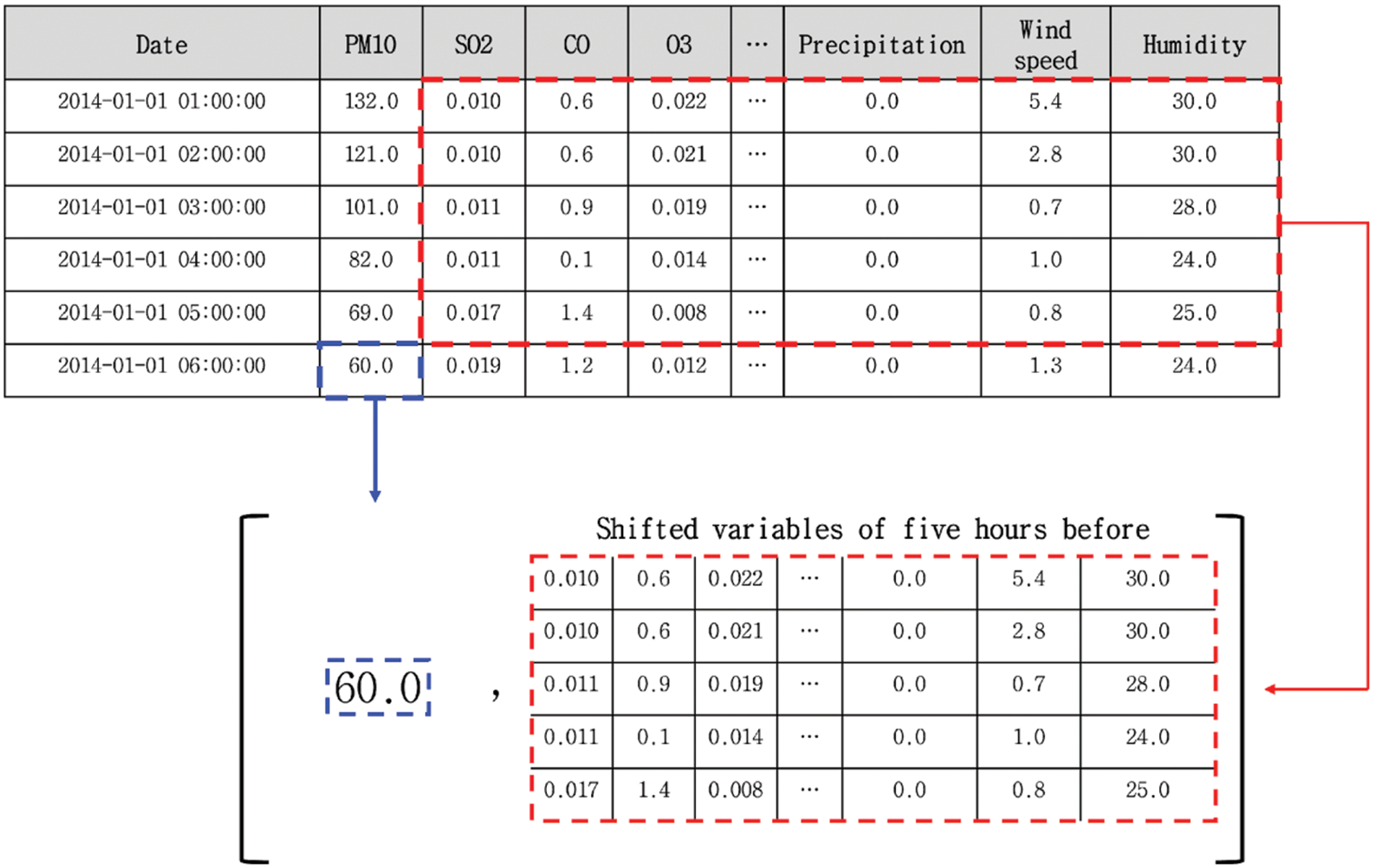
Figure 4: Example of data shifting

We set the number of estimators as 100, minimum of samples to split as 2, randomness of bootstrapping as 42 and number of jobs to run parallel as −1 for RFR. For XGB, number of estimators set as 100, learning rate as 0.01, minimum of split loss as 0, ratio of sampling as 0.75, ratio of feature sampling as 1 and maximum depth set as 7. For Ada, the autors set the number of estimators as 100, learning rate as 1.0 and loss function for weights as ‘linear’. The LSTM structure is presented in Fig. 5. Python 3.6 and Tensorflow 2.4 on GeForce RTX 3060 TI 8 GB GPU were employed for the experiments.

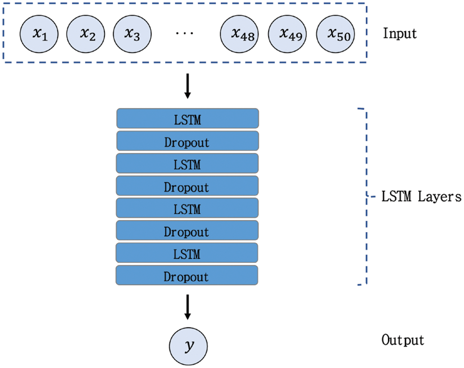
Figure 5: Overview of LSTM: All shifted data served as an input of model and propagated through several LSTM and dropout layers. Ultimately, predicted PM10 value was obtained

3  Result and Discussion

Based on the employed metrics and the findings of prior research [39–43], the RMSE and Pearson correlation are mainly considered our main metrics. Table 6 and Fig. 6 summarize the results. The study considered various pairs of input sets and compared the performance of each pair. Two pairs, namely Air + Weather and ALL, achieved better results for the machine learning models, while the LSTM model yielded the best overall performance. Fig. 7 displays the distribution of actual and predicted values for the LSTM model and indicates a significant similarity between the distributions of the actual and predicted values. Fig. 8 is a plot of PM10 values in the low range and shows the relationship between true and predicted values of LSTM. This indicates that the model can relatively well predict low-range PM10 values rather than larger values and spikes. Air-related variables such as NO2 and SO2 generally had significant importance in overall machine learning methods. In the case of the Air + Weather set, CO and SO2 acted as important variables of XGB, CO and temperature were important variables of Ada. In the All set, CO and SO2 were also selected as important variables of XGB. Important variables of Ada were Month, CO, and latitude of air observatories.

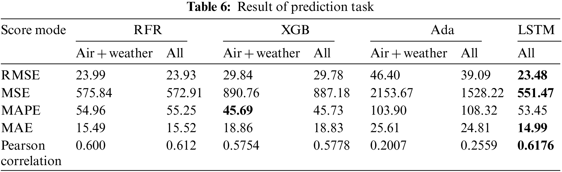
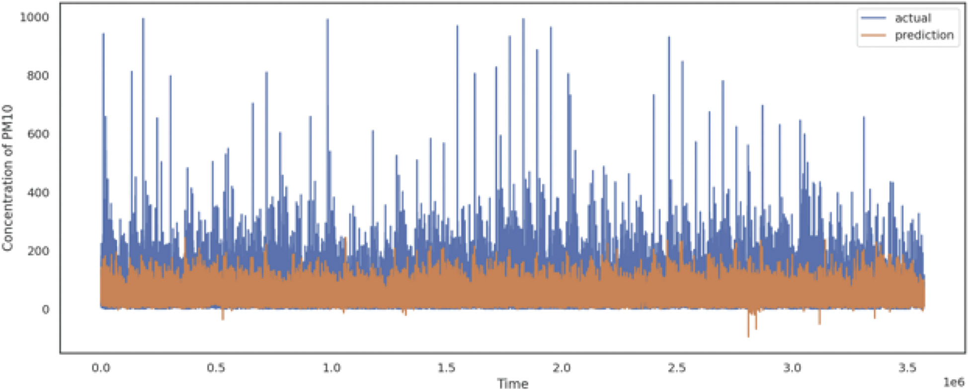
Figure 6: Prediction result of LSTM

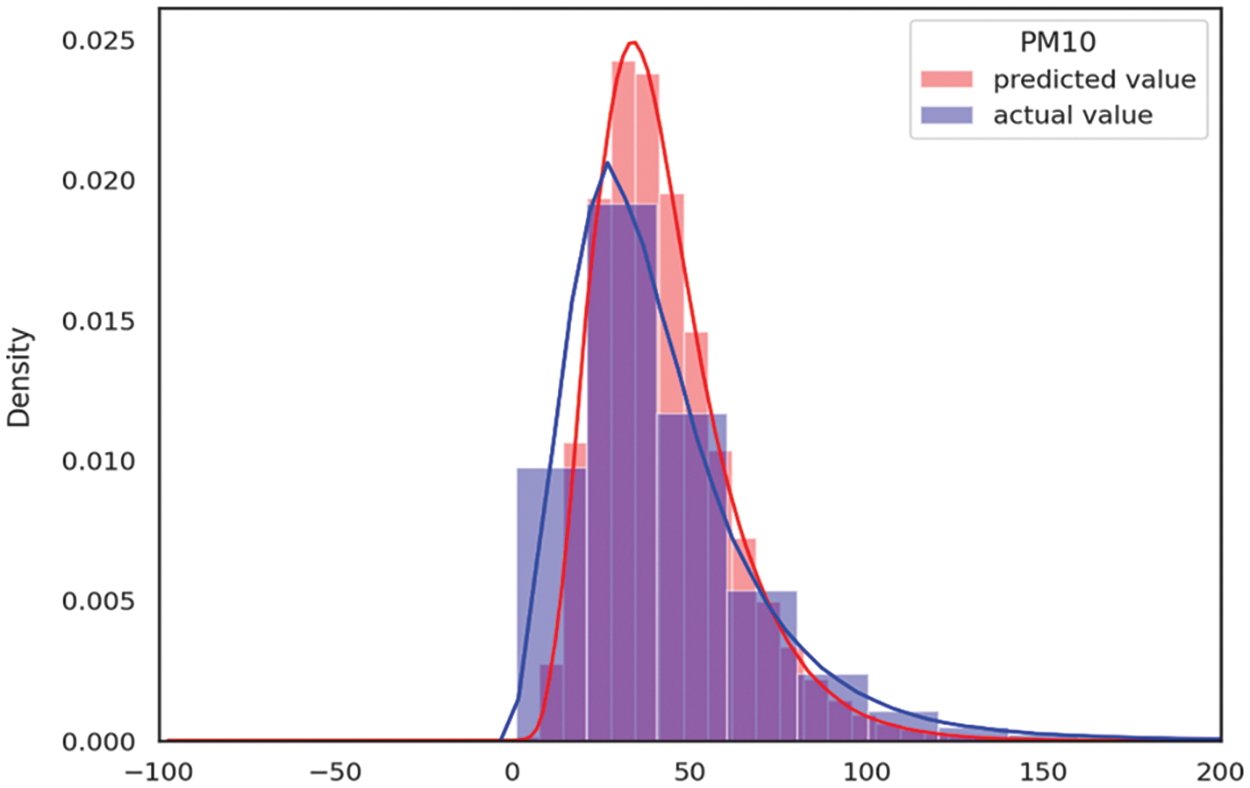
Figure 7: Distribution of actual and predicted values

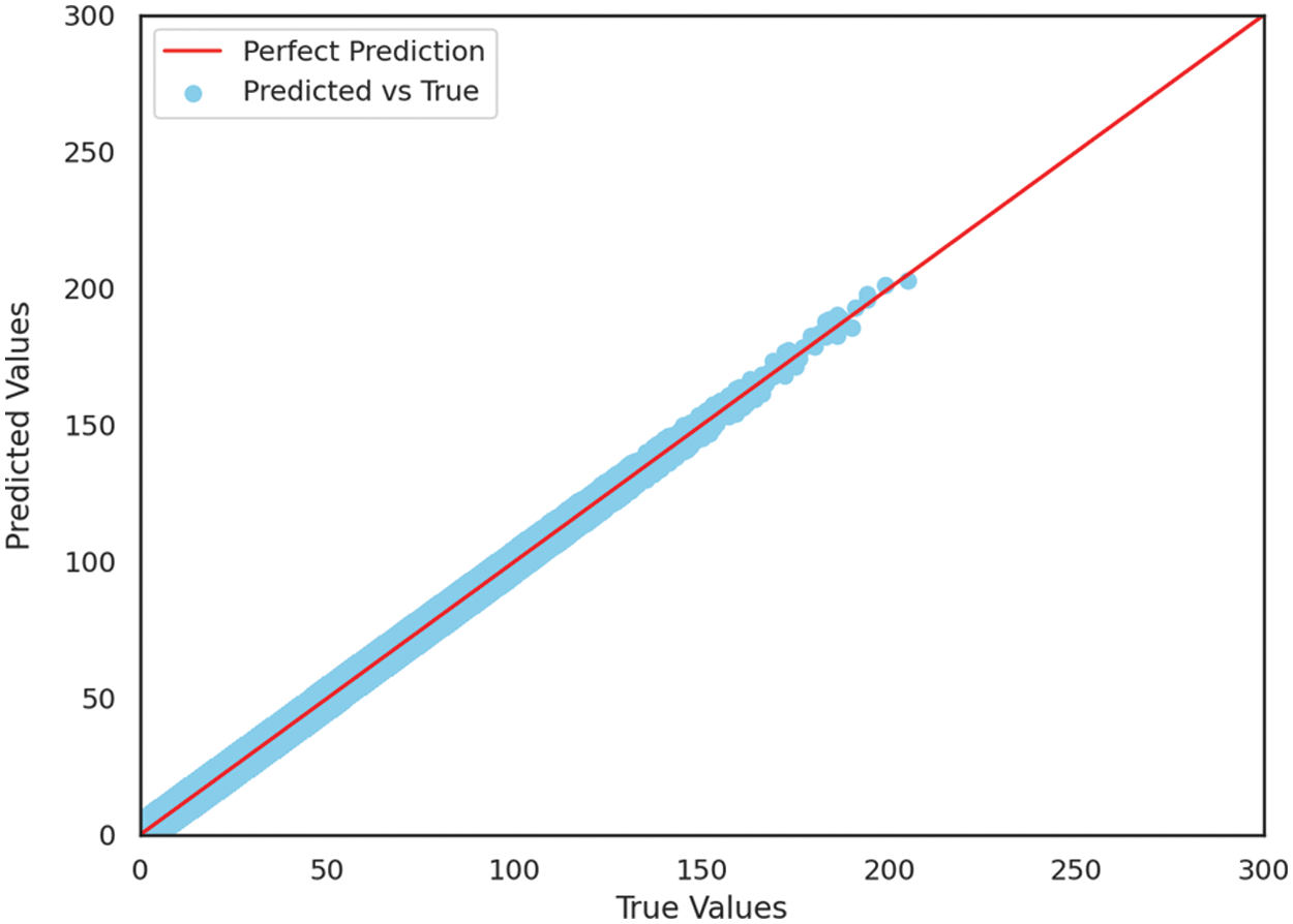
Figure 8: Scatter plot of actual and predicted values

The results revealed that LSTM performed better than all other machine learning models. The RMSE and Pearson correlation of LSTM were 23.48 and 0.6176, respectively. RFR exhibited the second-best performance, with an RMSE score and Pearson correlation of 23.93 and 0.612, respectively, slightly lower than those of LSTM. Ada and XGB exhibit inferior performance compared to LSTM due to their susceptibility to outliers and the adverse effects of noisy data. Meanwhile, LSTM exhibits greater robustness with the dataset compared to other machine learning models. The LSTM model’s superior efficacy lies in its ability to handle the temporal dynamics present in the dataset. Given the continuous temporal variations inherent in air quality and meteorological data, incorporating information from previous time steps becomes crucial for accurately predicting atmospheric conditions in subsequent time steps. The LSTM model effectively recognizes and leverages these intrinsic characteristics, resulting in better performance compared to other machine learning models that only utilize the month variable for time-related information.

Overall, the models that included all features, including location information (latitude and longitude values of each station), outperformed models that solely relied on air quality and meteorological information. In a comparative study, incorporating location information improved the performance of RFR, XGB, and Ada, with respective R of 0.612, 0.5778, and 0.2559, compared to scenarios where location information was omitted (R of 0.600, 0.5754, and 0.2007, respectively). This highlights the value of incorporating micro-location features to enhance the prediction model and achieve fine dust level predictions in areas without nearby observatories.

The results of our study can be considered satisfactory, considering the uniqueness of our dataset and the differences in variables and preprocessing methods used in previous studies. It is also noteworthy that the inclusion of local information improved model performance. Although outliers were not specifically addressed due to the nature of the dataset as a natural phenomenon and interpolation was performed to handle a significant portion of missing values, the model demonstrated good predictive performance, except for extreme spikes in PM10 values (Figs. 6 and 7). As a consequence, this article demonstrated the efficacy of micro-location mapping method for data-scarce region by achieving a certain level of performance without complicated preprocessing method, except for extreme spikes in PM10 values (Figs. 6–8). Especially, Fig. 8 represents the successfully predicted values of our LSTM model.

4  Conclusion

Our research aimed to address the prediction of fine dust levels in specific micro-locations where observatories are lacking. This article collected datasets from meteorological observatories (ASOS and AWS) and Airkorea, covering the period from January 2014 to December 2020. The air dataset consisted of a total of 23 million samples from 957 stations, with an average of 11 features per sample. To achieve accurate fine dust prediction, this article proposed an innovative strategy that incorporates micro-location information (latitude and longitude). The machine learning and deep learning models used for PM10 prediction included RFR, XGB, Ada, and LSTM. Evaluation of these models was conducted using standard metrics such as RMSE, MSE, MAPE, MAE, and Pearson correlation. The results demonstrated an intensive correlation between the true and predicted values, validating the effectiveness of our approach. This paper particularly highlighted the significance of incorporating latitude and longitude variables, which significantly improved prediction accuracy. Among the models, LSTM performed the best by capturing temporal dependencies across distant time steps, achieving a Pearson correlation of 0.6176.

This study holds significant implications for both scholarly and practical aspects. By incorporating micro-location values and utilizing a time-series dataset, this paper enhances the understanding of factors influencing PM10 levels and improve prediction accuracy, contributing to the existing knowledge base. Moreover, our research emphasizes the importance of alternative approaches in data-scarce regions, enhancing environmental monitoring and addressing regional disparities. In practical terms, our approach contributes to public health management by providing accurate information for informed decision-making and targeted interventions, ensuring equal access to information in rural areas without observation systems. Furthermore, the use of micro-location information enables a localized and effective approach to tackle air pollution concerns, optimize resource allocation, and mitigate the impacts of fine dust pollution more effectively.

However, our study also has some limitations. Firstly, there is a trade-off between interpolating missing values and removing them in the meteorological observation data. While this paper employed linear interpolation, the interpolated values may not fully represent the actual data and could introduce potential distortions and inaccuracies. On the other hand, removing missing values ensures data accuracy and enhances the reliability of analysis results but may result in information loss. Future research could explore the performance comparison between interpolated data and data with missing values completely removed, considering the implications of each approach. Secondly, additional diverse data pre-processing procedures could be explored in future studies. Apart from the methodology employed in this study, the inclusion of various scaling techniques, the generation of derived variables, and the incorporation of data from other modalities related to weather observation, such as satellite photos, could be considered.

Acknowledgement: S. Kim and H. Yu are equally contributed first authors.

Funding Statement: This research was supported by the MSIT (Ministry of Science and ICT), Korea, under the ICAN (ICT Challenge and Advanced Network of HRD) Program (IITP-2020-0-01816) supervised by the IITP (Institute of Information & Communications Technology Planning & Evaluation). This research was also supported by National Research Foundation (NRF) of Korea Grant funded by the Korean Government (MSIT) (No. 2021R1A4A3022102).

Author Contributions: Study conception and design: S. Kim, H. Yu, E. Park; data collection: S. Kim, H. Yu; analysis and interpretation of results: S. Kim, H. Yu, J. Yoon; draft manuscript preparation:S. Kim, H. Yu, J. Yoon, E. Park. All authors reviewed the results and approved the final version of the manuscript.

Availability of Data and Materials: The data that support the findings of this study are openly available in Github at https://github.com/dxlabskku/FineDust.

Conflicts of Interest: The authors declare that they have no conflicts of interest to report regarding the present study.

References

1. J. Czerwinska and G. Wielgosinski, “The effect of selected meteorological factors on the process of “polish smog” formation,” Journal of Ecological Engineering, vol. 21, no. 1, pp. 180–187, 2020. [Google Scholar]

2. P. M. Mannucci and M. Franchini, “Health effects of ambient air pollution in developing countries,” International Journal of Environmental Research and Public Health, vol. 14, no. 9, pp. 1048, 2017. [Google Scholar] [PubMed]

3. Y. Hassoun, C. James and D. I. Bernstein, “The effects of air pollution on the development of atopic disease,” Clinical Reviews in Allergy & Immunology, vol. 57, no. 3, pp. 403–414, 2019. [Google Scholar]

4. M. Kampa and E. Castanas, “Human health effects of air pollution,” Environmental Pollution, vol. 151, no. 2, pp. 362–367, 2008. [Google Scholar] [PubMed]

5. Y. Wang, K. Sun, L. Li, Y. Lei, S. Wu et al., “The impacts of economic level and air pollution on public health at the micro and macro level,” Journal of Cleaner Production, vol. 366, pp. 132932, 2022. [Google Scholar]

6. H. Park, M. Byun, T. Kim, J. J. Kim, J. S. Ryu et al., “The washing effect of precipitation on PM10 in the atmosphere and rainwater quality based on rainfall intensity,” Korean Journal of Remote Sensing, vol. 36, no. 63, pp. 1669–1679, 2020. [Google Scholar]

7. K. H. Kim, E. Kabir and S. Kabir, “A review on the human health impact of airborne particulate matter,” Environment International, vol. 74, pp. 136–143, 2015. [Google Scholar] [PubMed]

8. J. D. Sacks, L. W. Stanek, T. J. Luben, D. O. Johns, B. J. Buckley et al., “Particulate matter–induced health effects: Who is susceptible?,” Environmental Health Perspectives, vol. 119, no. 4, pp. 446–454, 2011. [Google Scholar] [PubMed]

9. K. Mortimer, L. Neas, D. Dockery, S. Redline and I. Tager, “The effect of air pollution on inner-city children with asthma,” European Respiratory Journal, vol. 19, no. 4, pp. 699–705, 2002. [Google Scholar] [PubMed]

10. H. Kim and T. Moon, “Machine learning-based fine dust prediction model using meteorological data and fine dust data,” Journal of the Korean Association of Geographic Information Studies, vol. 24, no. 1, pp. 92–111, 2021. [Google Scholar]

11. D. Y. Jeong, “Socio-economic costs from yellow dust damages in South Korea,” Korean Social Science Journal, vol. 35, no. 2, pp. 1–29, 2008. [Google Scholar]

12. P. Srinamphon, S. Chernbumroong and K. Y. Tippayawong, “The effect of small particulate matter on tourism and related smes in Chiang Mai, Thailand,” Sustainability, vol. 14, no. 13, pp. 8147, 2022. [Google Scholar]

13. M. Gao, S. K. Guttikunda, G. R. Carmichael, Y. Wang, Z. Liu et al., “Health impacts and economic losses assessment of the 2013 severe haze event in Beijing area,” Science of the Total Environment, vol. 511, pp. 553–561, 2015. [Google Scholar] [PubMed]

14. D. Kang and J. E. Kim, “Fine, ultrafine, and yellow dust: Emerging health problems in Korea,” Journal of Korean Medical Science, vol. 29, no. 5, pp. 621–622, 2014. [Google Scholar] [PubMed]

15. E. Adamiec, J. Dajda, A. Gruszecka-Kosowska, E. Helios-Rybicka, M. Kisiel-Dorohinicki et al., “Using mediumcost sensors to estimate air quality in remote locations. Case study of Niedzica, Southern Poland,” Atmosphere, vol. 10, no. 7, pp. 393, 2019. [Google Scholar]

16. National Institute of Environmental Research, Air Pollution Monitoring Network Installation and Operation Guidelines, 2021. [Online]. Available: https://www.airkorea.or.kr/web/ [Google Scholar]

17. Y. Yu, J. Kim and D. Jeong, “Design of a portable sensor data sharing system for measuring particular matter,” in Proc. of KIIT Conf., Gumi, Korea, pp. 424–426, 2017. [Google Scholar]

18. T. Yang, H. Cho, S. Kim, C. Kim and S. H. Kim, “Improvement of reliability of air quality service using low-cost equipment,” in Proc. of the Korean Institute of Communication Sciences Conf., Jeju, Korea, pp. 1122–1123, 2019. [Google Scholar]

19. S. H. Kim, J. Jeong, M. Hwang and C. Kang, “Development of an IoT-based atmospheric environment measurement and analysis system,” The Journal of the Korean Institute of Communications and Information Sciences, vol. 43, no. 9, pp. 1750–1764, 2017. [Google Scholar]

20. X. Ni, H. Huang and W. Du, “Relevance analysis and short-term prediction of PM2.5 concentrations in Beijing based on multi-source data,” Atmospheric Environment, vol. 150, pp. 146–161, 2017. [Google Scholar]

21. K. P. Singh, S. Gupta, A. Kumar and S. P. Shukla, “Linear and nonlinear modeling approaches for urban air quality prediction,” Science of the Total Environment, vol. 426, pp. 244–255, 2012. [Google Scholar] [PubMed]

22. S. Kim, J. M. Lee, J. Lee and J. Seo, “Deep-dust: Predicting concentrations of fine dust in Seoul using LSTM,” in Proc. of the 8th Int. Workshop on Climate Informatics, Boulder, Colorado, USA, pp. 34–36, 2018. [Google Scholar]

23. S. Jeon and Y. S. Son, “Prediction of fine dust PM10 using a deep neural network model,” The Korean Journal of Applied Statistics, vol. 31, no. 2, pp. 265–285, 2018. [Google Scholar]

24. S. Kim, K. H. Hong, H. Jun, Y. J. Park, M. Park et al., “Effect of precipitation on air pollutant concentration in Seoul, Korea,” Asian Journal of Atmospheric Environment, vol. 8, no. 4, pp. 202–211, 2014. [Google Scholar]

25. H. J. Chae, “Effect on the PM10 concentration by wind velocity and wind direction,” Journal of Environmental and Sanitary Engineering, vol. 24, no. 3, pp. 37–54, 2009. [Google Scholar]

26. AirKorea, Status of Air Observation System, 2005. [Online]. Available: https://www.airkorea.or.kr/web/contents/contentView/ [Google Scholar]

27. I. Noh, H. W. Doh, S. O. Kim, S. H. Kim, S. Shin et al., “Machine learning-based hourly frost-prediction system optimized for orchards using automatic weather station and digital camera image data,” Atmosphere, vol. 12, no. 7, pp. 846, 2021. [Google Scholar]

28. B. Y. Kim, J. W. Cha, K. H. Chang and C. Lee, “Visibility prediction over South Korea based on random forest,” Atmosphere, vol. 12, no. 5, pp. 552, 2021. [Google Scholar]

29. Google, Google Maps Platform, 2005. [Online]. Available: https://console.cloud.google.com/google/maps-apis/overview/ [Google Scholar]

30. Python, Haversine 2.6.0, 2018. [Online]. Available: https://pypi.org/project/haversine/ [Google Scholar]

31. N. M. Noor, M. M. Al Bakri Abdullah, A. S. Yahaya and N. A. Ramli, “Comparison of linear interpolation method and mean method to replace the missing values in environmental data set,” Materials Science Forum, vol. 803, pp. 278–281, 2015. [Google Scholar]

32. M. N. Norazian, Y. A. Shukri, R. N. Azam and A. M. M. Al Bakri, “Estimation of missing values in air pollution data using single imputation techniques,” ScienceAsia, vol. 34, no. 3, pp. 341–345, 2008. [Google Scholar]

33. T. Nishanth, K. Praseed, M. S. Kumar and K. Valsaraj, “Influence of ozone precursors and PM10 on the variation of surface O3 over Kannur, India,” Atmospheric Research, vol. 138, pp. 112–124, 2014. [Google Scholar]

34. A. di Ciaula and M. Bilancia, “Relationships between mild PM10 and ozone urban air levels and spontaneous abortion: Clues for primary prevention,” International Journal of Environmental Health Research, vol. 25, no. 6, pp. 640–655, 2015. [Google Scholar] [PubMed]

35. S. Hochreiter and J. Schmidhuber, “Long short-term memory,” Neural Computation, vol. 9, no. 8, pp. 1735–1780, 1997. [Google Scholar] [PubMed]

36. S. Hwang, H. Ahn and E. Park, “iMovieRec: A hybrid movie recommendation method based on a user-image-item model,” International Journal of Machine Learning and Cybernetics, vol. 14, pp. 1–12, 2023. [Google Scholar]

37. J. Ko, J. Yoon, D. Choi, E. Park, S. Pack et al., “Trafficformer: A transformer-based traffic predictor,” in Proc. of the 2022 IEEE Int. Conf. on Consumer Electronics, New York, NY, USA, IEEE, pp. 1–2, 2022. [Google Scholar]

38. S. Hwang and E. Park, “Movie recommendation systems using actor-based matrix computations in South Korea,” IEEE Transactions on Computational Social Systems, vol. 9, no. 5, pp. 1387–1393, 2022. [Google Scholar]

39. X. Song, J. Huang and D. Song, “Air quality prediction based on LSTM-kalman model,” in Proc. of Information Technology and Artificial Intelligence Conf. (ITAIC), New York, NY, USA, pp. 695–699, 2019. [Google Scholar]

40. H. Zhang, G. Chen, J. Hu, S. H. Chen, C. Wiedinmyer et al., “Evaluation of a seven-year air quality simulation using the Weather Research and Forecasting (WRF)/Community Multiscale Air Quality (CMAQ) models in the Eastern United States,” Science of the Total Environment, vol. 473, pp. 275–285, 2014. [Google Scholar] [PubMed]

41. W. Wei, O. Ramalho, L. Malingre, S. Sivanantham, J. C. Little et al., “Machine learning and statistical models for predicting indoor air quality,” Indoor Air, vol. 29, no. 5, pp. 704–726, 2019. [Google Scholar] [PubMed]

42. G. K. Kang, J. Z. Gao, S. Chiao, S. Lu and G. Xie, “Air quality prediction: Big data and machine learning approaches,” International Journal of Environmental Science and Development, vol. 9, no. 1, pp. 8–16, 2018. [Google Scholar]

43. K. Siwek and S. Osowski, “Data mining methods for prediction of air pollution,” International Journal of Applied Mathematics and Computer Science, vol. 26, no. 2, pp. 467–478, 2016. [Google Scholar]