
 Submit a Paper
 Propose a Special lssue
 Open Access
ARTICLE
Research on the Change of Airfoil Geometric Parameters of Horizontal Axis Wind Turbine Blades Caused by Atmospheric Icing
1 College of Mechanical and Electrical Engineering, Shihezi University, Shihezi, 832003, China
2 Beijing Goldwind Science Creation Windpower Equipment Co., Ltd., Beijing, 100176, China
* Corresponding Author: Hui Zhang. Email:
Energy Engineering 2022, 119(6), 2549-2567. https://doi.org/10.32604/ee.2022.020854
Received 16 December 2021; Accepted 05 May 2022; Issue published 14 September 2022
 View Full Text
 Download PDF
Abstract
Icing can significantly change the geometric parameters of wind turbine blades, which in turn, can reduce the aerodynamic characteristics of the airfoil. In-depth research is conducted in this study to identify the reasons for the decline of wind power equipment performance through the icing process. An accurate experimental test method is proposed in a natural environment that examines the growth and distribution of ice formation over the airfoil profile. The mathematical models of the airfoil chord length, camber, and thickness are established in order to investigate the variation of geometric airfoil parameters under different icing states. The results show that ice accumulation varies considerably along the blade span. By environmental temperature drop, the minimum and maximum extents of ice accumulation are observed near the blade root (0.2 R) and the blade tip (0.95 R), respectively (R represents the blade length). The icing process steadily increases the chord length and decreases the airfoil curvature, reaching the largest value at the blade tip region. Furthermore, the maximum curvature is reduced to 41.50% of the original curvature. The maximum camber position of the airfoil moves towards the trailing edge, and the most prominent position occurs at the middle blade region (0.6 R), where it moves back by 19.43%. Ice accumulation steadily increases airfoil thickness. It leads to the maximum thickness growth of 53.40% that occurs at the blade tip region and moves forward to the leading edge by 10%. The research results can provide the required theoretical support for further monitoring the blades operating conditions to ensure reliable wind turbines’ operation.Keywords
Notations
| The chord length, (mm); | |
| The curvature coefficient; | |
| The thickness coefficient; | |
| The vertical distance between the lower surface of the airfoil and the chord line, (mm); | |
| The vertical distance between the upper surface and the lower surface, (mm); | |
| The measured value of icing on the lower surface of the measuring point, (mm); | |
| The measured value of icing on the upper surface of the measuring point, (mm); | |
| The different monitoring positions (i = 0.2, 0.6, 0.95); | |
| Curvature curve equation constant; | |
| Thickness curve equation constant; | |
| The value of 10 equal parts of the airfoil chord length; | |
| The number of the measuring point (n = 1, 2, 3,…, 11); | |
| The wingspan direction; | |
| R | The blade length; |
| The any length in the chord direction; | |
| The abscissa, indicating the length of the measuring point on the chord line, (mm); | |
| The camber, (mm); | |
| The ordinate, indicating the camber value of the measuring point, (mm); | |
| The thickness; | |
| The ordinate, indicating the thickness of the measuring point, (mm); | |
| The tip speed ratio of leaf element at different length ri from the root of the leaf; | |
| The twist angle of leaf element, (°); | |
| The inclination angle of leaf element, (°). |
Wind power isone of the most useful renewable energy sources in the world due to its green, clean, low-carbon, and sustainable way of electricity generation. Although wind energy resources are abundant in either elevated or cold areas, wind turbine blades are vulnerable to possible icing in cold regions [1]. The icing of wind turbine blades is a dynamic process that not only changes geometrical parameters and surface roughness of the airfoil [2] and deteriorates the airfoil’s inherent aerodynamic characteristics and adversely affects the power generation. In addition, serious icing can also cause safety problems and shutdown losses [3–5].
So far, research on wind turbine icing has mostly focused on three issues: 1. The impact of icing on power loss; 2. The effect of icing on blade vibration or deterioration of aerodynamic performance; 3. Classification of ice types and the effect of ice formation at different blade positions on the output power of wind turbines. Based on the literature, icing deteriorates the aerodynamic performance of the blades, which in turn decreases wind turbine output. An in-depth analysis of the principal reasons for such degradation is scarce, and it is necessary to study the influence of icing on the geometrical parameters of the airfoil.
The performance of wind turbine blades is considerably affected by different ice types and thicknesses over the blade surface. To examine the impact of the icing environment on the wind turbine airfoil parameters, it is necessary to study the dynamic process of blade icing. Some researchers have employed 2D or 3D computational fluid dynamics (CFD). They simulated airflow/droplet behavior and the resulting ice accumulation on the turbine blades [6,7]. Depending on the environmental temperature, rime and glaze ice are two types of ice forming on the wind turbine blades [8]. Liu et al. [9] stated that rime ice formation is related to low temperature (below −10°C), low liquid water content, and small median volume diameter (MVD) of water droplets. Since the water droplets almost instantaneously freeze when impacting the blade, the early rime usually forms in the vicinity of the original blade contour. Gao et al. [10] pointed out that the glaze ice causes more significant aerodynamic performance less than the rime ice. Generally, the formation of glaze ice directly corresponds to high temperature (more than −10°C), high liquid water content, and large MVD of water droplets. In comparison with the rime, it was declared in various research [11–13] that the glaze ice is the most dangerous type of icing. Because of the wet characteristics of the glaze ice, its shape is more complicated, and accurate prediction of its profile is more difficult. It forms “horn-shaped ice” and larger “feather-shaped ice” that grow outward into the airflow, which can significantly deform the blade surface. It was shown by Bragg et al. [14] that the formation of the glazed ice causes large-scale airflow separation and considerably decreases the airfoil aerodynamic performance. More specifically, it sharply increases the drag and decreases the lift forces.
Because of the extensive application of wind turbines and the rapid growth of computational resources, numerous studies have been conducted on wind turbine blade airfoils under various operating conditions. Li et al. [15] studied the aerodynamic characteristics of wind turbine blades with NACA0012 airfoil under a wind-sand environment. They examined the effect of concentration and particle size variations in such multiphase flow. Li et al. [16] numerically analyzed the effect of the airfoil angle of attack on the distribution of salt spray particles around the blade wall. They also investigated the aerodynamic characteristics of the airfoil under different salt spray concentrations. Based on airfoil icing tests by Sundaresan et al. [17], aerodynamic characteristics of the iced airfoil were decreased in comparison with those of the original clean wing configuration. Zhang et al. [18] proposed a new wind turbine airfoil based on blunt trailing-edge optimization. It could reduce the unfavorable effect of the rime ice environment on the aerodynamic characteristics. Lamraoui et al. [19] numerically explored the influence of external conditions on the performance of wind turbine blades. They concluded that the icing zone (as the cause of power loss) is located closer to the blade tip region.
The existing literature on wind turbine blade airfoil and blade icing dynamic process relies mostly on experimental research and numerical simulation. There is no study for in-depth analysis of the relation between thickness and position of icing and variation of blade airfoil parameters, however, most icing tests have been conducted based on indoor temperature control and constant speed condition, which are quite different from the icing process of real wind power equipment in a natural environment. Therefore, it is difficult to apply their research results to these engineering practices.
Applying a novel test method based on the natural environment in the present study innovation. Observation accuracy of the icing data (icing distribution over the airfoil profile) can be enhanced in a natural environment. Furthermore, this paper establishes the mathematical models for airfoil chord length, camber, and icing thickness, revealing the variation mechanism of airfoil parameters with blade icing. This paper provides the theoretical basis and technical support for further research on the airfoil optimization of wind turbine blades.
The article is organized as follows. The design of monitoring positions for airfoil icing is introduced in Section 2. The methodology is then explained in Section 3. It follows results and discussion in Section 4 and conclusions in the last section of the paper.
2 Design of Monitoring Positions of Airfoil Icing
Power generation efficiency and aerodynamic performance of a wind turbine are mainly affected by the aerodynamic characteristics of the airfoil (as an essential attribute of the blade) [20]. The airfoil geometry can be described by the following parameters, as shown in Fig. 1.
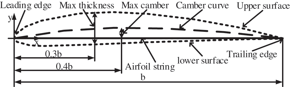
Figure 1: Geometric parameters of the airfoil
The airfoil geometry parameters mainly include leading edge, trailing edge, chord line, mid-curve, thickness, and camber [21,22]. The NACA 4412 airfoil is utilized as the blade profile in the present study. This airfoil category belongs to the low-speed airfoil series developed by the National Advisory Committee for Aeronautics (NACA), which has a higher maximum lift coefficient and a lower drag coefficient than other airfoils. The objective of the present paper is to study the icing problem of NACA 4412 airfoil by analyzing the icing impact on the geometrical parameters, including the chord length, relative thickness, and relative camber. This airfoil has a maximum relative camber of 4%, located at 40% of the chord length (as measured from the leading edge). Furthermore, the relative thickness is 12%, and the maximum thickness is located at 30% of the chord length [23]. The principal parameters of the airfoil are presented in Table 1. Fig. 2 illustrates the position of 18 sections that are considered in this study.
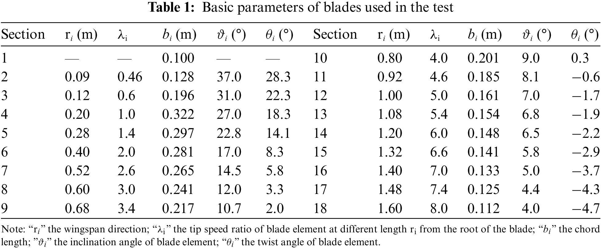
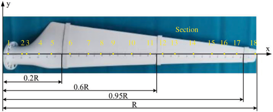
Figure 2: Blade icing monitoring position
2.2 Configuration of Ice Monitoring Points
2.2.1 Selection of Ice Monitoring Positions
Output power is an essential indicator of wind turbine performance. The influence of different blade icing positions on the nominal power of wind turbines should be examined, which requires a suitable design of ice monitoring positions. The impact of icing position on the output electricity has been investigated in the previous numerical studies. The electricity loss was mainly experienced because of blade icing alongside the span course r/R = (0.8∼0.95) [24].
Considering the above-mentioned results, therefore, he current article aims further to examine the icing drawbacks in specific blade regions. For the monitoring positions, R is the blade length, and the span routes (r/R) of 0.95, 0.6, and 0.2 are considered for the blade tip, center, and root, respectively, as shown in Fig. 2. In order to enhance the data recording accuracy at each measurement point, the NACA 4412 airfoil model is constructed using rapid prototyping technology (3D printing). It is made from aluminum alloy with low density and high rigidity to avoid uneven impeller rotation (as illustrated in Fig. 3).
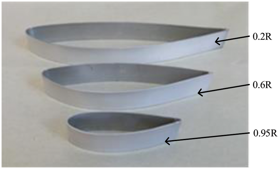
Figure 3: Airfoil model
The wall thickness of the airfoil model is 2 mm. Its surface is sprayed with the same coating material as the blade surface, and then it is wet-milled using fine (2000 grit) sandpaper to provide a smooth gloss effect of around 25 μm. Finally, a readily available all-weather protective spray enamel is applied to the polished surface. These operations are performed to reach the same surface hydrophobicity for the airfoil model and the blade and to reduce the test errors. The main parameters of the airfoil model, the chord length, and the angle of attack of the three monitoring positions are presented in Table 2.
2.2.2 Configuration of Airfoil Ice Measurement Points
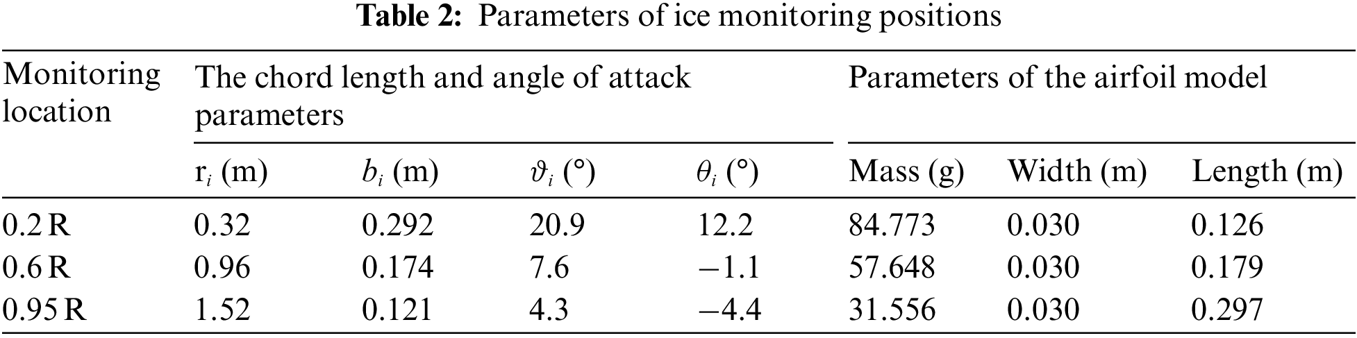
To precisely describe the impact of icing on the geometric parameters of the airfoil; the chord length is divided into ten intervals along the airfoil chord. This is performed by considering a vertical line at each dividing point and specifying the intersections of this vertical line by the upper and lower surfaces of the airfoil. These intersection points are considered the airfoil ice measurement points, including the maximum curvature and thickness positions, as demonstrated in Fig. 4.
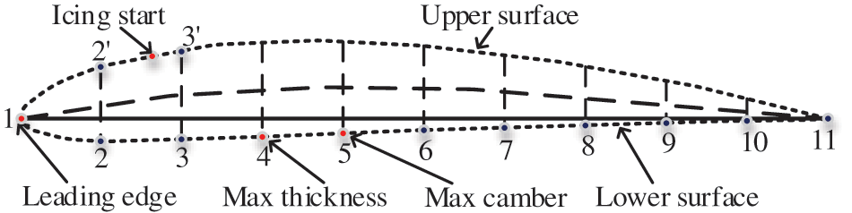
Figure 4: Configuration of airfoil ice measurement points
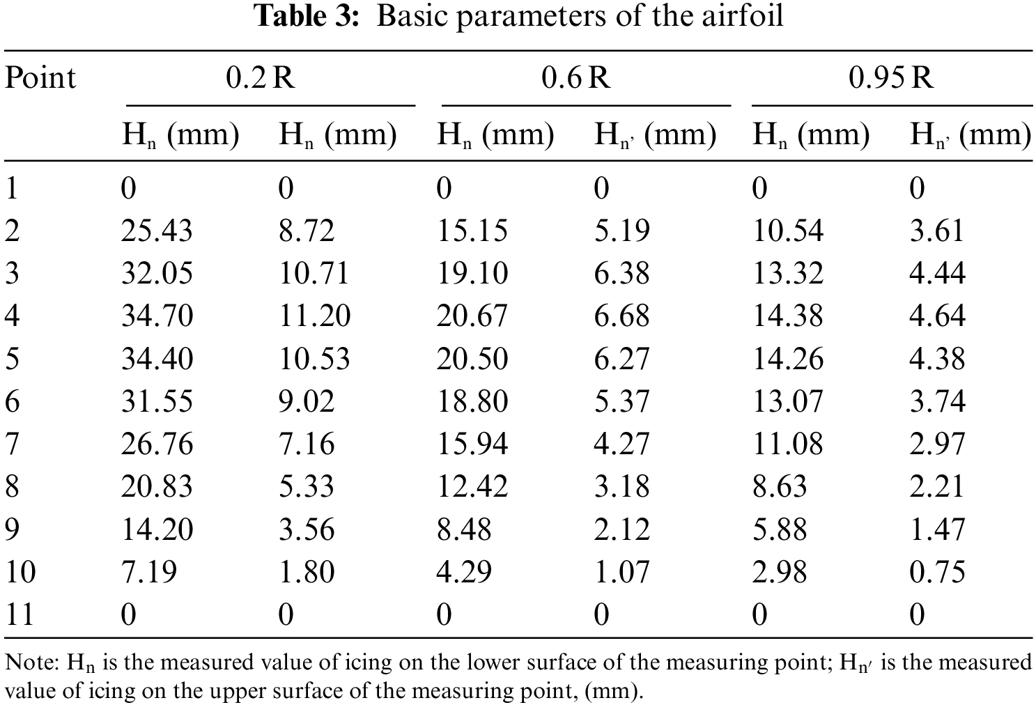
During the test, the lower surface of the blade was completely covered by ice, while the ice on the upper surface was accumulated around the main blade facet. Therefore, the intersection of vertical lines with the lower airfoil surface provides an adequate configuration for the ice measurement points n (n = 1, 2, 3, …, 11). Table 3 presents the values of Hn (vertical distance between the upper and lower surfaces) and Hn’ (vertical distance between the lower surface and the chord line) for 11 selected measurement points. The measurement points corresponding to the upper surface are notified as n’ (Fig. 4). The location of ice origination on the upper surface varies in time, such that it moves towards the trailing edge as the freezing progresses. The measurement point 1, located at the leading edge, experiences the maximum ice thickness. The measurement points 4 and 5 correspond to the maximum thickness and camber of the NACA 4412 airfoil, respectively. Therefore, these calibration points are used to measure the maximum thickness and camber, as illustrated in Fig. 4.
3.1 Wind Turbine Icing Test Device
The schematic diagram of the wind turbine blade icing test is illustrated in Fig. 5. The icing test device comprises three parts, namely a wind turbine, axial flow fan, and droplet atomization nozzle. The constructed airfoil models are initially mounted at three predetermined positions, and counterweights are installed on the remaining blades to balance their rotational inertia. At the ice thickness step, it is necessary to completely remove the airfoil model with ice attached to the blade (the icing on the airfoil model cannot be destroyed).
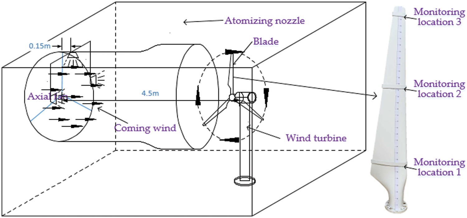
Figure 5: Schematic diagram of the icing test device
The operating parameters of the axial flow fan include the area of 1.380 mm × 1.300 m, the rated voltage of 380 V, the power rating of 1.1 kW, the air volumetric flow rate of 45,000 m3/h, and the adjustable wind speed range of 0 to 17 m/s. The cut-in wind velocity of the wind turbine is 1.5 m/s, and a three-phase permanent magnet synchronous motor is employed in the test. The wind turbine blade size is R = 1.6 m, as shown in Fig. 5, and the blade chord length is considered in the range of 0.098∼0.322 m. The water droplet atomization device comprises three atomization nozzles and a water pump. The basic parameters of the water pump include the rated power of 15 W, the rated pressure of 0.6 MPa, and the flow rate of 1.5 L/min, while for the atomization nozzle, atomizing cone angle and diameter are 120° and 0.9 m, respectively.
The blade length of the NACA 4412 airfoil is R = 1.6 m. Precise temperature and humidity meters are used to measure environmental parameters. The axial flow fan blows the water droplets (produced by the atomization device) towards the wind turbine and causes icing of the blades. About the method to capture droplets, during the test, the glass panels were placed in front of wind turbine blades; the water droplets will adhere to them. The captured water droplets are photographed under a microscope. The particle size of the water droplets is calculated according to the picture’s proportional scale, and the measured droplet diameter is converted to MVD [25]. Their diameter is calculated based on the MVD of 100 droplets to be about 20 μm. The liquid water content (LWC) in the atmosphere can be adjusted by managing the number of nozzles. LWC is measured as 0.92/g⋅m−3 by the rotating conductor monitoring method [26]. The specific parameters of the test program are summarized in Table 4.
3.3 Method of Ice Thickness Measurement
The ice thickness should be measured at the designed airfoil measurement points. However, accurate measurement of the thickness on the curved profile of the airfoil is difficult. To record more accurate data at each measurement point, before the test, the airfoil model (as shown in Fig. 3) was installed at 0.95, 0.6, and 0.2 R of the blades. The airfoil model (with the blades 0.95, 0.6, and 0.2 R) is removed after each icing test, and it is mounted on a predesigned thickness measuring device. The ultrasonic thickness measuring instrument GM100 is used to measure the icing thickness. The measurement error is ±(1%H + 0.1) mm (H is the actual thickness value), and the measurement range is 1.2–225 mm, but in some cases, it is also possible to measure smaller thicknesses with special techniques. The instrument has the function of real-time temperature compensation, which can eliminate the measurement error caused by the temperature change of the probe. The thickness of coated ice, less than 1.2 mm, is measured. Firstly, the ice is stripped from the surface of the wind turbine blade; when overlapping this ice in the same position, place it horizontally at low temperature, and impose weighs (which cannot crush the ice) on its surface, the overlapped ice will be integrated after being placed for 24 h with no cracks between the ice. And then use the ultrasonic thickness gauge to measure it. Finally, the thickness of single layer ice can be calculated.
The measurements are repeated to reduce errors and uncertainties of the test process. The employed test procedure is as follows: (1) the experiments of each group are repeated for three times and the results are recorded separately; (2) seven measurements are conducted at each point; (3) collecting and recording of the icing situation for the airfoil model. For the second step, the maximum and minimum measured data are excluded, and average of the remaining five data is regarded as the icing thickness corresponding to the target point.
In the experiments, the airfoil icing evolution is monitored by controlling time (t) and wind velocity (v). Evaluation and exposition of the results are performed for icing measurements at v = 6 m/s and t = 30, 60, 90, 120, 150 min. Table 5 presents the recorded data for 3 particular measurement points (point 1 at the airfoil leading edge, point 4 at the maximum thickness and point 5 at the maximum curvature). The test results demonstrated by photographs are also shown in Fig. 6.
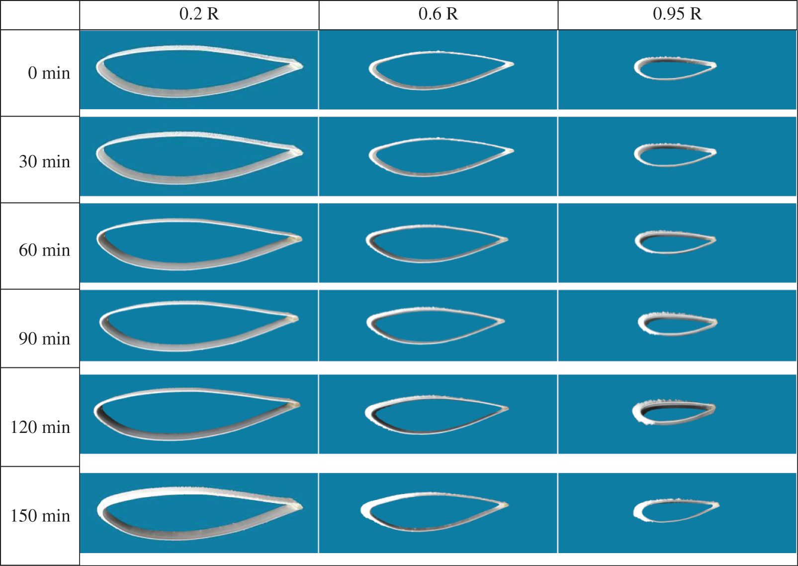
Figure 6: Test result photographs
The ice thickness increases with time, and the amount of accumulated ice notably alternates alongside the blade span. The highest and lowest ice thicknesses occur at 0.95 and 0.2 R, respectively. In the experiment, the blade ice type corresponds to the glaze ice, which initially forms at the 0.95 R monitoring position and then spreads towards the 0.6 R position. The most apparent ice angle is observable at 0.95 R, and the “feather-shaped” ice grows as the experiment progresses. Assessments at the positions 0.6 and 0.95 R for t = 120 min are chosen as the statement samples, as illustrated in Fig. 7.
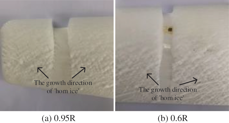
Figure 7: Glaze ice attached to blades
4.2 Effect of Icing on the Airfoil Chord Length
The icing of wind turbine blades changes the airfoil shape. Because of continuous adhesion, the ice formation steadily changes the geometric airfoil parameters and reduces the aerodynamic characteristics of the blade. Analysis of the test results at the monitoring positions 0.95, 0.6, and 0.2 R shows that the most considerable ice thickness occurs at the leading edge (point 1). Ice formation at this point significantly changes the chord length. The present section analyzes the influence of icing on the airfoil chord length based on a rectangular coordinate system. The airfoil leading edge is considered as the coordinate origin, the chord length direction is assigned as the x-axis. The normal direction to the chord length indicates the y-axis, as depicted in Fig. 8.
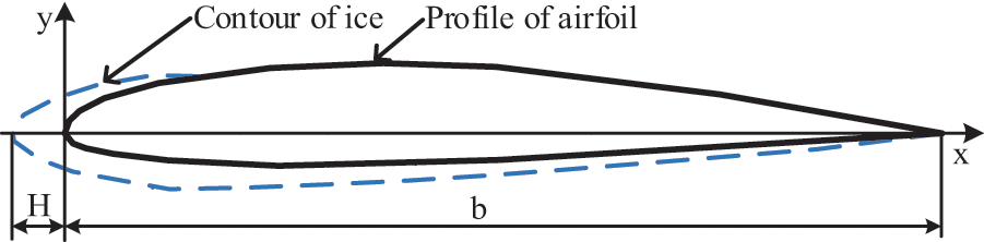
Figure 8: Effect of icing on the chord length
Fig. 9 illustrates the temporal variation of the ice thickness at the airfoil leading edge for three monitoring positions. The highest and lowest ice layer contents exist for the 0.95 and 0.2 R, respectively. Furthermore, the ice layer at the leading edge of the 0.95 R position has the fastest growth rate, which may cause a significant power loss. In contrast, the results obtained for the ice layer growth at 0.2 R are very uncertain.
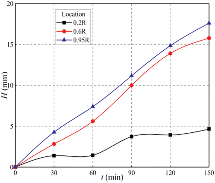
Figure 9: Ice thickness at the airfoil leading edge
Two reasons are responsible for the phenomenon mentioned above:
(1) The wind turbine has a high speed at the initial stage of the icing test. The cooled water droplets are therefore subjected to a large centrifugal force with a strong radial flow potential. As a result, the cooled water droplets migrate radially from the blade root and accumulate at the blade tip.
(2) The blade tip linear speed is higher than the blade root speed. Therefore, the collision efficiency of cooled water droplets is the highest at the blade tip. At the same time, the blade tip profile can seize a more significant amount of cooled water droplets.
4.3 The Effect of Icing on the Airfoil Camber
4.3.1 Changes in the Airfoil Camber and Maximum Camber Position
This section investigates the impact of the icing process on the airfoil camber and the variation of the maximum camber position based on a mathematical model established for the airfoil icing. After defining a suitable coordinate system, the curve equation for the airfoil camber is obtained by numerical fitting, and the influence of icing on the airfoil camber is analyzed quantitatively. The coordinate system is defined as described above and is illustrated in Fig. 10.
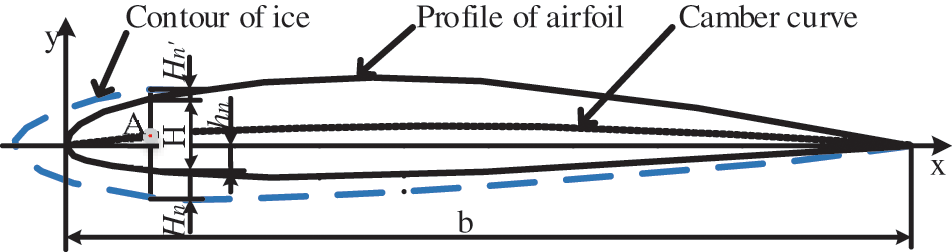
Figure 10: Effect of icing on the airfoil camber
Based on the measured data in each test, the curvature model is established as expressed by Eq. (1).
where, i is the different monitoring positions (i = 0.2, 0.6, 0.95);
According to the parameters presented in Tables 2 and 3 (calculated using Eq. (1)), each measurement point is calculated separately to obtain the coordinates of the airfoil camber after the icing process. The camber coordinate data of the measurement points is then imported into the ORIGIN software to fit the airfoil’s camber curve equation to fit the airfoil equation under different freezing conditions. The fourth-order polynomial curve of the camber is obtained after multiple fittings, as expressed by Eq. (2).
where,
The camber value at any position along the chord length direction can be calculated from Eq. (2). The R2 test (the ratio of the regression sum of squares to the total sum of square deviations) is performed to evaluate the resulting equation’s fitting quality. Achievement of R2 > 94.8% indicates high regression quality of the fitting equation. Table 6 presents the curve equation coefficients for different icing times. The curve equation diagrams for the monitoring positions 0.95, 0.6, and 0.2 R are illustrated in Fig. 11.
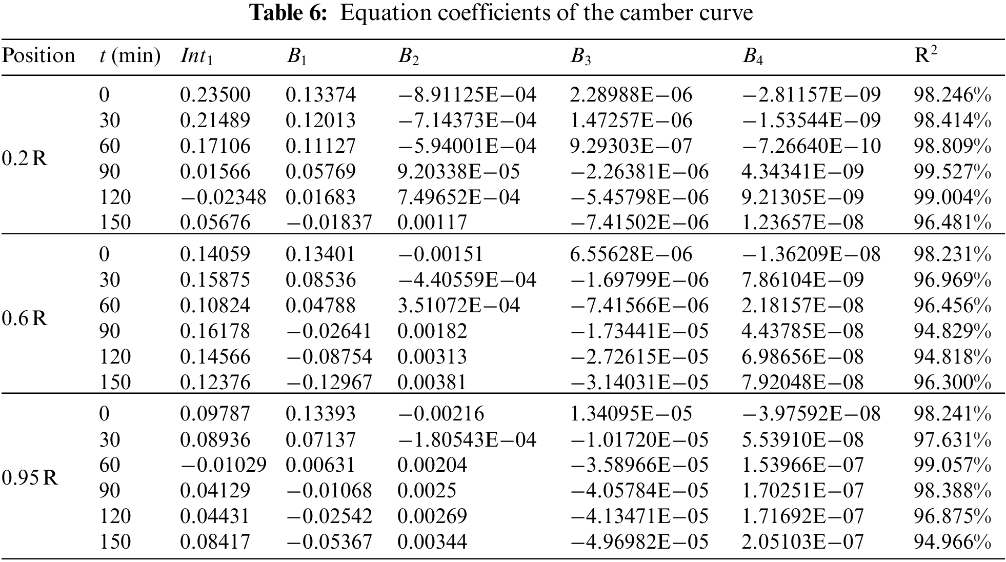
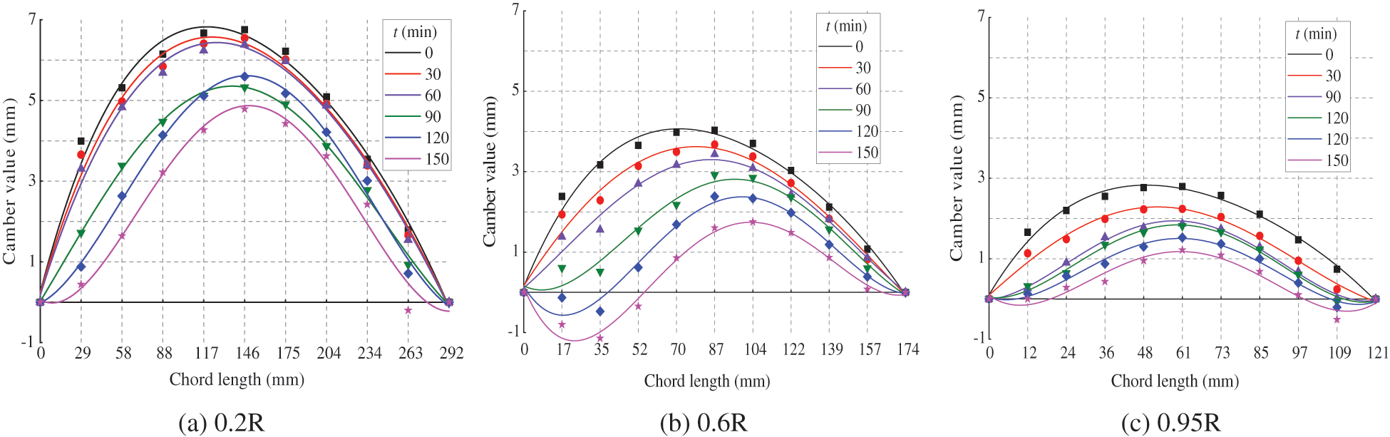
Figure 11: Curve fitting result of icing airfoil
Fig. 11 shows that the maximum curvature at the monitoring positions 0.95, 0.6 and 0.2 R gradually decreases by icing progress. Additionally, the maximum camber position tends to move towards the trailing edge. It can be clearly observed from Figs. 11b and 11c that the camber curve at the proximity of either the leading edge or trailing edge of the blade gradually displaces below the chord line as the icing evolves. The reason is that the icing mainly happens on the lower airfoil surface, which steadily grows downward. MATLAB 2014 software is utilized to obtain the coordinates corresponding to the maximum value of the right equation in order to study the curvature deviation during the test.
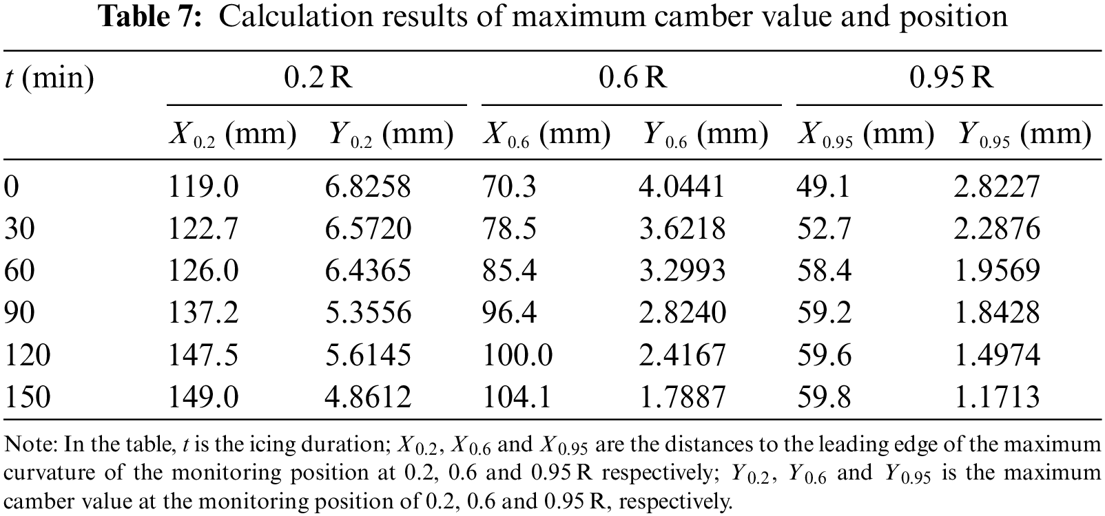
In the iterative calculation procedure, the design step size is 0.1. The calculation intervals involve the chord length values of 0.95, 0.6, and 0.2 R monitoring positions. The calculation results are listed in Table 7. Based on the results for three monitoring positions, the maximum camber position is moved towards the trailing edge as the icing evolves. At the end of the test and compared to the original state, the maximum curvature at the monitoring positions 0.2, 0.6, and 0.95 R reduces to 72.22%, 44.23%, and 41.50% based on the original value, respectively. Additionally, in comparison with the original airfoil, the maximum camber position shifts backward by 10.27%, 19.43%, and 8.84%, respectively.
4.3.2 Changes in the Position of Maximum Camber and Relative Camber
According to the data presented in Table 7, the position of the maximum camber and variation trend of relative camber are extracted, and the results are shown in Fig. 12. The x-axis in Fig. 12a indicates the ice coating duration of the test, y-axes correspond to the ice monitoring position, and the z-axis demonstrates the ratio of the chord length where the maximum camber position is located. By icing progress, this figure indicates that the maximum camber position of the airfoil at three monitoring positions steadily moves towards the trailing edge, and the offset of the maximum camber position at 0.6 R is the most obvious one.
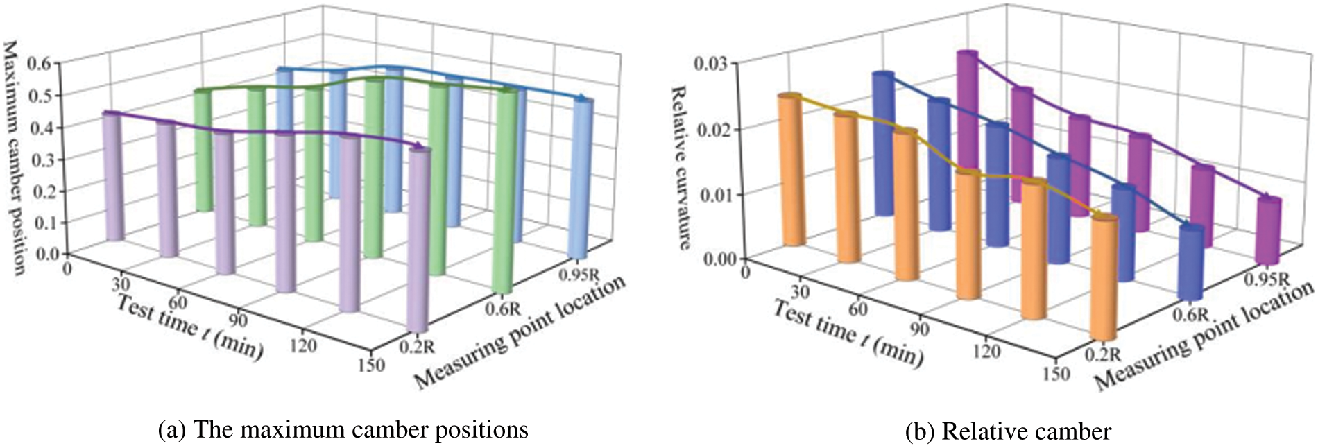
Figure 12: Variation of the maximum camber position and relative camber on the airfoil
The x, y, and z-axes in Fig. 12b indicate the length of the icing test, the ice monitoring positions, and the relative camber, respectively. A decreasing trend can be observed for the relative camber of the airfoil at three monitoring positions. The most obvious downward trend occurs at the 0.95 R position, which can be used to estimate the offset of different ice times, relative curvatures and maximum curvature positions.
4.4 The Impact of Icing on the Airfoil Thickness
4.4.1 Changes in the Airfoil Thickness and Maximum Thickness Position
This section examines the influence of icing on the airfoil thickness as well as the maximum airfoil thickness position based on the mathematical model constructed for airfoil icing. Based on a suitable coordinate system and numerical fitting, a mathematical model of the airfoil thickness is established in order to analyze the icing effect on airfoil thickness quantitatively. The coordinate system is defined as described previously, and it has been illustrated in Fig. 10.
In this section, the thickness coordinate model is established by analyzing the measurement point data of each test, as presented in Eq. (3).
where,
According to the parameters given in Tables 2 and 3, the thickness at each measurement point is calculated using Eq. (3). It is then converted to the thickness coordinate of the measurement point, and this coordinate is imported into the ORIGIN software. The mathematical model of airfoil thickness is fitted for various icing thicknesses. The fifth-order polynomial curve of the airfoil thickness is obtained after multiple fittings, as expressed in Eq. (4). It can be used to calculate the thickness at any position along the chord length direction. Evaluation of the fitted equation by the R2 test (R2 > 94.6%) shows that the established mathematical model has a high regression quality. Table 8 presents the coefficients of the thickness curve equation for various icing conditions. Furthermore, Fig. 13 illustrates the thickness curve equation plots for the monitoring positions 0.95, 0.6, and 0.2 R.
where,
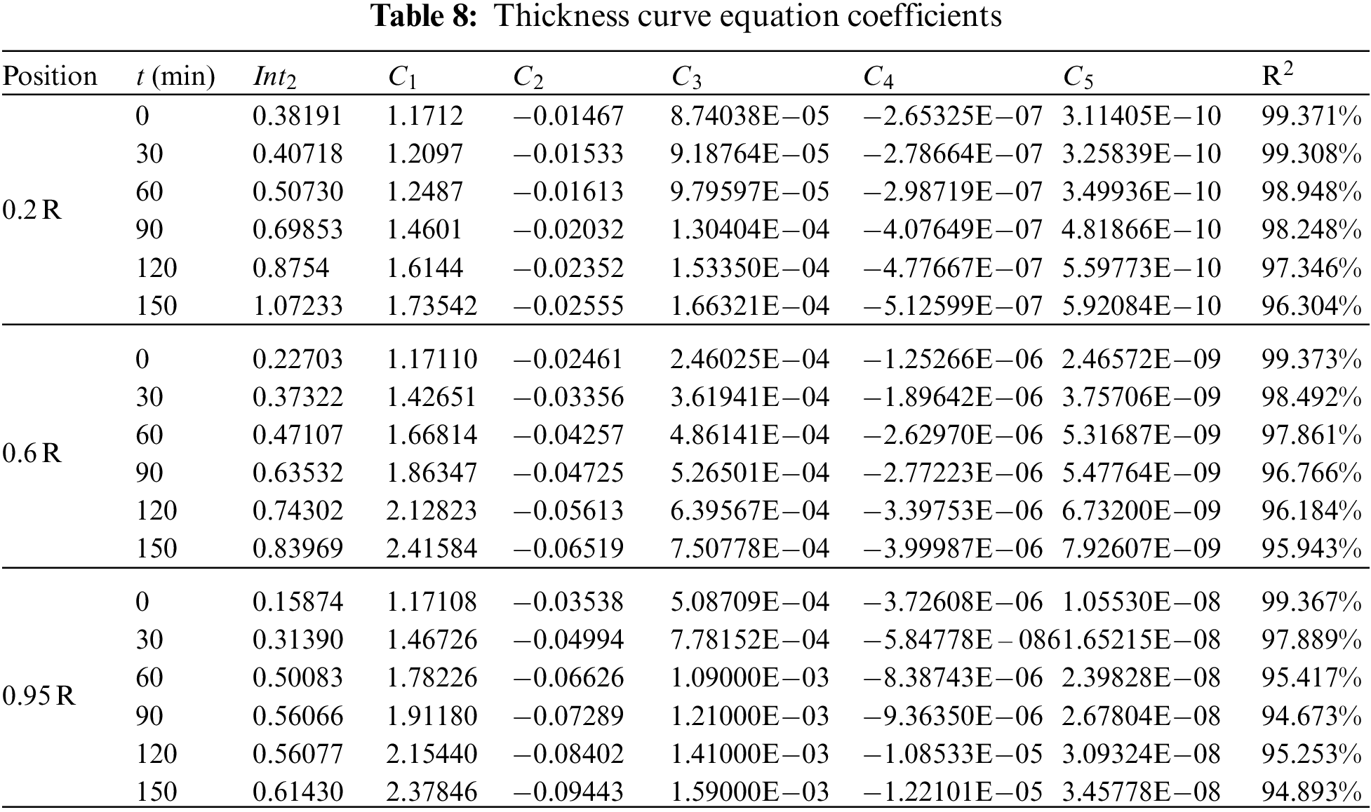
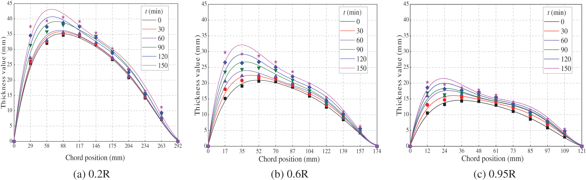
Figure 13: Thickness distribution and curve fitting of icing airfoil
It can be observed from Fig. 13 that the maximum thickness of the monitoring positions gradually increases in time. As the test continues, the maximum thickness position moves towards the leading edge. The reason is the increase in distance between the upper and lower surfaces of the airfoil by growing the ice layer which increases the airfoil thickness. In order to quantitatively analyze the maximum thickness deviation with respect to the trailing edge during the test, MATLAB software is used to obtain the fitting equation coefficients.
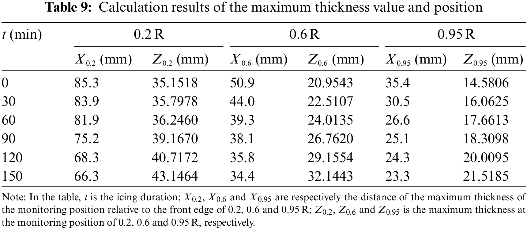
The design step size in the iterative procedure is again considered to be 0.1. The maximum value of the operation interval corresponds to the chord length at the positions 0.95, 0.6, and 0.2 R. The calculation results are listed in Table 9. Based on the results, the maximum thickness of three monitoring positions is increased by icing progress. Furthermore, the maximum thickness position moves towards the leading edge. In comparison with the original state, the maximum thickness for the monitoring positions 0.2, 0.6 and 0.95 R increases by 22.74%, 53.40%, and 47.58%, respectively. Furthermore, the maximum thickness position is shifted towards the leading edge by 6.51%, 9.48%, and 10.00%, respectively.
4.4.2 Changes in the Maximum Thickness Position and Relative Thickness
According to the data presented in Table 9, variation in the maximum thickness position and the relative thickness can be analyzed, as illustrated in Fig. 14. The x-axis in Fig. 14a demonstrates the duration of the icing test, the y-axis is for the ice monitoring position, and the z-axis indicates the ratio of chord length at the position of maximum thickness. According to the results, the maximum thickness position of the airfoil at three monitoring positions moves towards the leading edge as the icing evolves. Additionally, the most obvious offset of the maximum thickness position happens at 0.95 R.
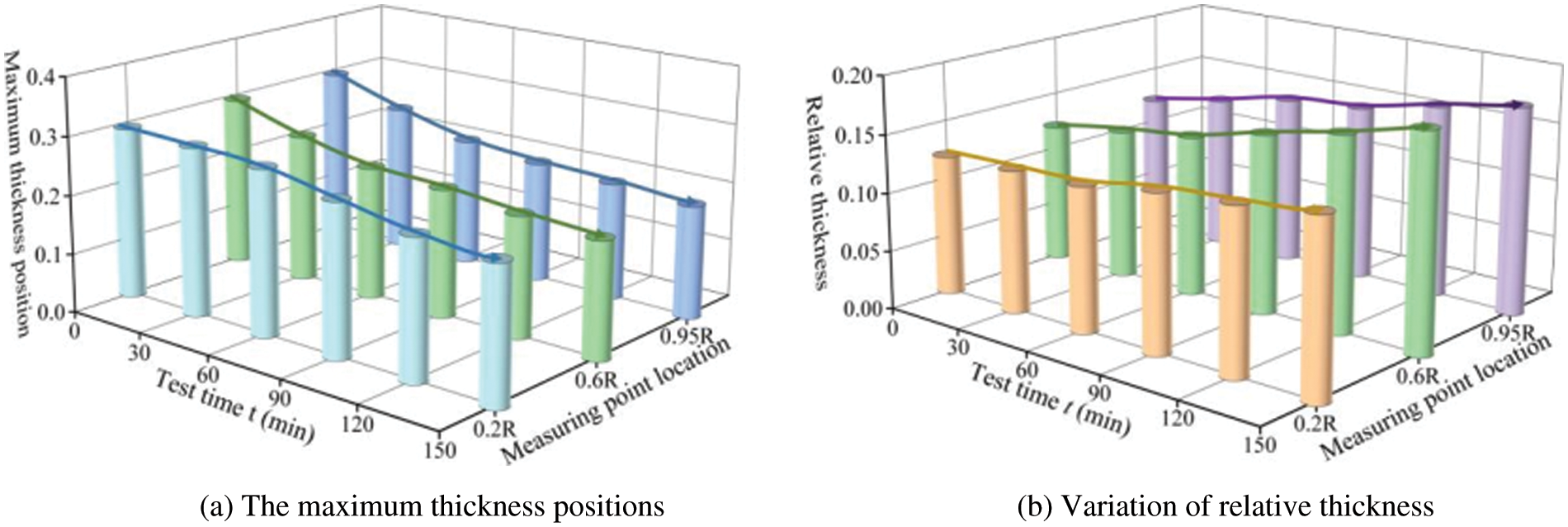
Figure 14: Variation of the maximum thickness position and relative thickness on the airfoil
The x-axis in Fig. 14b represents the length of the icing test, the y-axis is for the ice monitoring position, and the z-axis denotes the relative thickness value. An ascending trend is observed for the relative thickness of the airfoil at three monitoring positions as the icing develops. The most evident variation trend exists at the 0.6 R position. Fig. 14 can estimate the variation of ice duration, relative thickness, and maximum thickness.
The present study analyzed the icing distribution along with the wind turbine blades in the natural low-temperature condition. A novel measurement method was proposed to determine the ice accumulation extent around the airfoil accurately. The mathematical model of the chord length, camber, and thickness with respect to the ice content was subsequently established. This model was designed to quantitatively examine the changes in blade airfoil geometric parameters during the dynamic icing process. This provides a theoretical foundation and technical prerequisite for further research on the adverse impact of icing on the overall aerodynamic performance of the airfoil.
The concluding remarks of the present study are as follows: 1. By icing progress, the chord length of the airfoil increases, and the most significant variation occurs at the 0.95 R position; 2. during the icing process, the airfoil camber decreases steadily, and the maximum camber position moves towards the trailing edge; 3. The maximum thickness significantly increases by icing progress, and the most obvious variation exists at the middle of the blade. The maximum thickness position moves towards the leading edge, which clearly explains why airfoil aerodynamics deteriorates by icing growth. Furthermore, the blade design was based on the blade element momentum theory, whether the wind turbine is a horizontal-axis or a vertical-axis type. The proposed research method in the present study, which relies on a variety of geometric airfoil parameters induced by the icing process, is also applicable to the related research problems in the vertical-axis wind turbine blades.
Variation of the blade surface roughness decreases its aerodynamic characteristics. This opens a future research plan in which the impact of ice accumulation on the variation of the blade surface roughness and its aerodynamic consequences can be examined. Under icing conditions, a larger turbulent wake can also be generated downstream of the blade surface, which deserves more in-depth analysis in the future.
Author Contributions: Conceptualization, H. Z. and X. L.; Data curation, Y. J., X. L. and H. Z.; Formal analysis, X. L.; Funding acquisition, B. C.; Methodology, H. Z. and X. L.; Project administration, H. Z. and X. L.; Resources, X. L. and B. C.; Software, Y. J.; Supervision, Y. J. and X. L.; Validation, Y. J. and X. L.; Visualization, H. Z.; Writing–original draft, Y. J.; Writing–review & editing, H. Z., B. C. and X. L. All authors have read and agreed to the published version of the manuscript.
Data Availability: All data included in this study are available upon request by contact with the corresponding author.
Funding Statement: This work was supported by a grant of National Natural Science Foundation of China, Grant No. 51665052.
Conflicts of Interest: The authors declare that they have no conflicts of interest to report regarding the present study.
REFERENCES
1. Wang, Z., Zhu, C. (2018). Numerical simulation for in-cloud icing of three-dimensional wind turbine blades. Simulation: Transac-tions of the Society for Modeling and Simulation International, 94(1), 31–41. DOI 10.1177/0037549717712039. [Google Scholar] [CrossRef]
2. Papi, F., Cappugi, L., Salvadori, S., Carnevale, M., Bianchini, A. (2020). Uncertainty quantification of the effects of blade damage on the actual energy production of modern wind turbines. Energies, 13(15), 3785. DOI 10.3390/en13153785. [Google Scholar] [CrossRef]
3. Yirtici, O., Tuncer, I. H. (2021). Aerodynamic shape optimization of wind turbine blades for minimizing power production losses due to icing. Cold Regions Science & Technology, 85, 103250. DOI 10.1016/j.coldregions.2021.103250. [Google Scholar] [CrossRef]
4. Guo, W. F., He, S., Li, Y., Feng, F., Tagawa, K. (2021). Wind tunnel tests of the rime icing characteristics of a straight-bladed vertical axis wind turbine. Renewable Energy, 179, 116–132. DOI 10.1016/j.renene.2021.07.033. [Google Scholar] [CrossRef]
5. Martini, F., Contreras, M., Leidy, T., Ilinca, A. (2021). Review of wind turbine icing modelling approaches. Energies, 14(16), 5207. DOI 10.3390/en14165207. [Google Scholar] [CrossRef]
6. Jin, J. Y., Virk, M. S., Hu, Q., Jiang, X. L. (2020). Study of ice accretion on horizontal axis wind turbine blade using 2D and 3D numerical approach. IEEE Access, 8, 166236–166245. DOI 10.1109/Access.6287639. [Google Scholar] [CrossRef]
7. Han, W., Kim, J., Kim, B. (2018). Study on correlation between wind turbine performance and ice accretion along a blade tip airfoil using CFD. Journal of Renewable & Sustainable Energy, 10(2), 023306. DOI 10.1063/1.5012802. [Google Scholar] [CrossRef]
8. Liu, Y., Hu, H. (2018). An experimental investigation on the unsteady heat transfer process over an ice accreting airfoil surface. International Journal of Heat and Mass Transfer, 122, 707–718. DOI 10.1016/j.ijheatmasstransfer.2018.02.023. [Google Scholar] [CrossRef]
9. Liu, Y., Li, L., Li, H., Hu, H. (2018). An experimental study of surface wettability effects on dynamic ice accretion process over an UAS propeller model. Aerospace Science and Technology, 73, 164–172. DOI 10.1016/j.ast.2017.12.003. [Google Scholar] [CrossRef]
10. Gao, L. Y., Liu, Y., Zhou, W. W., Hu, H. (2019). An experimental study on the aerodynamic performance degradation of a wind turbine blade model induced by ice accretion process. Renewable Energy: An International Journal, 133, 663–675. DOI 10.1016/j.renene.2018.10.032. [Google Scholar] [CrossRef]
11. Wang, Q., Xiao, J. P., Shi, Y., Wang, Q., Yang, J. J. et al. (2020). Study on the wind turbine icing computational model based on the dynamic analysis of liquid film. Journal of Engineering Thermophysics, 41(7), 1666–1672. [Google Scholar]
12. Gao, L. Y., Hong, J. R. (2021). Wind turbine performance in natural icing environments: A field characterization. Cold Regions Science & Technology, 181, 103193. DOI 10.1016/j.coldregions.2020.103193. [Google Scholar] [CrossRef]
13. Jin, J. Y., Virk, M. S. (2020). Experimental study of ice accretion on S826 & S832 wind turbine blade profiles. Cold Regions Science & Technology, 169, 102913. DOI 10.1016/j.coldregions.2019.102913. [Google Scholar] [CrossRef]
14. Bragg, M. B., Gregorek, G. M., Lee, J. D. (1986). Airfoil aerodynamics in icing conditions. Journal of Aircraft, 23(1), 76–81. DOI 10.2514/3.45269. [Google Scholar] [CrossRef]
15. Li, D. S., Dong, L., Liu, Y., Li, R. N., Li, Y. R. et al. (2015). The influence of wind and sand environment on the aerodynamic performance of NACA-0012 airfoil. Journal of Lanzhou University of Technology, 41(6), 54–59. [Google Scholar]
16. Li, K. L., Lu, X. X., Chen, Z. G., Yang, B., Tan, T. et al. (2017). Numerical study on aerodynamic performance of wind turbine blade airfoil based on fluent. Energy and Environment, 5, 40–42. [Google Scholar]
17. Sundaresan, A., Arunvinthan, S., Pasha, A. A., Pillai, S. N. (2021). Effect of ice accretion on the aerodynamic characteristics of wind turbine blades. Wind & Structures, 32(3), 205–217. [Google Scholar]
18. Zhang, X., Zhang, X. Y., Wang, G. G., Li, W. (2020). Effects of blunt trailing-edge optimization on aerodynamic characteristics of NREL phase VI wind turbine blade under rime ice conditions. Journal of Vibroengineering, 22(5), 1196–1209. DOI 10.21595/jve. [Google Scholar] [CrossRef]
19. Lamraoui, F., Fortin, G., Benoit, R., Perron, J., Masson, C. (2014). Atmospheric icing impact on wind turbine production. Cold Regions Science and Technology, 100, 36–49. DOI 10.1016/j.coldregions.2013.12.008. [Google Scholar] [CrossRef]
20. Zhang, X., Wang, G. G., Zhang, M. J., Li, W. (2017). Effect of relative camber on the aerodynamic performance improvement of asymmetrical blunt trailing-edge modification. Journal of Engineering Thermophysics, 26(4), 514–531. DOI 10.1134/S1810232817040075. [Google Scholar] [CrossRef]
21. Liu, Q., Miao, W., Li, C., Hao, W., Deng, Y. (2019). Effects of trailing-edge movable flap on aerodynamic performance and noise characteristics of VAWT. Energy, 189, 116271. DOI 10.1016/j.energy.2019.116271. [Google Scholar] [CrossRef]
22. Liu, H. P., Wang, Y., Yan, R. J., Xu, P., Wang, Q. (2020). Influence of the modification of asymmetric trailing-edge thickness on the aerodynamic performance of a wind turbine airfoil. Renewable Energy, 147, 1623–1631. DOI 10.1016/j.renene.2019.09.073. [Google Scholar] [CrossRef]
23. Zhang, Y., Ye, J. J., Huang, X. H., Ji, R. Y., Li, W. J. (2020). Aerodynamic performances of the wind turbine airfoils in the condition of low wind speed. International Journal of Fluid Dynamics, 8(1), 1–8. DOI 10.12677/IJFD.2020.81001. [Google Scholar] [CrossRef]
24. Fakorede, O., Feger, Z., Ibrahim, H., Ilinca, A., Perron, J. et al. (2016). Ice protection systems for wind turbines in cold climate: Characteristics, comparisons and analysis. Renewable & Sustainable Energy Reviews, 65, 662–675. DOI 10.1016/j.rser.2016.06.080. [Google Scholar] [CrossRef]
25. Liao, W., Wei, M. M., Huang, Y. Y. (2008). Study on raindrop diameter by filter paper stain method. Journal of Wuhan University of Technology (Traffic Science and Engineering), 32(6), 1165–1168. [Google Scholar]
26. Zhang, Z. J., Zhang, Y., Jiang, X. L., Hu, J. L., Hu, Q. (2018). Icing degree characterization of insulators based on the equivalent collision coefficient of standard rotating conductors. Energies, 11(12), 3326. DOI 10.3390/en11123326. [Google Scholar] [CrossRef]
Cite This Article
 Copyright © 2022 The Author(s). Published by Tech Science Press.
This work is licensed under a Creative Commons Attribution 4.0 International License , which permits unrestricted use, distribution, and reproduction in any medium, provided the original work is properly cited.
 Downloads
 Citation Tools