Short-Term Wind Power Prediction Based on ICEEMDAN-SE-LSTM Neural Network Model with Classifying Seasonal

Nomenclature

1  Introduction

With the emphasis and efforts on environmental protection and the transformation of traditional energy structures, the scale of wind power grid integration is rapidly expanding. However, the inherent volatility and randomness of wind power bring severe challenges to wind power grid integration. Therefore, accurate prediction of wind power efficiency is of great significance to properly arrange system backup, thus ensuring stable operation and improving the economic benefits of power grids [1–4].

Nowadays, worldwide scholars and engineers have carried out in-depth research on wind power prediction and achieved remarkable results. With the development of wind power industry, the configuration of wind farms has gradually changed from distributed distribution to regional distribution [5–7]. The references available suggest that meteorological observation points adjacent to renewable energy stations can also provide valuable information [8–10]. With the rise of artificial intelligence, methods such as neural network and deep learning have demonstrated satisfactory capabilities in mining data features and processing data [11,12].

In reference [13], an improved aggregated probabilistic wind power forecasting framework based on spatiotemporal correlation is developed to forecast wind power intervals, but high dimensional matrices are involved in the spatiotemporal modeling, which results in additional computational burden. Reference [14] proposed a short-term interval prediction method based on variational mode decomposition and phase correlation vector machine, whose prediction result strictly depends on the selection of kernel function. In reference [15], a bootstrap resampling method is used to construct pseudo-samples to obtain the predicted power error interval, which needs to process a large amount of data that might lead to a long computation time. Reference [16] estimated the error distribution function of sensitive meteorological factors and proposed a Monte-Carlo random sampling method to obtain the interval prediction results, which need to be supported by meteorological data. Reference [17] carried out fuzzy informatization of noise components and established a wind speed interval prediction model based on an extreme learning machine, but its time-series memory ability is not strong. With the extensive application of deep learning, its advantages in temporal memory and feature mining of data have been revealed.

Since there are many factors affecting wind power output, it is difficult for a single model to cover all the factors, such that its prediction results tend to be considered uncertain to some extent. Therefore, some scholars have combined the predictions of multiple models, which can be categorized into weighted combination prediction and fusion combination prediction [18]. Based on the idea of ensemble learning, references [19,20] carried out weighted summation of prediction results from multiple same or different networks to obtain the final prediction results. However, due to overfitting, excessive integration time leads to a decrease in accuracy. Reference [21] combined convolutional neural network and radial basis neural network together, and adopted a double-layer Gaussian kernel as kernel function to improve the fitting ability of the network. However, this method needs to be supported by more (or at least the same size) sampled input data from different meteorological stations to obtain more accurate day-ahead forecasting. Therefore, it is necessary to develop a data preprocessing algorithm that can eliminate the negative impact of outliers and spurious data on prediction performance. Based on the aforementioned discussion, a short-term wind power forecasting method based on improved complete ensemble empirical mode decomposition with adaptive noise (ICEEMDAN) and (long short-term memory) LSTM is proposed in this work to address the existing shortcomings of individual methods. First, the random forest algorithm is employed to screen the most important meteorological factor. Secondly, ICEEMDAN is utilized to decompose the original wind power series into multiple modal components, and sample entropy (SE) is used for reconstruction. Finally, LSTM is adopted to carry out the wind power prediction.

The remainder of this work is organized as follows: Section 2 introduces the data preprocessing of wind power data. Section 3 describes the mechanism of wind farm data decomposition and mode function reconstruction. Section 4 illustrates the wind power prediction model under seasonal classification. Section 5 presents a detailed analysis of the simulation results. Finally, Section 6 presents several critical conclusions and perspectives.

2  Wind Power Data Preprocessing of Outliers

Wind power measurement data can be regarded as a set of time series with random fluctuations, while the original time series data may have a large number of outliers or defects caused by extreme weather, erroneous records, or sensor failures. These data will directly affect the training stage of the prediction model, thereby affecting the prediction performance of the model. The preprocessing of defect data is the fundamental step for wind power prediction. In addition, the original historical information of wind farms includes wind speed, wind direction, temperature, air pressure, atmosphere humidity and other related meteorological information and historical power data. However, excessive feature inputs do not necessarily mean higher prediction accuracy, on the contrary, they may negatively affect the precision of the prediction model. Therefore, it is necessary to screen the historical meteorological features based on the sufficient and proper utilization of historical information to avoid redundant input data and reduce the computational complexity of the prediction model. The uncertainty of wind power mainly comes from three aspects: meteorological factors, electric energy production, and electric energy transmission. The uncertainty of the prediction model should be considered in the wind power prediction as well.

Wind energy resources are very sensitive to weather changes. Meteorological information such as wind speed, wind direction, pressure, and temperature at different heights may have varying degrees of impact on wind power output. The meteorological factor itself has uncertainty, which affects the fluctuation of wind power. Numerical weather prediction (NWP) data is future meteorological data calculated based on atmospheric motion, which inevitably brings errors that are difficult to eliminate. In view of this, considering the fusion of multi-source and multi-type NWP data is an effective method to reduce the uncertainty of meteorological factors. The outputs of wind turbines are not only related to meteorological conditions, but also to their own running state and operating conditions. For example, under the same wind conditions, the output of wind turbines will vary depending on the state of the turbine. In addition, human factors in wind farms also affect the output level, meanwhile, personnel scheduling and decision-making in wind farm operations will also bring inestimable power uncertainty. For wind farm output prediction, it is crucial to build a model to estimate future output power value, so the influence of the model forecasting ability on the prediction results cannot be ignored. If the model assumptions used in the prediction are not reasonable, or the selection of a function relationship that maps future power is not appropriate, some uncertainty tends to be added to the prediction results. Whether using simple linear models to solve nonlinear problems or using complex nonlinear models to solve simple linear problems, it will reduce the precision of wind power prediction and bring great uncertainty to the prediction results.

The data used in this work is collected from the field test data of a wind farm in Hami, Xinjiang. The collected historical wind power data package includes wind speed, wind direction, temperature, atmosphere pressure, humidity, wind power, and six related variables. The height of data measurement includes 10, 30, 50 m, and hub height, and the time resolution is 15 min. A total of 35040 data samples, including missing values, were collected from 0:00 on January 01, 2019, to 24:00 on December 31, 2019. The rated capacity of the wind farm station is 201 MW. The annual wind power curve is shown in Fig. 1. As can be seen from Fig. 1, wind power has strong intermittent fluctuation characteristics, which will bring great difficulties in direct prediction.

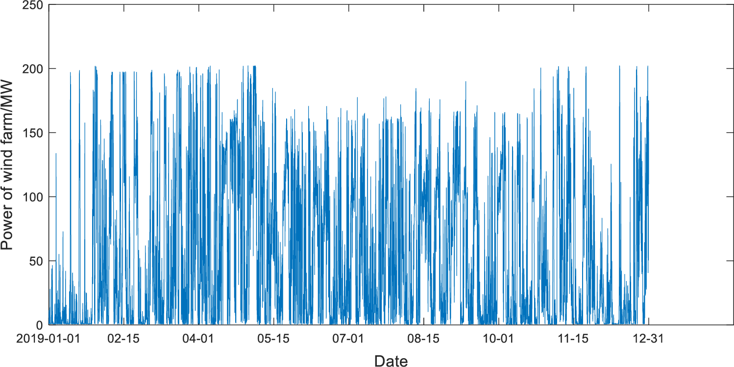
Figure 1: Scatter diagram of annual wind power

2.1 Outliers Data Processing

The quality of the original wind power data directly influences the prediction accuracy. A large number of wind farms are prone to abnormal data due to equipment and communication problems. If the abnormal data is not properly processed, it will bring great error to the prediction result. Therefore, it is necessary to carry out outlier tests, missing value filling, and data transformation of measured data before prediction. The wind power prediction data should not exceed the limit value, that is, the power value should not be less than zero. If it is less than zero, the wind speed may stop the unit because the wind speed is lower than the cut-in value or higher than the cut-out wind speed, resulting in power backdraft. In the experimental data used in this study, a small amount of data is lower than zero, even if the value is very small, it should still be discarded in the prediction.

Due to random failures of wind turbines, scheduled maintenance, communication signal interruption, and other reasons, most of the historical data recorded by wind farms are partially missing, resulting in low-quality original data, which brings great difficulties to accurate prediction. Therefore, it is necessary to process the missing value before prediction. The types of data loss can be divided into individual deletion, small deletion, and large deletion. The missing value can be filled according to the average power before and after the missing position. A small amount of missing data can be completed by interpolation method, and the completed data values are determined by

Xi+i0=Xi+Xi+i1−Xi1i1(1)

where Xi+i0 is power value of the (i+i0)th sampling point; Xi, Xi+i1 and Xi1 are the values of the ith, (i+i1)th, i1th sampling point.

A large number of data blocks may be lost due to scheduled maintenance or equipment failure. To supplement a large amount of missing data, the data values of nearby wind farms in the same time period can be referred to. If the data values of the nearby wind farms in the same period are very different, the missing data blocks for that time period will be deleted.

The meteorological conditions of nearby wind farms within the same time period have relatively small differences, and the errors basically meet the requirements. Direct deletion will result in the loss of training samples and a decrease in prediction accuracy. In contrast, using the data of nearby wind farms in the same time period can ensure the integrity of model training data and obtain more accurate prediction results.

To improve the convergence speed during training after the processing of abnormal data, the historical data of wind farm is normalized according to the following formula:

X∗=(X−Xmin)/(Xmax−Xmin)(2)

X=X∗⋅(Xmax−Xmin)+Xmin(3)

where Xmin is the minimum power value; Xmax is the maximum power value; X∗ is the power value after normalization; X is the power value inverse after normalization.

2.2 Feature Extraction Based on Random Forest Algorithm

Rough set, mutual information, and Pearson coefficient are common methods for feature selection of wind farm historical data. Most of these methods are extracted by analyzing the information entropy and correlation coefficient between meteorological characteristics and wind power. The quality of input data has a great influence on the result of feature extraction [22].

Random forest (RF) is a bagged algorithm based on a decision tree classifier. In feature engineering, important features can be extracted from random forests according to the impact of input features on prediction or classification results. Compared with the correlation coefficient and mutual information methods, random forest is less affected by noise data. The data in the random forest that does not participate in the construction of the training set of the decision tree is called the out-of-pocket data of the tree. If the number of RF decision trees is n, then the model training process can be described as follows: First, the out-of-pocket error rate emil of each decision tree is calculated according to the out-of-pocket data which can be expressed by Eq. (4). Then, keeping the characteristics of sample unchanged, random change the jth variable vj outside bag, and finally calculate the new out-of-pocket error rate emil′, so that the importance value M(vj) of characteristic variables of vj is calculated by Eq. (5).

emil=ierriall(4)

M(vj)=1N∑i=1N(emil′−emil)(5)

where ierr is the amount of prediction errors; iall is total number of samples; N represents total meteorological features. The accuracy decreases with the decrease of M(vj), and the more the accuracy decreases, the more important the meteorological feature is.

The experimental data used in this study is the measured data collected from a wind farm in Xinjiang. After removing abnormal data, the number of total wind power data samples is 34520, and the data resolution is 15 min. Take the data of the first month as an example to analyze the importance of meteorological characteristics to wind power output. Data set partitioning has a certain impact on RF results. After many experiments of partitioning different data sets, it is concluded that the model works best when 70% data of the data set is used for training and 30% is used for testing. The number of RF decision trees is 700 and the number of node candidate features is 4. The descending order of the importance results of each feature is shown in Table 1.

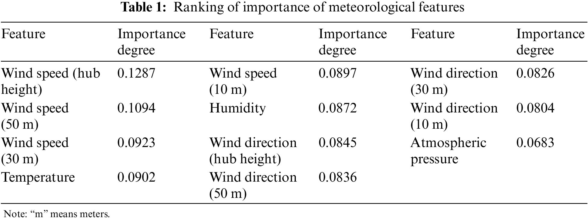
As can be seen from Table 1, wind speed at the hub height has the greatest impact on wind power output and the highest correlation, while atmospheric pressure has the smallest impact on wind power output and the lowest correlation. The final selected meteorological features are wind speed at hub height, wind speed at a height of 50 m, temperature and wind speed at a height of 10 m.

The prediction of wind power is influenced by multiple factors, and different factors have varying degrees of impact on the accuracy of the prediction model. According to their importance, wind speed has the greatest impact, followed by temperature, humidity, wind direction, and air pressure.

3  Wind Farm Data Decomposition and Mode Function Reconstruction

3.1 Decomposition of Wind Outputs Data Based on ICEEMDAN

ICEEMDAN, whose principle is different from empirical mode decomposition (EMD), utilizes the intrinsic mode functions (IMF) decomposed by the empirical mode decomposition method to solve the problem of residual noise and pseudo-modes. ICEEMDAN not only solves the problem of mode aliasing but also greatly reduces the residual noise in IMF. Besides, it has excellent decomposition and feature extraction ability for components of different scales contained in wind power time series. The basic steps for decomposing the power output of a wind farm using ICEEMDAN are as follows:

(1) x is assigned as the original wind power time series, and special noise Ek(wi) is added to x, as shown in the following equation:

xi=x+α1Ek(wi)(6)

where α1 is the iterative expected signal-to-noise ratio in the first decomposition; Ek(⋅) means the k-order mode function decomposed by EMD; wi represents the ith group white noise contributing to decomposition; xi is the wind power time series with the ith group special noise;

(2) Compute the residual error r1 of the first decomposition as following equations, and the mode function d1 is obtained by subtracting the residual from the original wind power rate time series x:

r1=1I+∑i=1IM(x+α1Ek(wi))(7)

d1=x−r1(8)

where M(⋅) denotes an operator that generates the local mean of a signal; I represents the number of white noise groups;

(3) Continue to add the white noise signal, calculate the second residual r2, and obtain the second order mode function d2 of the original power time series, as follows:

r2=1I+∑i=1IM(r1+α2E2(wi))(9)

d1=r1−r2(10)

(4) Similarly to step (3), calculate the kth residual error and mode function, as follows:

rk=1I+∑i=1IM(rk−1+αkEk(wi))(11)

dk=rk−1−rk(12)

(5) Repeat step (4) until the maximum number of iterations is reached or residuals can no longer be decomposed.

3.2 Wind Power Mode Function Reconstruction Based on Sample Entropy

If all the modal components (i.e., IMFs) obtained from mode decomposition are directly predicted separately, the calculation amount will be greatly increased and the correlation between the sub-components will be ignored. The classification and reprocessing of correlated components can not only shorten the computing time, but also highlight the characteristics of the same-type components. Therefore, the entropy law of information theory is used to deal with the sub-components.

Sample entropy is an improved method to measure the complexity of time series based on approximate entropy [23]. The lower the value of sample entropy, the higher the self-similarity and the lower the complexity of the time sequence. Compared with approximate entropy, sample entropy does not depend on data length and has better consistency. The formula of SE is given as follows:

Sampen(m,r,n)=−Ln[Bm+1(r)Bm(r)](13)

where L is the length of mode component; Bm+1(r) and Bm(r) are the probability of matching m and (m+1) points in the sequence under the tolerance r, respectively; in the actual scenario, m is the dimension, which is usually assigned as 2; r is the tolerance, usually calculated as 10%~25% of the standard deviation of the calculated data. In this study, r = 0.2SD.

Considering that there are too many subcomponents after decomposition, meanwhile, data processing and training are both time-consuming all the decomposed subcomponents are modeled and predicted directly, and SE is used to evaluate the complexity of each subcomponent. And then the components with similar SE are reconfigured into three components: trend, oscillation, and random components before the prediction.

4  Wind Power Prediction Model under Seasonal Classification

4.1 Seasonal Classification

Wind speed mutation is the main weather factor leading to power mutation [24]. The weather system is an unstable dynamic system, which means under different meteorological conditions, wind speed fluctuates differently, and the wind speed presents different change rules along with seasonal changes. Analysis of its rules is helpful in improving the accuracy of wind power prediction. This work defines five characteristic indicators, namely, mean value (μ), variance (σ2), variable coefficient (cv), asymmetry coefficient (λ1), and peak coefficient (λ2), to measure the temporal characteristics of NWP wind speed in different seasons.

μ=1n∑i=1nxi(14)

σ2=1n∑i=1n(xi−μ)2(15)

cv=σμ(16)

λ1=1n∑i=1n(xi−μ)3[σ2]3/2(17)

λ2=1n∑i=1n4[σ2]3/2(18)

The statistics of characteristic indicators of the studied wind farm in different seasons are shown in Table 2.

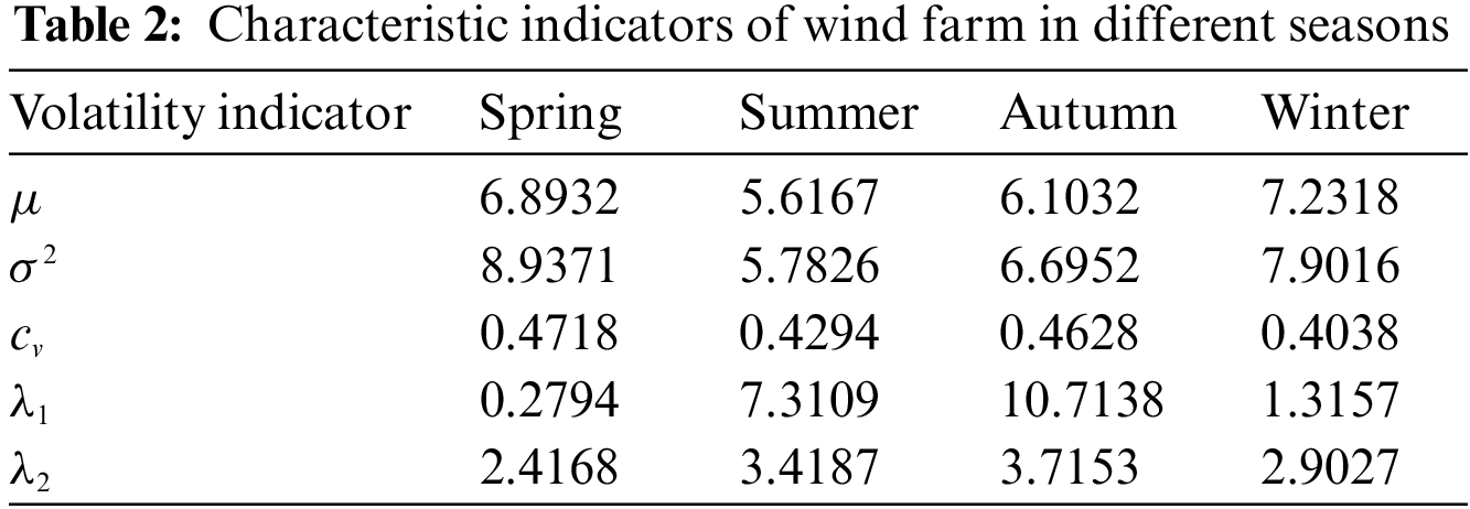
According to Table 2, the analysis is as follows: mean value (μ) and variance (σ2) are employed to measure the central tendency and the degree of dispersion of data; the mean value (μ) and variance (σ2) in summer are smaller than seasons, which indicates wind speed is smaller and most concentrated in summer; the mean value (μ) of winter is the largest, and the variance (σ2) is relatively larger than that in summer and autumn, which indicates that the winter wind speed value is larger and more discrete. The wind velocity value and dispersion degree in spring and autumn are between that value in summer and winter. Variable coefficient (cv) is used to measure the distribution of data form, i.e., the overall volatility of observed values. The variable coefficient (cv) in winter is the smallest, followed by summer, suggesting that these two seasons have relatively small changes based on average values and are generally relatively stable. However, the degree of variation in spring and autumn is significant, indicating significant fluctuations in wind speed.

The asymmetry coefficient (λ1) is used to measure the asymmetry of data. As far as coefficient λ1 is concerned, there are significant differences between the four seasons. The skewness degree in autumn is the largest, followed by summer, and the skewness degree in spring and winter is very small. Moreover, λ1 of four seasons are all positive, indicating that spring and summer present obvious right-side long-tail characteristics. There are more extreme values on the right side of the data mean, while the skewness degree in autumn and winter is basically the same as that of Gaussian distribution, i.e., the data is basically concentrated near the mean.

Peak coefficient (λ2) is used to measure the sharp degree of data. As far as coefficient λ2 is concerned, the wind speed tendency in spring is the steepest with the highest and sharpest peaks, while that in autumn is the smallest and smoothest. This indicates that the values of outlier data in spring are more extreme with the highest peak, whereas in autumn, it is in the middle of summer and winter. To sum up, the characteristic indices vary in different seasons, and wind speed fluctuations exhibit different characteristics.

4.2 Introduction to Prediction Model

In this work, two representative models are used to perform wind power prediction. The backpropagation (BP) network is usually used to deal with the input/output mapping relationship of multidimensional data, but traditional BP networks have slow convergence speeds and are prone to overfitting. To solve this, meta-heuristic algorithms offer an ideal tool to optimize the weights and thresholds of the BP network, thereby improving the prediction and approximation capabilities of BP neural network models. In this study, a genetic algorithm (GA) is selected to optimize the weight threshold between each layer of the BP network model. The structure of the GA-BP network is demonstrated in Fig. 2. In addition, the objective function of GA is the mean square prediction error of the training data, which can be calculated as follows:

f=∑i=1n(ui−vi)2(19)

where n is number of output nodes; ui is the expected output of the ith node of BP neural network; vi is the predicted output of the ith node of BP neural network.

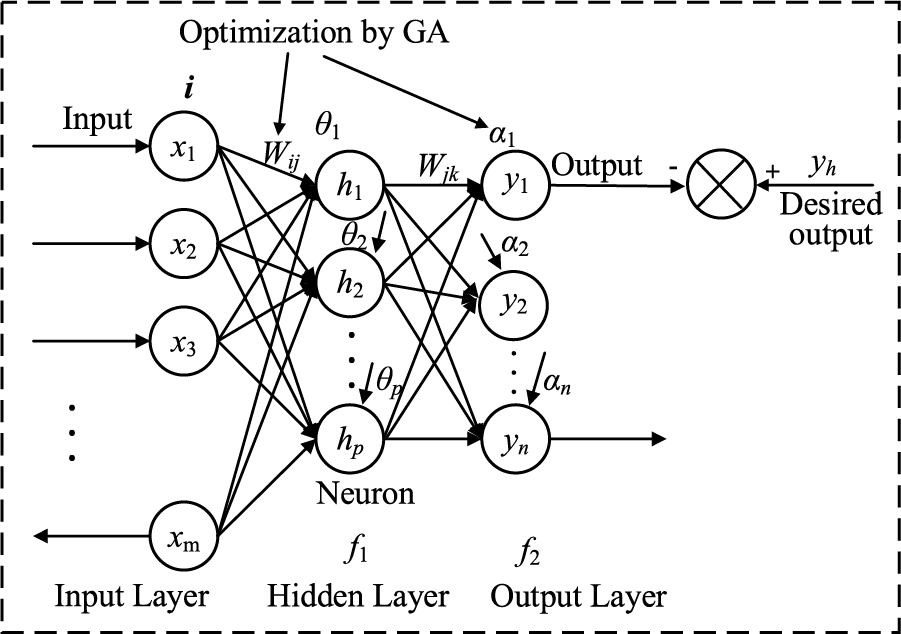
Figure 2: Structure of GA-BP network

LSTM network model is a type of deep neural network. LSTM solves the long-term dependency problem that recurrent neural network (RNN) cannot solve, that is, RNNs cannot learn long-distance dependencies in input sequences [25]. Moreover, LSTM enables models to selectively memorize effective data and delete invalid data, and solve the RNN problem of gradient explosion and gradient disappearance.

For a given sequence x = (x1, x2, ... , xn), the iterative calculation of the RNN structure is shown as follows:

ht=fa(Wxh∗xt+Whh∗ht−1+bh)(20)

yt=Why∗ht+by(21)

where W is Weight coefficient matrix; b represents Bias vector; fa denotes activation function.

LSTM unit includes the state of the memory unit and three gate control structures: forgetting gate, input gate, and output gate. Cell state is the pathway of information transmission, so that information can be transmitted in the sequence all the time. Theoretically, the cell state can transmit relevant information in the process of sequence processing all the time. As a result, earlier information can be transferred to later units, thus overcoming the lack of short-term memory. The addition and removal of information is accomplished through the gate structure, which has the function of judging and selecting to retain or forget information during training. The overall cell structure is shown in Fig. 3.

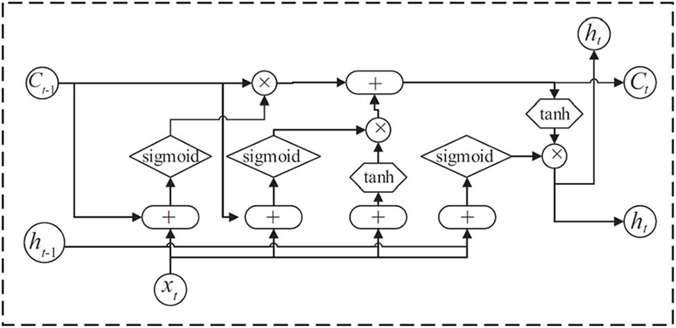
Figure 3: Long short-term memory hidden layer cell structure

LSTM solves the drawback of gradient disappearance and inflating of RNN by introducing a control gate, which makes the deep neural network developed in time easy to train. The forward calculation process is described by

it=η(Wxi∗xt+Whi∗ht−1+Wci∗ct−1+bi)(22)

ft=η(Wxf∗xi+Whf∗ht−1+Wcf∗ct−1+bf)(23)

ct=ftct−1+ittanh⁡(Wxc∗xt+Whc∗ht−1+bc)(24)

ot=η(Wxo∗xt+Who∗ht−1+Wco∗ct+bo)(25)

ht=ottanh⁡(ct)(26)

where i denotes input gate; f denotes forgotten gate; c represents cellular state; o is output gate; W means the corresponding weight coefficient matrix; b is the corresponding offset term; η denotes sigmoid activation function; tanh represents hyperbolic tangent activation function.

4.3 Forecasting Framework Based on ICEEMDAN-SE-LSTM Method

Based on the aforementioned discussion, this work constructs a forecasting model of wind power output based on seasonal classification. ICEEDAN wind power is used to decompose the wind power into a limited number of IMF, and then SE is used to classify and reconstruct the obtained IMF into three components. Then, the obtained components are input into LSTM to obtain the prediction results of each Subsequence, and the prediction results of each Subsequence are stacked to obtain the final prediction results. In the actual prediction process, the dataset suitable for LSTM model training is first constructed, and the data of environmental factors and wind power at time (t−1) are used to forecast the wind power value at time t. The wind power prediction framework proposed in this work mainly consists of four steps.

Firstly, the initial wind power historical data is processed as outliers, and then the annual datasets are classified into seasonal types according to the seasonal characteristics, and the prediction processing is carried out, respectively.

Secondly, ICEEMDAN is used for mode decomposition to address the non-stationary nature of wind power time series and the impact of high-frequency strong non-stationary components generated by traditional decomposition methods on prediction accuracy.

Thirdly, considering that there are too many sub-components after decomposition, the data processing is time-consuming and the training time is too long, SE is used to analyze the complexity of the obtained sub-components. The sub-components with correlation are reorganized into three groups with typical characteristics, i.e., trend component, oscillation component, and random component of wind power time sequence.

At the same time, the proposed model exists some limitations that can be further improved in future research. For instance, ICEEMDAN-based data processing will increase the data dimension, which leads to a longer prediction time for the data. Even if SE is used for sequence reconstruction, the data dimension is still higher than that before ICEEMDAN processing. Meanwhile, the prediction using LSTM is less effective for longer sequences and the prediction time is longer. In future research, the aforementioned two problems will be further analyzed and solved.

At the wind power prediction stage, an LSTM neural network that can fully explore the characteristics of time series is used for prediction, upon which wind power prediction curves under different seasons are finally obtained.

5  Case Studies

This study takes the measured wind power data of a wind farm with an installed capacity of 201 MW in Hami, Xinjiang Province from January 01, 2019, to December 31, 2019, as an example to analyze, and the sampling interval is 15 min. The annual data is divided into four groups based on four seasons, i.e., spring, summer, autumn and winter. The data collected on the last day of each season is used as the test data, and the rest is used as the training sample. The training sample is used to build the prediction model, and the test set is used to verify the prediction effect of the model.

To effectively assess the precision of proposed technique, this work chooses root mean squared error (RMSE), mean absolute error (MAE), and accuracy (Acc) as evaluation criteria. Particularly, RMSE, MAE, and Acc are calculated as following equations [7,8]:

ERMSE=∑t=1N(xp,t−xm,t)2N(27)

EMAE=∑t=1N|xp,t−xm,t|N(28)

Acc=(1−ERMSE)×100%(29)

where N is the number of test sample; xp,t represents the prediction value of wind generated power; xm,t denotes the actual power value of wind plant.

5.1 Mode Decomposition and Reconstruction Results of Wind Power Data

Firstly, the ICEEMDAN method is used to decompose the wind data sequence of four seasons, for example, the power sub-sequence components of each season are depicted in Fig. 4. The number of IMF decompositions in the four seasons are 6, 8, 9 and 11, respectively. The fluctuation of each IMF is different, that is, the IMF amount and waveform obtained after ICEEMDAN decomposition of wind power data in different seasons are different. Through ICEEMDAN decomposition, different time features of the initial power data in different seasons are extracted and reflected in different empirical mode components.

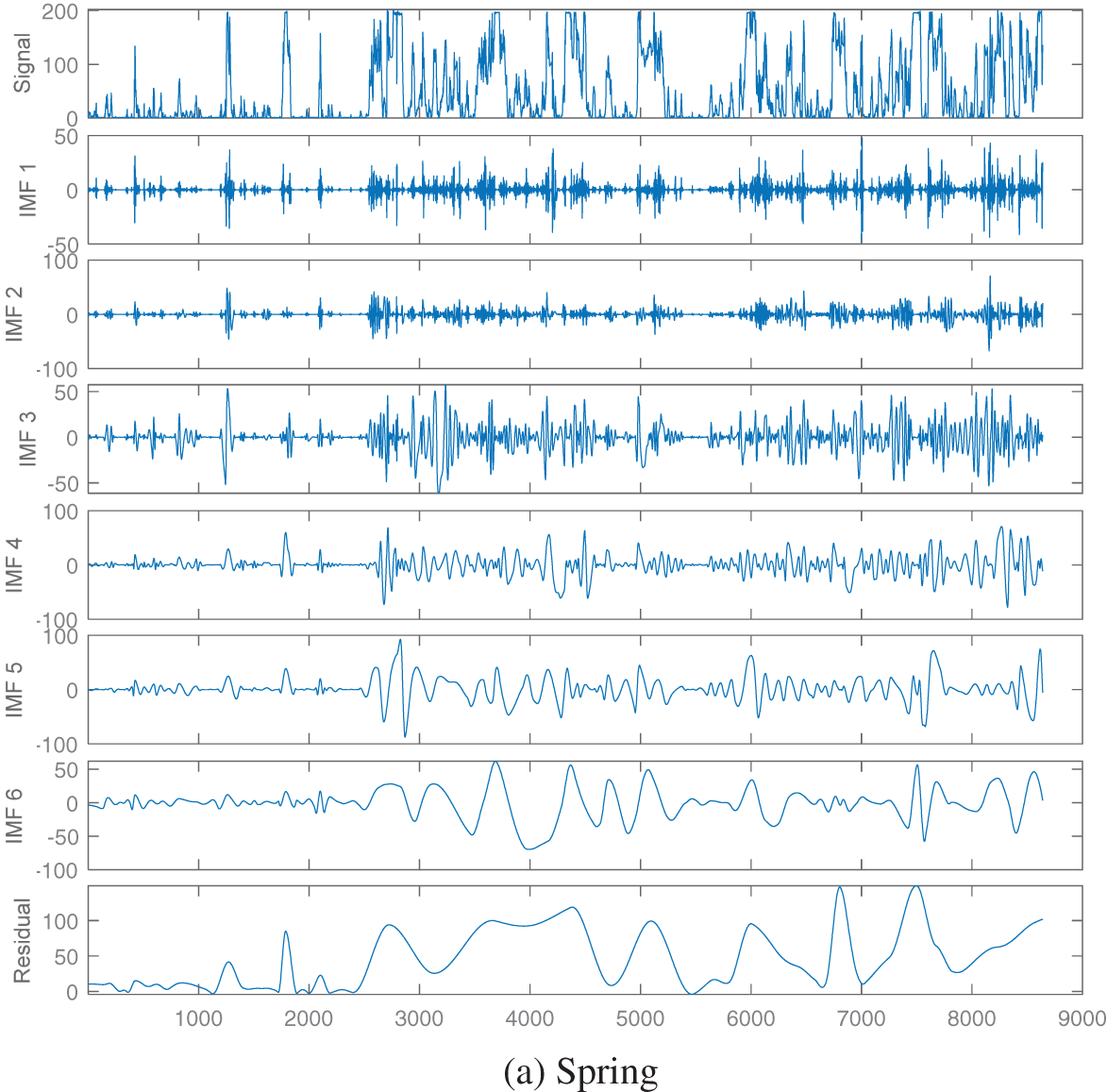
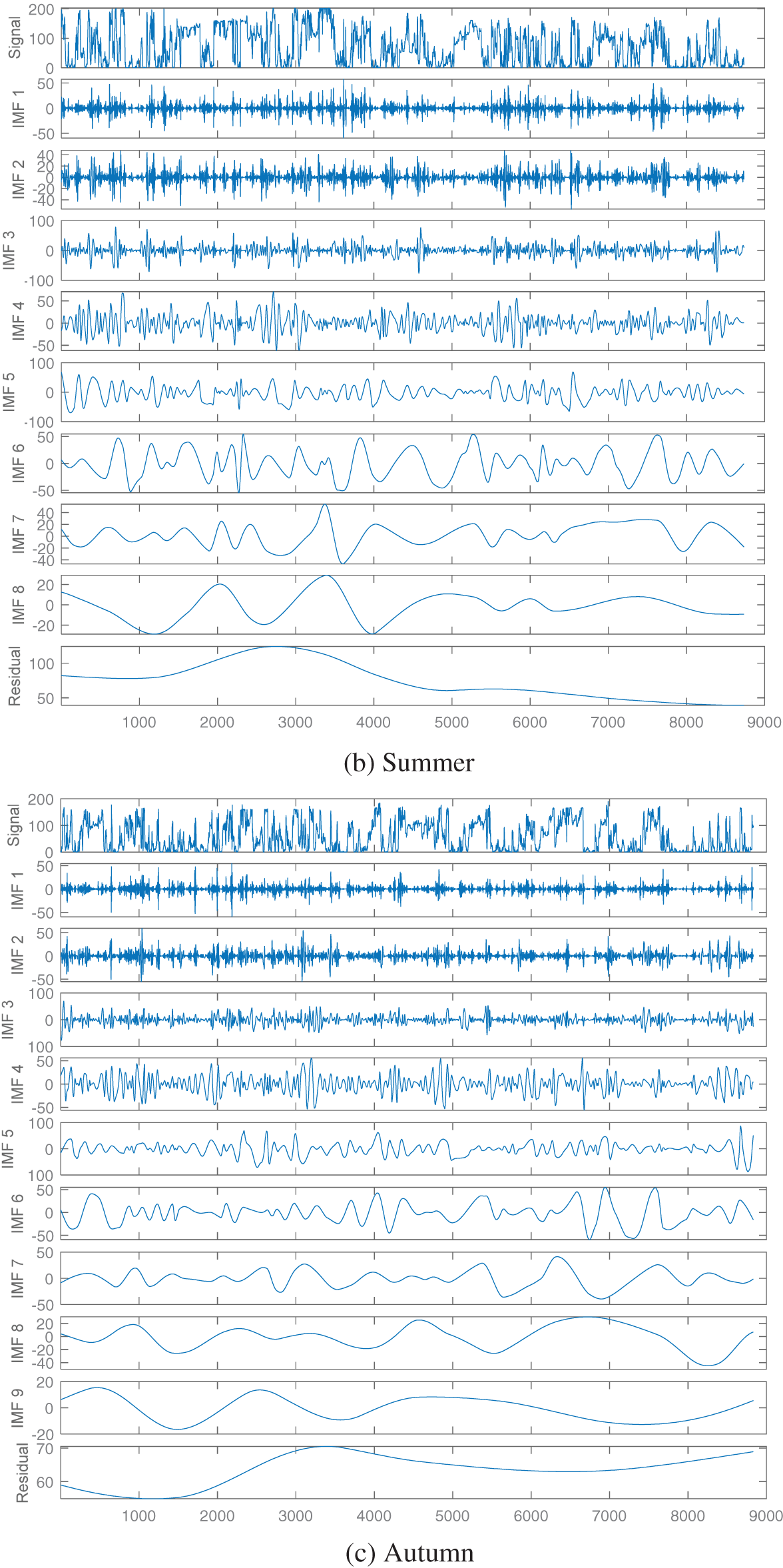
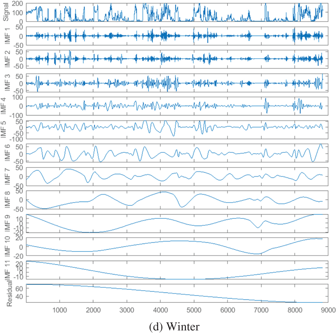
Figure 4: ICEEMDAN decomposition results of wind power sequence

In this study, the input power is decomposed into a power data sequence by ICEEMDAN, and the decomposed sequence is classified and reconstructed by SE. Then, three components are obtained, which replace the original power component as the input. As a result, wind speed, direction, temperature, atmospheric pressure, humidity, and power components are used as inputs to the model, while predicted power values are used as outputs.

Taking the IMF components reconstruction in the spring as an example, the order of the sub-components obtained from ICEEMDAN decomposition is recorded as sub-components 1–6.

The reconstructed components can roughly reflect the development trend of the driving force; Therefore, the reconstructed component is called the trend component. Similarly, sub-components 1 and 2 with similar sample entropy are reconstructed as random components, and sub-components 6 are taken as oscillatory components. The IMF components in summer are shown in Fig. 5b, and the order of the sub-components obtained from ICEEMDAN decomposition is recorded as sub-components 1–8. According to the sample entropy results in Fig. 5b, the sample entropy of sub-components 1, 2, and 8 are very close and can be reconstructed as trend components. Similarly, sub-components 4–6 with similar sample entropy are reconstructed as random components, and sub-components 3 and 7 are taken as oscillatory components. The reconstruction results in autumn and winter are shown in Figs. 5c and 5d.

Figure 5: Reconstruction result by SE

From the sample entropy results in Fig. 5a, it can be seen that the sample entropies of sub-components 3–5 are very close, indicating that their probability of generating new modes are basically the same, and they can be reconstructed as one component for prediction. The reconstructed component can roughly reflect the tendency of the original power; therefore, the reconstructed component is called the trend component. Similarly, sub-components 1 and 2 with similar sample entropy are reconstructed as random components, and sub-component 6 is taken as the oscillating component. IMF components under summer are shown in Fig. 5b, and the order of the sub-components obtained by ICEEMDAN decomposition is recorded as sub-components 1–8. According to the sample entropy result in Fig. 5b, the sample entropies of sub-components 1, 2 and 8 are close, which can be reconstructed into the trend component. Similarly, sub-components 4–6 with similar sample entropy are reconstructed as random components, and sub-components 3 and 7 are taken as oscillating components. The reconstruction results of autumn and winter are depicted in Figs. 5c and 5d.

5.2 Results Analysis of Simulation Test

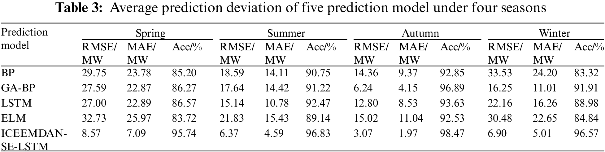
To demonstrate the effectiveness of the proposed model, a comparative analysis is conducted on the performance of BP, GA-BP, LSTM, ELM, and the proposed ICEEMDAN-SE-LSTM method. The GA-BP prediction model is a traditional prediction method employed to execute in parallel with ICEEMDAN-SE-LSTM. Based on components reconstruction, the wind power prediction curves of four seasons are shown in Figs. 6–9. Moreover, the prediction bias and accuracy of ICEEMDAN-SE-LSTM and GA-BP methods are tabulated in Table 2.

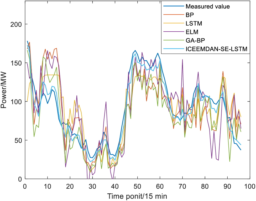
Figure 6: Wind power prediction results in spring

Figure 7: Wind power prediction results in summer

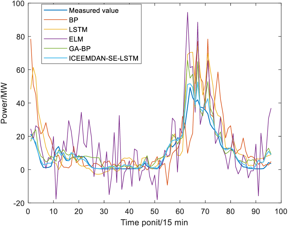
Figure 8: Wind power prediction results in autumn

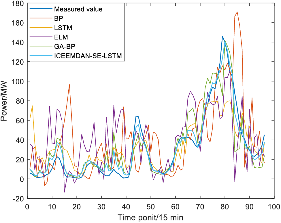
Figure 9: Wind power prediction results in winter

All the simulation tests are carried out based on MATLAB R2021b on a personal computer, with 32 GB of RAM and Intel (R) Core (TM) i5-9500 CPU @ 3.00 GHz as the processor.

Regarding the wind power prediction speed, the prediction time under all four seasons via this proposed method takes within 3 min, i.e., 179.86, 177.15, 176.28, and 175.54 s, respectively. The prediction generally aims at the output power of the next few hours or days, with a system data collection rate of 15 min. Even for real-time prediction, the prediction time of the proposed algorithm is still acceptable. Therefore, the running time of the proposed algorithm is able to meet the requirements of short-term power prediction.

From the perspective of data input dimension, the proposed model only processes the input power, while other inputs such as wind speed, wind direction, temperature, atmospheric pressure, and humidity are not processed by ICEEMDAN and their dimensions remain unchanged. In addition, the input dimensions are reduced by classifying and reconstructing the sequence using SE, which reconstructs the sequence components into trend components, oscillation components, and random components. Compared with other competitors, the increase in the input dimension of the proposed model is acceptable. In terms of running time, the prediction time for the four seasons achieves desirable results that all fall within 3 min. Therefore, compared with other algorithms, the proposed model has an increase in input dimensions, but its increase in model complexity is totally acceptable from the perspective of prediction time. For power prediction model evaluation, prediction accuracy is the first factor to be considered. Under the premise of acceptable prediction time, priority should be given to models with high prediction accuracy.

In spring, ICEEMDAN-SE-LSTM and GA-BP models both show poor prediction performance, with RMSE of 8.57 and 7.09 MW, and MAE of 27.59 and 22.87 MW, respectively. The reason may be that the dispersion degree of wind speed in spring is large and the fluctuation is violent, which leads to the difficulty of prediction. In autumn, the RMSE and MAE of the ICEEMDAN-SE-LSTM model are the smallest, with the value of 3.07 and 1.97, which might result from the value of wind speed in autumn being small and concentrated near the mean value, and the fluctuation range is not large. LSTM model is suitable for processing such time series with one-way time correlation and stable fluctuations. Due to the similarity in wind speed rhythms between summer and winter, the RMSE, MAE, and Acc indicators of both methods are approximate values.

The number of IMF based on ICIEMDAN decomposition varies in each season, with 6, 8, 9, and 11, respectively. The prediction accuracy for each season is 86.27%, 91.22%, 96.89%, and 91.91%, respectively. Meanwhile, based on the analysis of the five characteristic indicators of mean, variance, variable coefficient, asymmetry coefficient, and peak coefficient, the trend of spring wind speed is the steepest, with the highest and sharpest peak value. The trend of autumn wind speed is the smallest and most stable among the four seasons, while autumn and summer are relatively close and belong to medium. The number of IMF reflects the complexity of sequence data to a certain extent, but the results of power prediction are influenced by multiple factors, making it difficult to obtain a direct correlation between the number of IMF and prediction accuracy.

According to the results shown in Table 3 and Figs. 6–9, for the same prediction model, the prediction accuracy varies greatly among different seasons, with the best prediction results in autumn, followed by summer, winter, and spring. To be more specific, the Acc of the ICEEMDAN-SE-LSTM method in each season is 95.74%, 96.83%, 98.47% and 96.57%, respectively. In contrast, the Acc value for each season using the GA-BP method is 86.27%, 91.22%, 96.89% and 91.91%, respectively. In other words, the Acc of ICEEMDAN-SE-LSTM is higher than that of the GA-BP model ranging from 1.57% to 9.46%, which proves that the proposed method shows higher prediction accuracy.

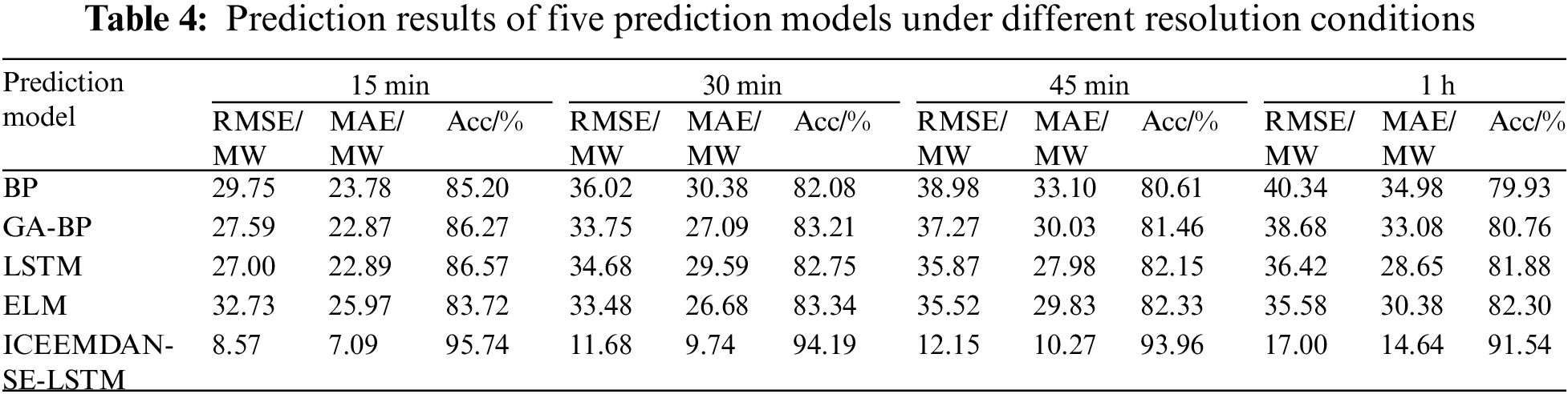
To verify the applicability of the proposed algorithm to data with different sampling rates, the original spring datasets are recollected at different resolutions of 15, 30, 45 min, and 1 h. The resulting data is predicted and analyzed using the data from the last day as the prediction dataset and the remaining data as the training dataset.

The prediction results of spring data at four different resolutions in Fig. 10 and Table 4 show that the proposed algorithm reached the highest accuracy, i.e., 95.74%, 94.19%, 93.96%, and 91.54% at resolutions of 15, 30, 45 min, and 1 h, respectively. In general, the proposed method can achieve higher than 91% accuracy under all four different resolutions, further validating its strong applicability and high prediction accuracy.

Figure 10: Spring wind power prediction results with different resolutions

6  Conclusion

Due to the strong uncertainty of wind speed series, the fluctuations in wind power vary with seasons. To enhance the prediction accuracy of output wind power, a wind power day-ahead forecasting method based on the ICEEMDAN-SE-LSTM model is established in this work. Its main contributions are drawn as follows:

(1) For wind power data processing, ICEEMDAN decomposition and sample entropy technology can effectively reduce the adverse effects of high-frequency and strong non-stationary components in the original data series, upon which favorable conditions can be constructed to improve model prediction performance while simplifying the model;

(2) The variation of wind speed in different seasons is not the same, thus its mapping relationship in prediction models is also different. Autumn has the highest prediction accuracy for the two models, followed by summer, winter and spring, with the accuracy of the proposed method reaching 95.74%, 96.83%, 98.47% and 96.57%, respectively, which verifies the effectiveness of ICEEMDAN-SE-LSTM model;

(3) ICEEMDAN-SE-LSTM and other methods are utilized to forecast the wind power in parallel for comparison, and the simulation results indicate that the ICEEMDAN-SE-LSTM method shows higher prediction precision than the traditional models;

(4) The model proposed in this study relies on the proper integration of existing mature technologies to realize power prediction of wind farms actually operating in Xinjiang, China. Compared with EMD, ICEEDAN-based data analysis is more capable of mining wind power data features and improving wind power prediction accuracy. Meanwhile, SE is utilized to classify and reconstruct the multiple ordinal components processed by ICEEDAN into trend, oscillation, and stochastic components, which reduces the data dimensionality and improves the prediction speed. The hybrid model is used to compensate for the low prediction accuracy of a single LSTM model. Compared with other comparison algorithms, the proposed model shows superior performance in terms of stability, reliability, and accuracy requirements of engineering practice.

Future studies can further increase the input characteristic dimension based on the current work, and input the numerical weather forecast and other related information into the prediction model to further improve the prediction precision.

Acknowledgement: Thank you very much for the support provided by State Grid Shandong Electric Power Company for this paper.

Funding Statement: This work is supported by Science and Technology Project of State Grid Shandong Electric Power Company (52062622000R, Research on Aggregation and Regulation Technology of Regional Integrated Energy System).

Author Contributions: The authors confirm contribution to the paper as follows: study conception and design: Shumin Sun, Peng Yu; data collection: Jiawei Xing; analysis and interpretation of results: Shumin Sun, Yan Cheng; draft manuscript preparation: Song Yang, Qian Ai. All authors reviewed the results and approved the final version of the manuscript.

Availability of Data and Materials: All data comes from Xinjiang, China, and according to data confidentiality requirements, the data used cannot be disclosed.

Conflicts of Interest: The authors declare that they have no conflicts of interest to report regarding the present study.

References

1. Yang, B., Zhong, L., Wang, J., Shu, H., Zhang, X. et al. (2021). State-of-the-art one-stop handbook on wind forecasting technologies: An overview of classifications, methodologies, and analysis. Journal of Cleaner Production, 283, 124628. [Google Scholar]

2. Jung, J., Broadwater, R. P. (2014). Current status and future advances for wind speed and power forecasting. Renewable and Sustainable Energy Reviews, 31, 762–777. [Google Scholar]

3. Song, D., Yang, J., Fan, X., Liu, A., Chen, J. et al. (2018). Maximum power extraction for wind turbines through a novel yaw control solution using predicted wind directions. Energy Conversion and Management, 157, 587–599. [Google Scholar]

4. Kazem, H. A., Yousif, J. H. (2017). Comparison of prediction methods of photovoltaic power system production using a measured dataset. Energy Conversion and Management, 148, 1070–1081. [Google Scholar]

5. Liu, C., Zhang, X., Mei, S., Liu, F. (2021). Local-pattern-aware forecast of regional wind power: Adaptive partition and long-short-term matching. Energy Conversion and Management, 231, 113799. [Google Scholar]

6. Guchhait, P. K., Banerjee, A. (2020). Stability enhancement of wind energy integrated hybrid system with the help of static synchronous compensator and symbiosis organisms search algorithm. Protection and Control of Modern Power Systems, 5(1), 11. [Google Scholar]

7. Yu, G., Liu, C. Q., Tang, B., Chen, R., Lu, L. et al. (2022). Short term wind power prediction for regional wind farms based on spatial-temporal characteristic distribution. Renewable Energy, 199, 599–612. [Google Scholar]

8. Wang, J., Song, Y., Liu, F., Hou, R. (2016). Analysis and application of forecasting models in wind power integration: A review of multi-step-ahead wind speed forecasting models. Renewable and Sustainable Energy Reviews, 60, 960–981. [Google Scholar]

9. Ambach, D., Schmid, W. (2017). A new high-dimensional time series approach for wind speed, wind direction and air pressure forecasting. Energy, 135, 833–850. [Google Scholar]

10. Liu, D., Niu, D., Wang, H., Fan, L. (2014). Short-term wind speed forecasting using wavelet transform and support vector machines optimized by genetic algorithm. Renewable Energy, 62, 592–597. [Google Scholar]

11. Wang, Y., Zou, R., Liu, F., Zhang, L., Liu, Q. (2021). A review of wind speed and wind power forecasting with deep neural networks. Applied Energy, 304, 117766. [Google Scholar]

12. Wu, Z., Luo, G., Yang, Z., Guo, Y., Li, K. et al. (2022). A comprehensive review on deep learning approaches in wind forecasting applications. CAAI Transactions on Intelligence Technology, 7(2), 129–143. [Google Scholar]

13. Sun, M., Feng, C., Zhang, J. (2019). Conditional aggregated probabilistic wind power forecasting based on spatio-temporal correlation. Applied Energy, 256, 113842. [Google Scholar]

14. Fan, L., Wei, Z., Li, H., Kwork, W. C., Sun, G. et al. (2017). Short-term wind speed interval prediction based on VMD and BA-RVM algorithm. Electric Power Automation Equipment, 37(1), 93–100. [Google Scholar]

15. Wang, Y., Wang, Z., Huang, M., Yang, M. (2014). Ultra-short-term wind power prediction based on OS-ELM and bootstrap method. Automation of Electric Power Systems, 38(6), 14–19. [Google Scholar]

16. Wang, B., Liu, C., Zhang, J., Feng, S., Li, Y. et al. (2015). Uncertainty evaluation of wind power prediction based on Monte-Carlo method. High Voltage Engineering, 41(10), 3385–3391. [Google Scholar]

17. Yin, H., Zeng, Y., Meng, A., Yang, L. (2018). Wind speed multi-step interval prediction based on singular spectrum analysis-fuzzy information granulation and extreme learning machine. Power System Technology, 42(5), 1467–1474. [Google Scholar]

18. Sun, R., Zhang, T., He, Q., Xu, H. (2021). Review on key technologies and applications in wind power forecasting. High Voltage Engineering, 47(4), 1129–1143. [Google Scholar]

19. Lu, P., Ye, L., Zhao, Y., Dai, B., Pei, M. et al. (2021). Feature extraction of meteorological factors for wind power prediction based on variable weight combined method. Renewable Energy, 179, 1925–1939. [Google Scholar]

20. Li, C., Peng, X., Wang, H., Che, J., Wang, B. et al. (2022). Short-term power prediction of wind power cluster based on SDAE deep learning and multiple integration. High Voltage Engineering, 48(2), 504–512. [Google Scholar]

21. Hong, Y., Rioflorido, C. L. P. P. (2019). A hybrid deep learning-based neural network for 24-h ahead wind power forecasting. Applied Energy, 250, 530–539. [Google Scholar]

22. Lin, Z., Liu, X., Collu, M. (2020). Wind power prediction based on high-frequency SCADA data along with isolation forest and deep learning neural networks. International Journal of Electrical Power & Energy Systems, 118, 105835. [Google Scholar]

23. Zhang, X., Liang, J., Zhang, X., Zhang, F., Zhang, L. et al. (2013). Combined model for ultra short-term wind power prediction based on sample entropy and extreme learning machine. Proceedings of the CSEE, 33(25), 33–40 (In Chinese). [Google Scholar]

24. Kang, T., Qin, Z. (2022). An ultra-short-term wind power forecasting method based on hyperparameter optimization and dual-stage attention mechanism. Southern Power System Technology, 16(5), 44–53. [Google Scholar]

25. Greff, K., Srivastava, R. K., Koutník, J., Steunebrink, B. R., Schmidhuber, J. (2017). LSTM: A search space odyssey. IEEE Transactions on Neural Networks and Learning Systems, 28(10), 2222–2232. [Google Scholar] [PubMed]