Prediction Model of Drilling Costs for Ultra-Deep Wells Based on GA-BP Neural Network

1  Introduction

As the development of oil and gas exploration going on, it aims to do the operation in deep and ultra-deep layers, which makes petroleum projects more and more complicated. Through the experience of development projects, it shows the following characteristics: large investment, low return, and high risk [1,2]. Facing the problem of rising total investment, how to reduce cost and promote efficiency is the key concern of enterprises now. In order to maximize the net present value (NPV) of oil and gas development, it has better to start optimization as early as in the design and planning of oil and gas development. The accuracy of cost estimation is directly related to the accuracy of the technical and economic evaluation results. The accuracy of its drilling costs has a significant impact on the subsequent investment decisions and design of strategy development [3,4].

In the past, drilling costs forecasting methods were mostly based on traditional statistical models such as regression models and gray models. Statistical prediction methods estimate the values of model parameters by sample data with known equation structure and the number of parameters, which is called parametric regression. Kaiser et al. created generalized functional models for drilling cost estimation. Well characteristics, well complexity, site characteristics, operator preference and other features were considered. As a result, the average dry hole days and dry-hole cost regression equations are given [5]. Kitchel et al. estimated drilling cost through probabilistic model. In that model, risk-analysis program and drilling cost forecasting were combined. The Monte Carlo simulation was used to do the risk analysis job [6]. There is no comprehensive equation in that model, and the excel spreadsheet was used to do all steps of calculation and simulation. In other words, this is an analysis system rather than an explicit equation. Shilling et al. [7] created a system to estimate and track drilling authorization for expenditure (AFE) cost automatically. On average, the system could provide an estimated cost with 20%−30% difference with the actual drilling booked cost in the historical test [7]. Rodriguez presented a way to estimate time and costs for the drilling project in the Tapir Field. Well characteristics, drilling information involving average ROP, time spent on each trip et al. were collected [8]. The excel spreadsheet was used to complete all calculation. In the real-life application, the estimation error is only $0.5 MM. Akins et al. provided probabilistic model to estimate drilling time and costs. The probabilistic model was operated through the defined distribution of drilling features and Monte Carlo simulation [9]. Although this model is applied in the three case wells successfully, it cannot eliminate the subjectivity. In other words, the potential relationship between drilling cost and features is still controlled by the experience of human beings. Ugochukwu estimated the intervention operations cost in subsea through the risk analysis and probabilistic methods. The difference between the estimation cost and the actual cost is less than 7% [10].

Although traditional and statistical methods of drilling cost estimation is popular, there are several weaknesses of it. Firstly, the regression method is one of the parametric methods. The regression equation is set before training. The goal of training is to find appropriate coefficients. It is a limitation to find the potential non-linear relationship between features and output. Secondly, the regression method represents that the number of drilling cost features is limited, or the dimensional reduction method has to be applied to eliminate the features. More or less, the information would be lost after this operation. Thirdly, the traditional cost estimation system involves the experience of drilling operator, and it means that there is subjective influence on the estimation. In summary, it is difficult to meet those premises to make result appropriate to consider alternative methods to estimate drilling costs with as little error as possible.

Artificial neural network methods, optimization algorithms and their hybrid models have been shown to be powerful in function approximation, especially in the drilling cost estimation. Moreover, these methods can withstand a wide range of uncertainties. According to this idea in the related field has been studied by domestic and foreign scholars in related fields, and certain progress has been made. Zhao et al. used a Bayesian regularized neural network to predict drilling costs [11]. Five different kinds of cost categories were considered in that model, and well structure factors are also involved. Different algorithms were compared to test the model’s generalization ability. Guo et al. used four artificial intelligence techniques, artificial neural network (ANN), random forest (RF), support vector machine (SVM), and classification and regression trees, to estimate the mining capital cost of an open pit copper mining project with high accuracy [12]. In that study, the ANN shows the best performance with the most dominant accuracy. In detail, RMSE is 138.103, R2 is 0.99, MAE is 114.589 and APE is 7.77%. Zheng et al. developed a novel cascaded forward neural network-based optimization model to predict mining capital costs by exploring the relationship between factors of production, ore grade, and mine life [13]. In the optimization algorithm named slap swarm, is used to tuning the machine learning model, which could improve machine learning model’s efficiency and performance. It is a common method to find the optimization of hyperparameters of machine learning model. Neural networks have been used in mining cost estimation [14]; however, some scholars have reported that using back propagation (BP) algorithms to tune the parameters of neural networks has some drawbacks, such as slow learning speed and getting trapped in local optimal solution. Using evolutionary algorithms to train neural networks instead of traditional (e.g., BP) algorithms alone could have the effect of improving prediction performance [15].

In current paper, a back-propagation neural network optimized by GA to predict drilling costs is given, and it is based on dissecting the cost components of ultra-deep wells and the actual dominant factors of drilling cost. The structure of the current paper is that the methodology would be given first. The flowchart, BP algorithm, GA optimization algorithm will be introduced in that section. Next, it is the feature selection section. Data preprocessing and the dominant factor analysis will be given in that section. Results and discussion section is following section. The performance of the hybrid model will be shown. Lastly, the conclusion would be given.

2  Methodology

2.1 BP Neural Network for GA Optimization

BP neural networks are sensitive to the initial connection weights between the input layer and the hidden layer, the hidden layer and the output layer neurons, and the initial bias of the hidden layer and the output layer. However, the initial weights and bias in BP neural networks are randomly designated without any scientific basis. The result is that those two factors could affect the accuracy when training.Therefore, the current paper applies the genetic algorithm (GA) to optimize the initial weights and bias of the BP neural network. Specifically, the following operations are included (Fig. 1):

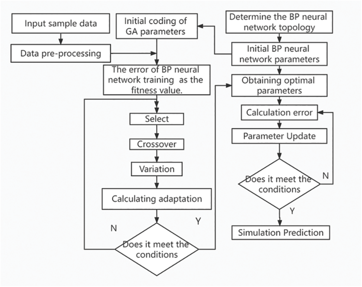
Figure 1: Flowchart of the optimized BP neural network of GA

Step 1 Determine the BP neural network topology.

Step 2 Determine the BP initialization hyper-parameters, including the learning rate, the number of layers in the hidden layer, the number of nodes in the hidden layer, the momentum factor, the activation function, etc.

Step 3 Determine the GA initialization parameters, including the maximum number of genetic generations, population size, crossover probability, and variation probability, and select the fitness function.

Step 4 Perform a binary number to encode a representation of the initial network weights and bias.

Step 5 Continuous optimization of network weights and bias based on the basic operations of replication, crossover and mutation of the GA.

Step 6 Determine whether the weights and bias are optimal, and if not, repeat Step 5 until the optimal solution is found.

Step 7 Assign the optimal solution from Step 6 to the BP neural network.

2.2 BP Neural Network

Back propagation neural network (BP) is a machine learning model that mimics the structure of biological neural networks. The BP neural network learns the parameters of the neural network by forward propagation of information and backward propagation is to correct the training error [16]. The known information goes into the whole network through the input layer, and then process it in the hidden layer, finally, the output value is shown as output, which is known as forward propagation of information. The process of error back propagation is done by calculating the error between the actual output and the desired output to correct the connection weights of the whole network and the bias of each node in each layer. The training of the entire neural network is completed when the error convergence is stopped at a minimum. Fig. 2 shows the schema of the BP neural network.

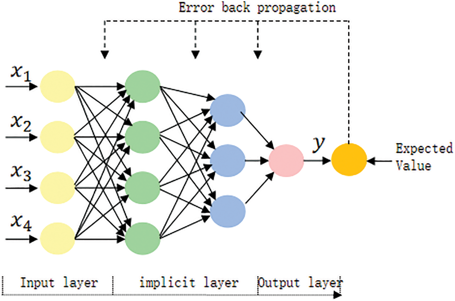
Figure 2: Schema of neural network

The training process of BP neural network is:

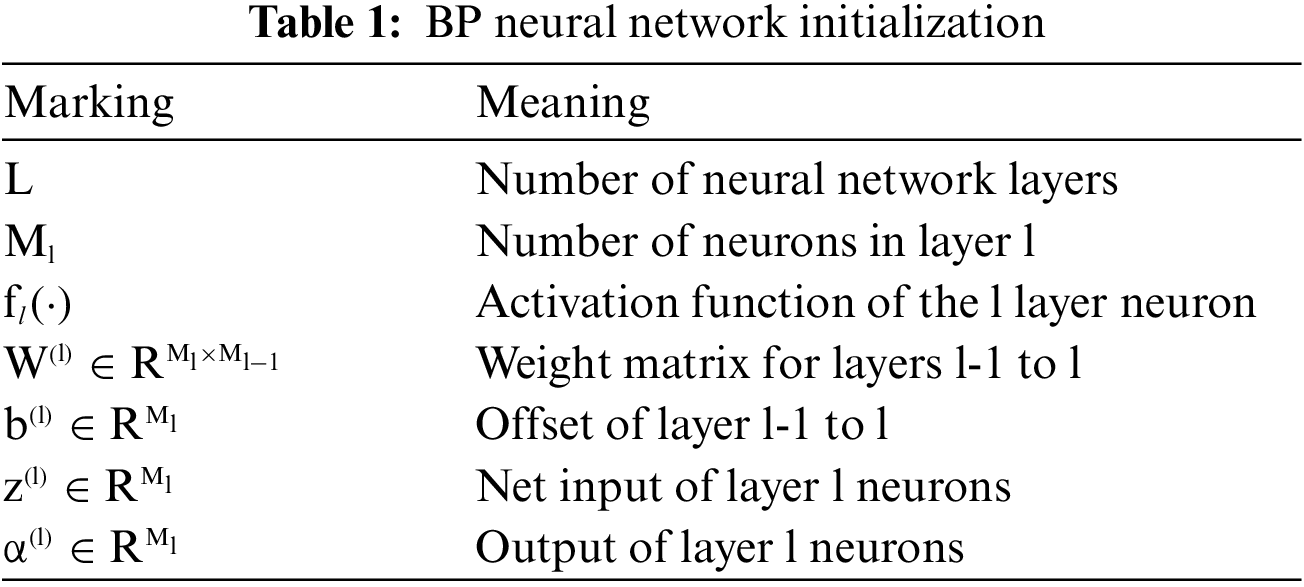
(1) Initialization

BP neural network initialization parameters are shown in Table 1.

The S-type function Sigmoid function is selected as the activation function between the layers in the neural network, which maps the signal non-linearly into the (0,1) interval. The formula is:

f(x)=11+e−x(1)

(2) Forward propagation

The lth layer neuron is passed through its input layer to the hidden layer, where the weighted sum is calculated, which is the sum of each input value multiplied by its weight vectors, and then added by the bias. The formula is:

z(l)=W(l)α(l−1)+bl(2)

The output value of the hidden layer of the lth layer neuron is obtained by inputting the above-derived result into the activation function to obtain the output of the lth layer neuron. The calculation formula is:

α(l)=fl(z)(l)(3)

(3) Back propagation

According to the chain rule, gradient descent is used to update the parameters in the network. The training set is D={(x(n),y(n))}n=1N, the desired output result is y(n), the validation set is V, the regularization factor is λ, the number of network layer is L, the number of neurons is Ml,1≤l≤L.

Calculate the error for each layer:

δ(l)=∑n=1Ml(y^(n)−y(n))22(4)

Find the derivatives of the parameters at each level:

∀l,∂ζ(y(n),y^(n))∂ω(l)=δ(l)(α(l−1))T (5)

∀l,∂ζ(y(n),y^(n))∂b(l)=δ(l)(6)

According to the above method the parameters are updated, and the error is continuously calculated. If the error rate of the neural network on the validation set no longer decreased, the output will be given based on the newest W,b. The whole training process of the BP neural network is completed.

2.3 BP Neural Network

Genetic Algorithms (GA) is a search (optimization) algorithm based on the principles of natural selection and natural genetic mechanisms, which simulates the evolutionary mechanisms of life in nature to achieve optimization of a specific goal in an artificial system. The essence of GA is to evolve generation by generation according to the principle of survival of the fittest by means of population search technique to finally obtain the optimal solution or quasi-optimal solution.

We use decimal coding, and the optimization processes are as follows:

(1) Population initialization. All the weights and biases of the neural network model are used to establish the population information, and the weights and biases are cascaded in a certain order equivalent to a chromosome. Its length is:

L=N(N+O)+Y+O(7)

where L is the chromosome length; N is the number of input nodes; O is the number of output nodes; Y is the number of hidden layer nodes.

(2) Individual fitness calculation. The optimal chromosome for each evolutionary generation in the population is found by calculation and recorded for retention. The fitness function chosen in this paper is:

F(i)=1∑i=1n(y^(i)−y(i))2(8)

where n is the number of samples, and y^(i) and y(i) are the simulated and measured values of the samples, respectively.

(3) Genetic evolution. The genetic overlapping generation operations of selection, crossover, and mutation, and individual adaptation calculation are cyclically performed.

(4) To obtain the highest individual adaptation combination.

3  Feature Selection

3.1 Cost Analysis of Drilling in Ultra-Deep Well

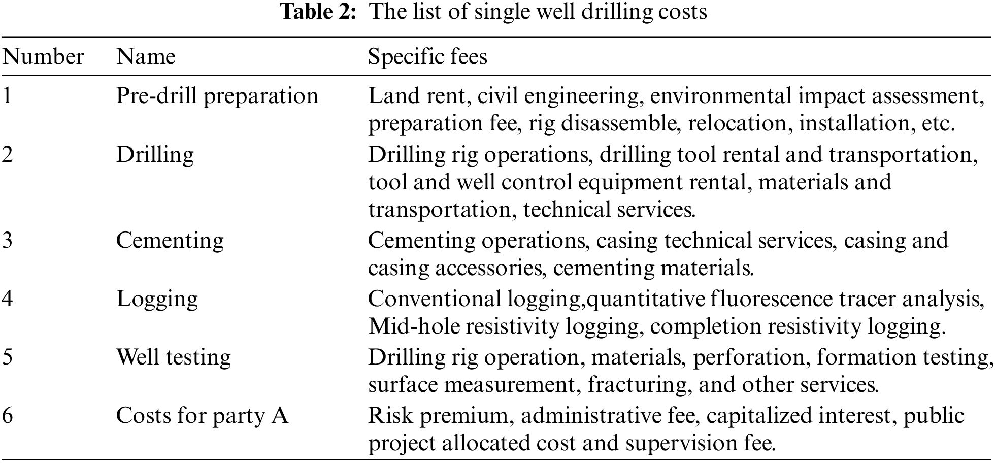
Characteristics of the drilling and completion operations of deep/ultra-deep wells are to work under the complex geological conditions, and lack of mature technology, which leads to high total drilling and completion costs. As the development depth being much greater than before, each well shows the completely different operation conditions, which makes drilling and completion costs forecasting extremely difficult [17]. Drilling costs is calculated, which involves the pre-drilling preparation to the end of the well testing and installation of the oil recovery wellhead of single well. The total cost covers pre-drilling preparation, drilling, cementing, logging, and well testing [17–19]. In the previous five major individual work, different stages of production would generate a variety of costs. Individual projects and cost components are shown by Table 2.

3.2 Drilling and Completion Cost Dominant Factors

Drilling and completion are a complex system engineering that subject to many factors, and its cost is affected by many factors. Although the equipment and tools of the same operation unit are definite, the judgement of the drilling operator and the formation conditions are random, which makes the uncertainty of drilling costs. Analysis of the drilling data shows the following relationships between drilling and completion costs and their dominant factors:

(1) Well depth. The greater the footage, the higher the drilling costs, and conversely, the less footage, the lower the drilling costs.

(2) Operating period. The longer the operation, the higher the direct and amortized costs of labor, machinery, depreciation, etc.

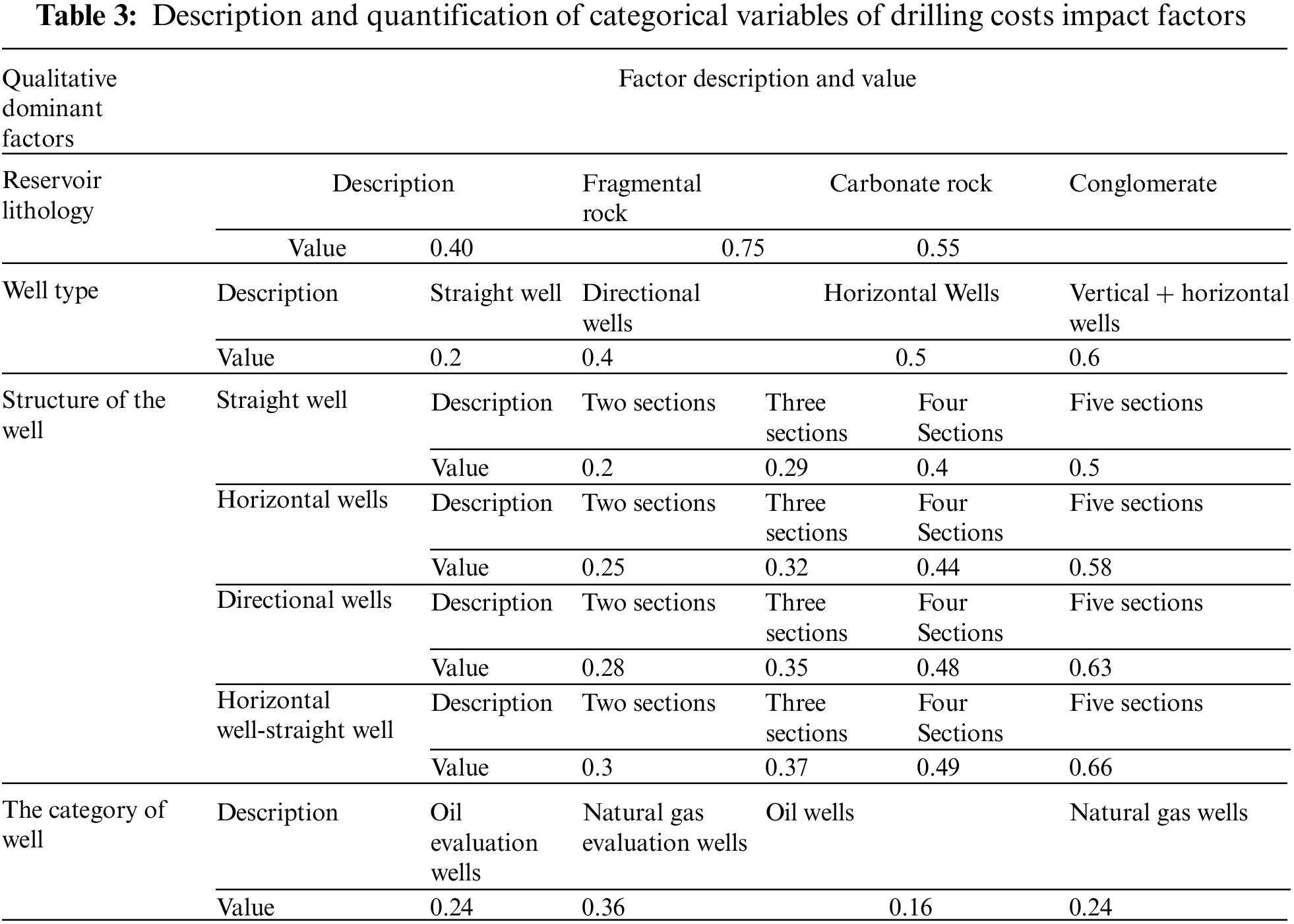
(3) Lithology of the reservoir. The tighter the lithology, the longer the operating period and the higher the drilling costs. Conversely, the shorter the drilling period, the lower the drilling costs.

(4) Well type. Including straight wells, directional wells, and horizontal wells, well types differ and so do the quotas for drilling costs.

(5) Well structure. Different well structures require different materials such as casing and wellhead devices, resulting in different drilling costs.

(6) Category of well. Wells are generally divided into gas development wells, oil development wells, gas exploration wells and oil exploration wells. Factors, like that the operation of geological coring obtain and unfamiliarity with the geology makes the cost of exploratory wells is higher than the cost of development wells, meanwhile, the cost of gas wells higher than the cost of oil wells.

3.3 Data Pre-Processing

3.3.1 Data Acquisition

Basic data in 2019–2021 for drilling costs forecasting analysis of the oil field was collected, including reservoir lithology, well type, well structure, well category, well depth, drilling cycle and drilling costs. It consists of 119 data samples covering drilling depths above 4,500 meters (4,500–8,500 meters). The data obtained are separated into categorical variables and numerous variables. Categorical variables, including reservoir lithology, well type, well structure et al. Numerical variables include well depth, drilling period and drilling costs. Box plots shows the observation of the feature distribution. Pearson correlation coefficients is calculated to investigate the linear relationship between well depth, drilling period and drilling costs.

3.3.2 Categorical Variable Analysis

Based on the actual situation of drilling operations and the opinions of professional staff, normalized descriptions and quantified (including normalized) values of drilling costs impact factors are given [20]. The description and quantification results of the categorical variables of drilling costs dominant factors for the T oilfield samples are shown in Table 3.

3.3.3 Numerical Variables

The box plot (Fig. 3) shows the distribution of well depth, drilling period and drilling costs. The distribution is relatively uniform, the average drilling period is about 200 days, and drilling costs concentrates on the lower quarter of the box. There are a few outliers in the drilling period and drilling costs graph, and those sample points are removed manually.

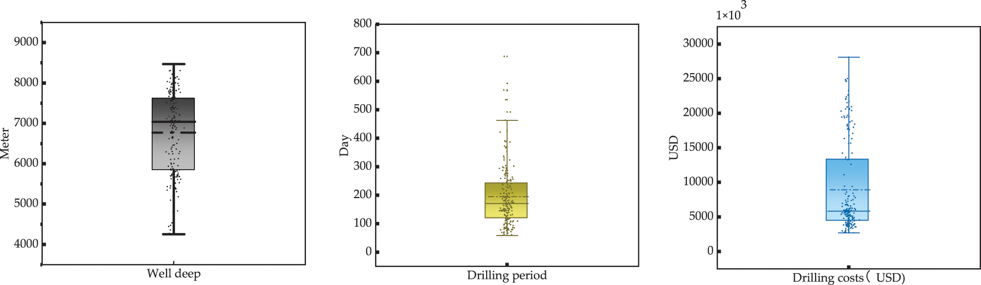
Figure 3: Distribution of well depth, drilling cycle and drilling costs data

The correlation between well depth, drilling period and drilling costs is analysed to investigate the feasibility of artificial intelligence models to predict drilling costs. Pearson correlation coefficients (abbreviated as R2) and p-values were calculated for drilling period and drilling costs, and R2 and p-values were calculated for well depth and drilling costs correlation coefficients, and scatter plots and correlation coefficients are shown in Figs. 4 and 5. Based on the visualization and coefficients in Figs. 4 and 5, it is clear that the p-value is <5% and the correlation between well depth, drilling period and drilling costs is significant and the correlation is high enough to consider using an artificial intelligence model to predict drilling costs.

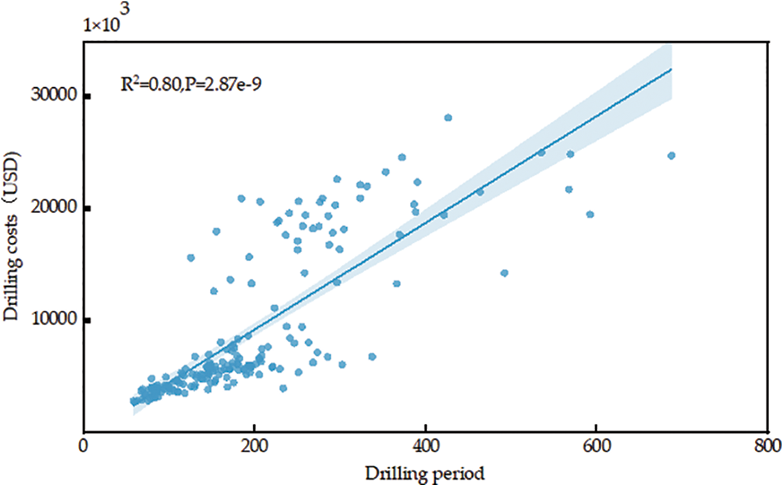
Figure 4: Correlation between drilling period and drilling costs

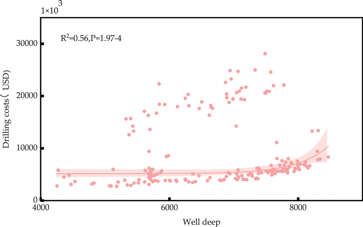
Figure 5: Correlation between well depth and drilling costs

3.3.4 Data Normalization

The units of the indicators of the influencing factors of drilling costs are different, while the values of each factor vary greatly. In order to avoid the influence of inconsistencies in the scale and differences in values on the analysis of mining costs, the data of the influencing factors of drilling costs are standardized using the polarization method. The normalization formula:

xnorm=xi−xminxmax−xmin(9)

The parameter values are normalized to the interval [0, 1]. xi is ith value of sample before normalization; xnorm is the value after normalization; xmax, xmin are the maximum and minimum values of the data before normalization, respectively.

3.4 Drilling Costs Prediction Model

The 6 features are used as input and the drilling costs are used as output. There are 136 samples in total, and 100 of them were chosen randomly to do the training and validation task. In detail, the ratio between training and validation is 7:3. The rest of original data set works as test data set, which is used for evaluating the prediction model. BP neural networks have direct connections from the input to the hidden and output layers. This kind of model can represent the nonlinear relationship between the input and output. To avoid over-fitting, a single hidden layer is chosen, a Sigmoid function is activation function, and the loss function is Levenberg-Marquardt. The optimal node value range of the hidden layer is set to be [10,20]. Furtherly, the number of optimal nodes is determined to be 7:12:1 by trying multiple times network training. The maximum number of epochs is set to be 1,000; the learning rate is 0.01; the target error of input and output is 0.001. Based on those, a GA with global search capability is introduced to optimize the weights and bias of BP neural network. The GA parameters were set to be a maximum genetic generation of 20, a population size is 10, a crossover probability is 0.3, and a variance probability is 0.1. The sum prediction error of the neural network was used to be the adaptation function.

4  Results and Discussion

4.1 Figures

Matlab software is applied in this paper, and the training results is shown by Fig. 6. As the number of iterations increases, the GA algorithm adaptation curve gradually decreases, and the optimal individual adaptation reaches the minimum value after 17 generations of population evolution in the process of continuous iterative evolution, indicating that the population has reached steady state. Fig. 7 shows the prediction errors of the GA-BP network in the training set, and it can be seen that most of the errors are concentrated in the range of ±8%. The weight of the training set error within ±10% was statistically calculated to be 94%. Fig. 8 shows the prediction effect of drilling costs corresponding to 36 test sets of data. It can be seen that the proposed model can predict the output variables very well.

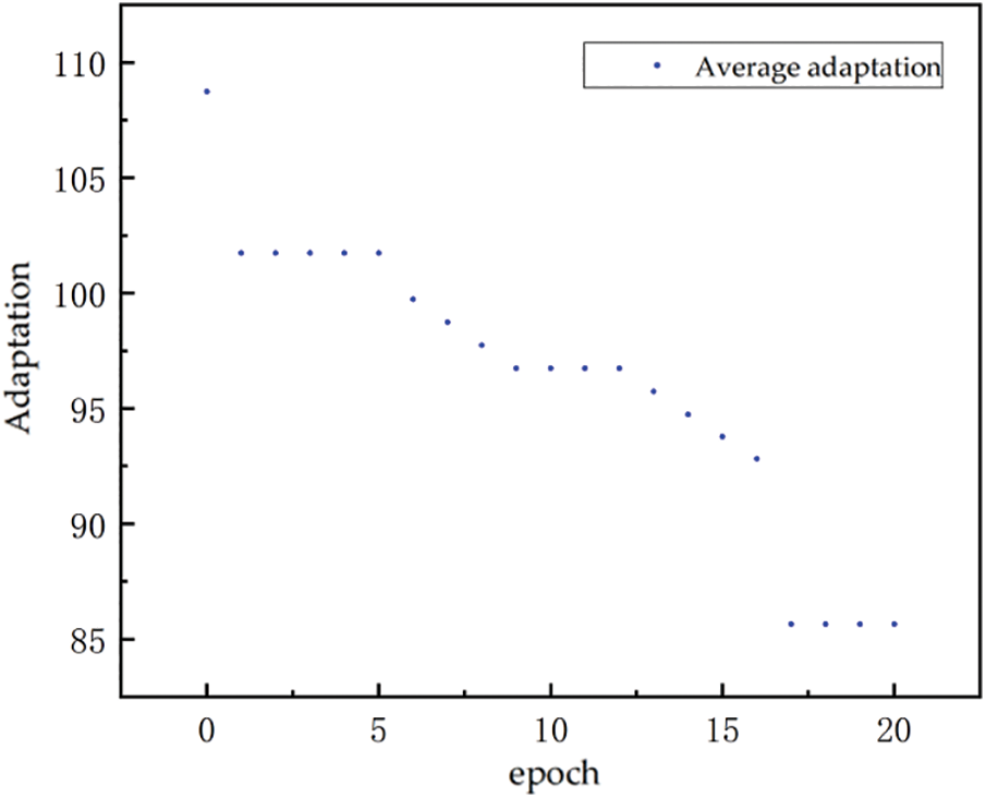
Figure 6: GA algorithm adaptation curve

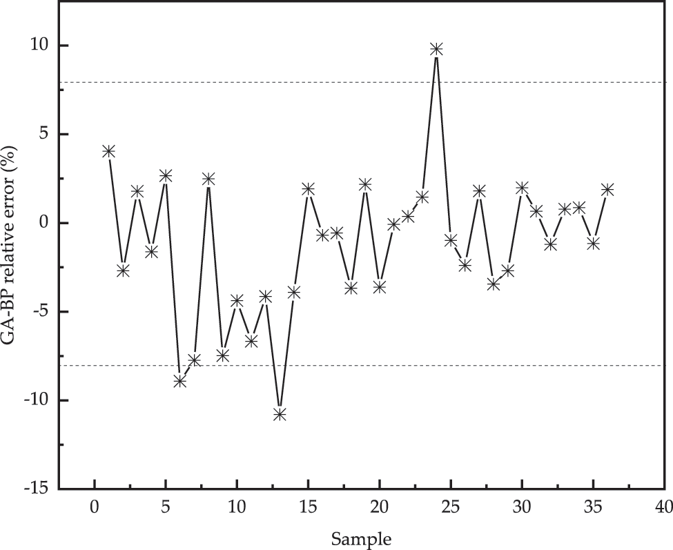
Figure 7: Prediction error of GA-BP network in training set

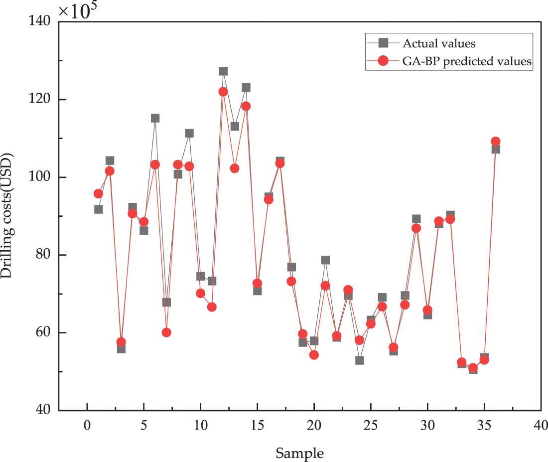
Figure 8: GA-BP model test set data corresponding to the drilling costs prediction results

In order to test the effectiveness of the GA algorithm to optimize the BP neural network, the comparison between the proposed hybrid model and the base BP neural network model. In order to visualize the advantages of the GA-BP method. The predicted values of the test data of the two methods were selected for comparison, as shown in Fig. 9. As can be seen from Fig. 9, the traditional BP neural network model can also achieve the prediction of drilling costs to a certain extent after training, and most of them can meet the practical application requirements. And it can be seen from Fig. 10 that the prediction accuracy of the GA optimized BP neural network model is further improved.

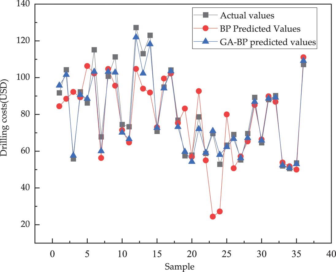
Figure 9: Comparison of predicted values of GA-BP and BP model test data

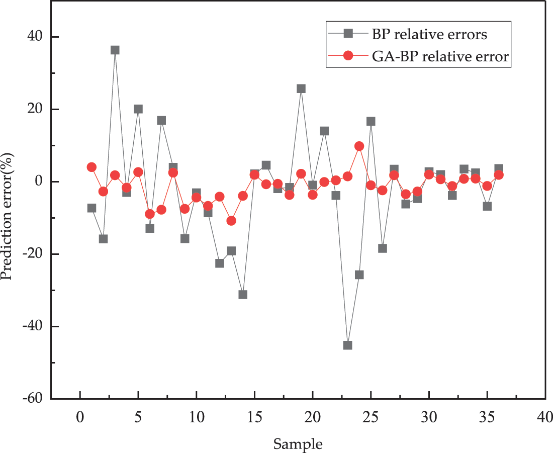
Figure 10: GA-BP and BP model test data prediction error comparison

After the optimization of GA algorithm, the neural network prediction model has reduced all kinds of computational indexes compared with the traditional BP model, which are shown in Table 4. As shown in Table 4, RMSE decreased by 25.38 (from 31.64 to 6.26), MAE decreased by 12.12 (from 17.88 to 5.76), MAPE decreased by 18.30% (from 21.56% to 3.26%). According to the above analysis, it is easy to tell that the GA algorithm improve the model’s capacity on a certain degree, and the GA-BP drilling costs hybrid model is much better than the traditional BP neural network model.

5  Conclusion

Cost is an important parameter of an investment project. Overestimating or underestimating the cost of drilling can lead to high risks in the financial and production management of the project. The current paper analyzed the dominant factors of drilling costs and selected relative features as the input model. Those inputs combined with the output, drilling costs, are applied for BP model training and testing. Furtherly, GA is introduced for initial weights and bias tuning. The hybrid model predicted the drilling costs of deep wells with ultra-deep wells, and finally research results with the base model are compared and evaluated.

The following main conclusions were drawn:

(1) The GA optimized drilling costs prediction model can obtain the optimal weights and bias quickly, the probability of falling into the local optimum phenomenon is also reduced. The reduction in RMSE is 25.38.

(2) The GA-BP model is a robust model for predicting drilling costs with an average error of less than 4%. Based on the proposed GA-BP model, the prediction model is well trained, and the prediction accuracy meets the requirements of cost estimation.

(3) The study demonstrates the feasibility and effectiveness of data-driven models for drilling costs forecasting applications, and the sample data can further improve the accuracy of the prediction models.

Funding Statement: This publication is based on work supported by the Science and Technology Innovation Foundation of CNPC “Multiscale Flow Law and Flow Field Coupling Study of Tight Sandstone Gas Reservoir” (2016D-5007-0208), and 13th Five-Year National Major Project “Multistage Fracturing Effect and Production of Fuling Shale Gas Horizontal Well Law Analysis Research” (2016ZX05060-009).

Author Contributions: Wenhua Xu: Conceptualization, Software, Writing-Original Draft, Writing-Review & Editing; Yingrong Wei: Conceptualization, Methodology; Yuming Zhu: Validation, Software, Validation; Dehua Liu: Methodology, Supervision; Hui Ji: Software; Ya Su: Resources.

Conflicts of Interest: The authors declare that they have no conflicts of interest to report regarding the present study.

References

1. Wang, H., Ge, Y., Shi, L. (2017). Current status, challenges and development direction of ultra-deep well drilling and completion technology in the 13th Five-Year Plan. Natural Gas Industry, 37(4), 1–8. [Google Scholar]

2. Lei, Q., Yun, X., Yang, Z., Cai, B., Li, S. (2021). Progress and development directions of stimulation techniques for ultra-deep oil and gas reservoirs. Petroleum Exploration and Development, 48(1), 221–231. https://doi.org/10.1016/S1876-3804(21)60018-6 [Google Scholar] [CrossRef]

3. Yuan, J., Luo, D., Feng, L. (2015). A review of the technical and economic evaluation techniques for shale gas development. Applied Energy, 148(1), 49–65. https://doi.org/10.1016/j.apenergy.2015.03.040 [Google Scholar] [CrossRef]

4. Lukawski, M. Z., Silverman, R. L., Tester, J. W. (2016). Uncertainty analysis of geothermal well drilling and completion costs. Geothermics, 64, 382–391. https://doi.org/10.1016/j.geothermics.2016.06.017 [Google Scholar] [CrossRef]

5. Kaiser, M. J., Pulsipher, A. G. (2007). Generalized functional models for drilling cost estimation. SPE Drilling & Completion, 22(2), 67–73. https://doi.org/10.2118/98401-PA [Google Scholar] [CrossRef]

6. Kitchel, B. G., Moore, S. O., Banks, W. H., Borland, B. M. (1997). Probabilistic drilling-cost estimating. SPE Computer Applications, 9(4), 121–125. https://doi.org/10.2118/35990-PA [Google Scholar] [CrossRef]

7. Shilling, R. B., Lowe, D. E. (1990). Systems for automated drilling AFE cost estimating and tracking. Petroleum Computer Conference, Denver, Colorado. [Google Scholar]

8. Rodriguez, R. U. (2015). A simple yet effective approach to estimate time and costs for the drilling project in the tapir field. SPE Latin American and Caribbean Petroleum Engineering Conference, Quito, Ecuador. [Google Scholar]

9. Akins, W. M., Abell, M. P., Diggins, E. M. (2005). Enhancing drilling risk & performance management through the use of probabilistic time & cost estimating. Society of Petroleum Engineers, Amsterdam, Netherlands. [Google Scholar]

10. Ugochukwu, O. (2016). The use of risk analysis and probabilistic methods for more accurate time and cost estimates in subsea intervention operations. SPE Nigeria International Conference & Exhibition, Lagos, Nigeria. [Google Scholar]

11. Zhao, Y., Zhao, S. Z., Liu, T. S. (2011). Bayesian regularization BP neural network model for predicting oil-gas drilling costs. International Conference on Business Management & Electronic Information, Guangzhou, Guangdong, China, IEEE. [Google Scholar]

12. Guo, H., Nguyen, H., Vu, D. A., Bui, X. N. (2021). Forecasting mining capital cost for open-pit mining projects based on artificial neural network approach. Resources Policy, 74(3), 101474. https://doi.org/10.1016/j.resourpol.2019.101474 [Google Scholar] [CrossRef]

13. Zheng, X., Nguyen, H., Bui, X. N. (2021). Exploring the relation between production factors, ore grades, and life of mine for forecasting mining capital cost through a novel cascade forward neural network-based salp swarm optimization model. Resources Policy, 74, 102300. https://doi.org/10.1016/j.resourpol.2021.102300 [Google Scholar] [CrossRef]

14. Li, G., Wu, B., Hou, J., Wang, H., Wang, J. et al. (2022). Mining cost prediction model for underground metal mines. Metal Mining, 5, 62–69. [Google Scholar]

15. Wang, S., Zhang, N., Wu, L., Wang, Y. (2016). Wind speed forecasting based on the hybrid ensemble empirical mode decomposition and GA-BP neural network method. Renewable Energy, 94, 629–636. https://doi.org/10.1016/j.renene.2016.03.103 [Google Scholar] [CrossRef]

16. Si, S., Sun, X. (2011). Mathematical modeling algorithms and applications. Beijing, China: National Defense Industry Press. [Google Scholar]

17. Li, X., Guo, Z., Hu, Y., Liu, X., Wan, Y. et al. (2020). Challenges, countermeasures and suggestions for high-quality development of ultra-deep and large gas fields in China. Natural Gas Industry, 40(2), 75–82. [Google Scholar]

18. Kaiser, M. J., Yu, Y. (2015). Drilling and completion cost in the Louisiana Haynesville Shale, 2007–2012. Natural Resources Research, 24(1), 5–31. https://doi.org/10.1007/s11053-014-9229-9 [Google Scholar] [CrossRef]

19. Si, G., Wei, L., Huang, W., Guo, Z., Chen, Y. (2009). The main factors affecting drilling costs and control measures. Natural Gas Industry, 29(9), 106–109. [Google Scholar]

20. Guan, D., Luo, Y., Zhang, X. D., Guo, S. (2012). Research on the analysis and prediction method of the influencing factors of offshore drilling costs. Drilling Technology, 35(4), 41–43. [Google Scholar]